Lens aberrations and diffraction are two basic factors that limit lens sharpness. Details regarding these basis factors are provided in the following sections.
Lens Aberrations
Imperfections in optical systems arise from a number of causes that include different bending of light at different wavelengths, the inability of spherical surfaces to provide clear images over large fields of view, changes in focus for light rays that don’t pass through the center of the lens, and many more (i.e., coma, stigmatism, spherical aberration, and chromatic aberration). Aberration correction is the primary purpose of sophisticated lens design and manufacturing, and it is what distinguishes an excellent from a mediocre optical design.
Lens aberrations worsen at large apertures (small f-numbers) and vary greatly for different lenses, even among different samples of the same lens; i.e., the quality control of mass-produced lenses does not always produce lenses of identical quality
Diffraction
Diffraction is a fundamental physical property that blurs images. It is caused by the bending of light waves near boundaries. The smaller the aperture (the larger the f-number), the worse the diffraction blur. Since diffraction is a fundamental physical effect, diffraction is the same for all lenses. Lens performance does not vary significantly at small apertures (large f-numbers). In other words, the lens’ f-stop number is equal to its focal length divided by its aperture diameter. In the classic f-stop sequence
{ 1 1.4 2 2.8 4 5.6 8 11 16 22 32 45 64 …}
each stop admits half the light of the previous stop, while the f-stop number is multiplied by the square root of 2 (1.414). When a photographer says, “I increased the exposure by one f-stop,” then the sequence is decreased by one step; e.g., the aperture changes from f/8 to f/5.6.
As a result, lenses tend to have an optimum aperture where they are sharpest, typically around 2 to 3 f-stops below a lens’ maximum aperture. The optimum is fairly broad because the aperture can usually be off by up to two f-stops away without serious sharpness loss.
You can find the optimum aperture by running a batch of images (Imatest SFRplus or eSFR ISO recommended) taken at different apertures, then entering the combined output (a CSV file) into Batchview (Figure 1).
Figure 1. Set of images taken at f/4.5 to f/22
In Figure 1, bars show MTF50 in line widths per picture height (LW/PH) for the weighted mean (black), center area (red), part-way area (green), and corners (blue). The procedure is described in detail here. For the lens results in Figure 1, the optimum aperture is 2 to 3 stops from the maximum and edge sharpness is unimpressive.
In Figure 2, diffraction-limited MTF is displayed as a pale brown dotted curve in the MTF figures produced by SFR, SFRplus, and eSFR ISO when the pixel spacing (usually in microns) has been manually entered in the appropriate dialog box.
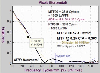
Figure 2. MTF plots showing diffraction-limited MTF (as a pale brown dotted line)
In this figure, the curve on the left is for the Canon EOS-40D (5.7-micron pixel spacing) with the lens set at f/22, which is a small aperture that should only be used when large depth of field is required and sharpness can be sacrificed.
The equation for diffraction-limited MTF can be found in Diffraction Modulation Transfer Function from the SPIE OPTIPEDIA, David Jacobson’s Lens Tutorial, and normankoren.com. The diffraction cutoff frequency is
\(\displaystyle f_{\mathit{cutoff}} = \frac{1}{\lambda N}\)
where λ is the wavelength and N is the f-stop number. λ is typically 0.555 microns (0.000555mm) for visible light, but it can be changed for cameras with different spectral response (like Infrared).
Let
\(\displaystyle s=\frac{f}{f_{\mathit{
The diffraction-limited MTF is
\(\mathit{MTF}_{\mathit{
\(\mathit{MTF}_{\mathit{
Figure 2 is also shown with a Data Cursor Datatip, which allows you to examine plot or image pixel values.
Lens MTF response can never exceed the diffraction-limited response, but system MTF response often exceeds it at medium spatial frequencies as a result of sharpening, which is (and should be) present in most digital imaging systems.
In addition to lens response, system MTF response is affected by the sensor (which has a null at 1 cycle/pixel = 2×Nyquist frequency), the anti-aliasing filter (designed to suppress energy above 0.5 cycles/pixel), and signal processing (which can be very complex and can be different in different regions of an image).