Introduction – MTF – MTF equation – Slanted-edge measurements – Why a slanted edge? – MTF measurement matrix
Spatial frequency units – Summary metrics – Results – Noise reduction – Diffraction & Optimum aperture
Interpreting MTF50 – Auto-focus – Calculation details – Imatest vs. ISO calculation – Links
Introduction
Sharpness is arguably the most important photographic image quality factor because it determines the amount of detail an imaging system can reproduce. Imatest also measures a great many others.
Sharpness is defined by the boundaries between zones of different tones or colors. It is illustrated by the bar pattern of increasing spatial frequency, below. The top portion is sharp; its boundaries are crisp steps, not gradual. The bottom portion illustrates how the pattern is degraded after it passes through a lens. It is blurred. All lenses, even the finest, blur images to some degree. Poor lenses blur images more than fine ones.

Bar pattern: Original (top); with lens degradation (bottom)
One way to measure sharpness is to use the rise distance of the edge, for example, the distance (in pixels, millimeters, or fraction of image height) for the pixel level to go from 10% to 90% of its final value. This is called the 10-90% rise distance. Although rise distance is a good indicator of image sharpness, it has an important limitation. There is no simple way to calculate the rise distance of a complete imaging system from the rise distance of its components— from a lens, digital sensor, and software sharpening.
To get around this problem, measurements are made in frequency domain, where frequency is measured in cycles or line pairs per distance (millimeters, inches, pixels, image height, and sometimes angle (degrees or milliradians)). Line pairs per millimeter (lp/mm) was the most common spatial frequency unit for film, but cycles/pixel (C/P) and line widths/picture height (LW/PH) are more convenient for digital sensors.
The image below is a sine wave— a pattern of pure tones— that varies from low to high spatial frequencies. The top portion is the original sine pattern. The bottom portion illustrates lens degradation, which reduces pattern contrast at high spatial frequencies.

Sine pattern: Original (top); with lens degradation (bottom)
The relative contrast at a given spatial frequency (output contrast/input contrast) is called the Modulation Transfer Function (MTF) or Spatial Frequency Response (SFR). It is the key to measuring sharpness.
Modulation Transfer Function (MTF)
Modulation Transfer Function (MTF), which is generally identical to Spatial Frequency Response (SFR), can be explained using the illustration below.
Sine and bar patterns, amplitude plot, and Contrast (MTF) plot
The upper plot displays
- the original sine pattern
- the sine pattern with lens blur
- the original bar pattern
- the bar pattern with lens blur
Lens blur causes contrast to drop at high spatial frequencies.
The middle plot displays the luminance (“modulation”; V in the equation below) of the bar pattern with lens blur (the red curve). Contrast decreases at high spatial frequencies. The modulation of the sine pattern (which consists of pure frequencies) is used to calculate MTF.
The lower plot displays the corresponding sine pattern contrast, i.e., MTF (SFR) (the blue curve), which is defined below.
By definition, the low frequency MTF limit is always 1 (100%). For this (virtual) lens, MTF is 50% at 61 lp/mm and 10% at 183 lp/mm.
Both frequency and MTF are displayed on logarithmic scales with exponential notation (100 = 1; 101 = 10; 102 = 100, etc.). Amplitude is displayed on a linear scale.
The beauty of using MTF (Spatial Frequency Response) is that the MTF of a complete imaging system is the product of the MTF of its individual components.
The equation for MTF is derived from the sine pattern contrast C(f) at spatial frequency f, where
\(\displaystyle C(f) = \frac{V_{max} – V_{min}}{V_{max} + V_{min}}\) for luminance (“modulation”) V.
\(MTF(f) = 100% \times C(f) / C(0)\) This normalizes MTF to 100% at low spatial frequencies
To normalize MTF at low spatial frequencies, test chart must have a low frequency reference. This is satisfied by the large light and dark areas in slanted-edges and also by features in most of the other patterns used by Imatest, but it is not satisfied by lines and grids, which is why there aren’t used for Imatest MTF analysis.
Were you passionate about your college math classes?
Then you’re probably a math geek— a member of a misunderstood but highly elite fellowship. The text in green is for you. If you’re a normal person or mathematically challenged, you may skip these sections. You’ll never know what you missed.
The primary Imatest MTF calculation is the slanted-edge, which uses a mathematical operation known as the Fourier transform. MTF is the Fourier transform of the impulse response— the response to a narrow line, which is the derivative (d/dx or d/dy) of the edge response. Fortunately, you don’t need to understand Fourier transforms or calculus to understand MTF.
-
USAF 1951 chart. Not supported by Imatest.
Traditional “resolution” measurements involve observing an image of a bar pattern (often the USAF 1951 chart), and looking for the highest spatial frequency (in lp/mm) where the bars are visibly distinct. This measurement, also called “vanishing resolution”, corresponds to an MTF of roughly 10-20%. Because this is the spatial frequency where image information disappears— where it isn’t visible, it’s strongly dependent on observer bias, and hence it’s a poor indicator of image sharpness. (It’s Where the Woozle Wasn’t in the world of Winnie the Pooh.) The USAF chart is also poorly suited for computer analysis because it uses space inefficiently and the bar triplets lack a low frequency reference.
Experience has shown that the best indicators of image sharpness are the spatial frequencies where MTF is 50% of its low frequency value (MTF50) or 50% of its peak value (MTF50P).
MTF50 or MTF50P are good parameters for comparing the sharpness of different cameras and lenses for two reasons: (1) Image contrast is half its low frequency or peak values,hence detail is still quite visible. The eye is relatively insensitive to detail at spatial frequencies where MTF is low: 10% or less. (2) The response of most cameras falls off rapidly in the vicinity of MTF50 and MTF50P. MTF50P is a better metric for strongly sharpened cameras that have “halos” near edges and corresponding peaks in their MTF response.
Although MTF can be estimated directly from images of sine patterns (using Rescharts Log Frequency, Log F-Contrast, and Star Chart), a sophisticated technique, based on the ISO 12233 standard, “Photography – Electronic still picture cameras- Resolution measurements,” provides more accurate and repeatable results and uses space far more efficiently. (See Slanted-edge versus Siemens Star for more detail.) A slanted-edge image, described below, can be photographed, then analyzed by Imatest SFR, SFRplus, or eSFR ISO.
| Origins of Imatest slanted-edge SFR calculations: The algorithms were adapted from a Matlab program, sfrmat, written by Peter Burns ( |
The slanted-edge measurement for Spatial Frequency Response
Several Imatest modules, listed below, measure MTF using the slanted-edge technique.
Slanted-edge test charts may be purchased from Imatest or created with Imatest Test Charts. Charts that employ automatic detection (SFRplus, eSFR ISO, SFRreg, or Checkerboard) are recommended.
Briefly, the ISO 12233 slanted edge method calculates MTF by finding the average edge (4X oversampled using a clever binning algorithm), differentiating it (to obtain the Line Spread Function (LSF)), then taking the absolute value of the Fourier transform of the LSF. The algorithm is described in detail here.
| Why a slanted edge? MTF results for pure vertical or horizontal edges are highly dependent on sampling phase (the relationship between the edge and the pixel locations), and hence can vary from one run to the next depending on the precise (sub-pixel) edge position. The edge is slanted so MTF is calculated from the average many sampling phases, which makes results much more stable and robust. |
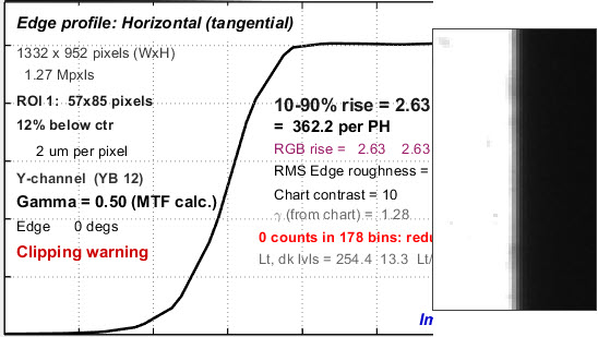 Clipped high-contrast vertical edge: Clipped high-contrast vertical edge:Results are NOT valid. |
| Edge contrast should be limited to 10:1 at the most. 4:1 edge contrast is generally recommended. The reason is that high contrast edges (>10:1, such as found in the old ISO 12233:2000 chart) can cause saturation or clipping, resulting in edges with sharp corners that exaggerate MTF measurements. |
The slanted-edge method has several advantages.
- The camera-to-target distance is not critical; it doesn’t enter into the equation that converts the image into MTF response (it is scale-invariant).
- Slanted-edges also take up much less space than sine patterns and are less sensitive to noise.
- MTF can be measured above the Nyquist frequency (0.5 cycles/pixel) thanks to the binning/oversampling algorithm.
Imatest Master can calculate MTF for edges of virtually any angle, though exact vertical, horizontal, and 45° should be avoided because of sampling phase sensitivity.
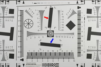
SFR measures MTF from slanted-edges in a wide variety of charts— wherever there is a clean edge. Region selection is manual. Two useful regions in the old ISO-12233:2000 chart (on the right; no longer an official part of the ISO standard) are indicated by the red and blue arrows. ISO 12233 charts have been used in imaging-resource.com and dpreview.com camera reviews. A typical region— a crop of a vertical edge (slanted about 5.7 degrees) used to calculate horizontal MTF response— is shown on the far right. |
 |
| The following charts have automatic region detection. | |
| SFRplus measures MTF and many other image quality parameters from the SFRplus chart, which can be purchased from Imatest (recommended) or created using Imatest Test Charts (a wide body printer, good printing skills, and knowledge of color management are required). It offers numerous advantages over the old ISO 12233:2000 test chart: automatic feature detection, lower contrast for improved accuracy, more edges (less wasted space) for a detailed map of MTF over the image surface. Measurements are ISO-compliant. |  |
| eSFR ISO also measures MTF and other image quality parameters using an enhanced version of the new ISO 12233:2014 Edge SFR (E-SFR) test chart. It has slightly less spatial detail than SFRplus, but much more noise detail. The old ISO 12233:2000 test chart (shown above) is no longer an official part of the ISO 12233 standard. | 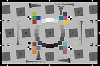 |
| Checkerboard is very insensitive to framing, making it ideal for through-focus tests, and it also has very precise distortion calculations. | 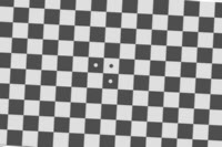 |
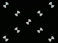
| SFRreg Several individual charts are typically placed around the image field. Works with – extreme fisheye lenses (>180º) – charts at different distances to test focus & depth of field. – extreme high resolution (>36MP) cameras, large Fields of View, and large distances. |
 |
How to test lenses with Imatest has a good summary of how to measure MTF using SFRplus or eSFR ISO.
MTF Measurement Matrix
Imatest has many ways of measuring MTF, each of which tends to give different results in consumer cameras because image processing depends on local scene content, which is rarely constant throughout an image. Sharpening (high frequency boost) tends to be maximum near contrasty features, while noise reduction (high frequency cut, which can obscure fine texture) tends to be maximum in their absence. For this reason MTF measurements can be very different with different test charts.
In principle, MTF measurements should be the same when no nonuniform or nonlinear image processing is applied, for example when the image is demosaiced with dcraw with no sharpening and noise reduction. But this never happens in practice because demosaicing, which is present in all cameras that use Color Filter Arrays (CFAs) involves some nonlinear processing. Noise, for example, is handled differently from edges.
| Measurement pattern |
Advantages / Disadvantages / Sensitivity | Primary use & comments |
| Slanted-edge (SFR SFRplus eSFRISO SFRreg Checkerboard) |
Most efficient use of space: makes it possible to create a detailed map of MTF response. Fast, automated region detection in SFRplus, eSFR ISO, SFRreg, and Checkerboard. Fast calculations. Relatively insensitive to noise (highly immune if noise reduction is applied). Compliant with the ISO 12233 standard, whose “binning” (super-resolution) algorithm allows MTF to be measured above the Nyquist frequency (0.5 C/P). The best pattern for manufacturing testing. May give optimistic results in systems with strong sharpening and noise reduction (i.e., it can be fooled by signal processing, especially with high contrast (≥ 10:1) edges. Gives inconsistent results in systems with extreme aliasing (strong energy above the Nyquist frequency), especially with small regions. Most sensitive to sharpening, especially for high contrast (≥10:1) edges; less sensitive for low contrast edges (≤2:1). Least sensitive to software noise reduction. |
This is the primary MTF measurement in Imatest. The most efficient pattern for lens and camera testing, especially where an MTF response map is required. The high contrast (≥40:1) recommended in the old ISO 12233:2000 standard produced unreliable results (clipping, gamma issues). The new ISO 12233:2014 standard recommends 4:1 contrast. This is our recommendation (with SFRplus or eSFR ISO) for all new work. Compared favorably with the Siemens star in Slanted-edge versus Siemens Star. |
| Log frequency | Calculated from first principles. Displays color moire. Sensitive to noise. Inefficient use of space. |
Primarily used as a check on other methods, which are not calculated from first principles. |
| Log f-Contrast | Sensitive to noise. Strong sensitivity to sharpening near the (high contrast) top of the image; strong sensitivity to noise reduction near the (low contrast) bottom, with a gradual transition in-between. |
>Illustrates how signal processing varies with image content (feature contrast). Shows loss of fine detail due to software noise reduction. |
| Siemens star | Included in the ISO 12233:2014 standard. Relatively insensitive to noise. Provides directional MTF information. Slow, inefficient use of space. Limited low frequency information at outer radius makes MTF normalization difficult. Moderate sensitivity to sharpening and noise reduction. |
Promoted for general testing by Image Engineering, but spatial detail is limited to a 3×3 or 4×3 grid. Compared with the slanted-edge in Slanted-edge versus Siemens Star. |
| Dead Leaves (Spilled Coins) |
Measures texture blur / sharpness / acutance. Pattern statistics are similar to typical images. Inefficient use of space. A tricky noise power subtraction algorithm* is required to reduce very high sensitivity to noise. Moderate sensitivity to sharpening and strong sensitivity to noise reduction make it usable for an overall texture sharpness metric that correlates well with subjective observations. |
Consists of stacked randomly-sized circles. Strong industry interest, particularly from the Camera Phone Image Quality (CPIQ) group.
Both Dead Leaves (Spilled Coins) and Random charts are analyzed with the Random (Dead Leaves) module. |
| Random (scale-invariant) | Reveals how well fine detail (texture) is rendered: system response to software noise reduction. Lest sensitive to sharpening, Most sensitive to Software noise reduction |
Measures a camera’s ability to render fine detail (texture), i.e., low contrast, high spatial frequency image content. *Noise power can be removed from the measurement in Imatest using the gray patches adjacent to the pattern. |
| Wedge | Makes use of wedge patterns on the ISO 12233 chart. MTF is not accurate around Nyquist and half-Nyquist frequencies (it’s very sensitive to sampling phase variations). Not suitable as a primary MTF measurement. Sensitive to sharpening. Sensitive to noise. Inefficient use of space. |
Measures “vanishing resolution” from CIPA DC-003: where lines start disappearing in wedge patterns, most commonly in the ISO 12233 chart, where three regions (including a square region for a low-frequency reference) are required to get a reasonable MTF measurement (which is less accurate than other methods due to sampling phase sensitivity). |
Spatial frequency units and summary metrics
Most readers will be familiar with temporal frequency. The frequency of a sound— measured in Cycles/Second or Hertz— is closely related to its perceived pitch. The frequencies of radio transmissions (measured in kilohertz, megahertz, and gigahertz) are also familiar. Spatial frequency is similar: it is measured in cycles (or line pairs) per distance instead of time. Spatial frequency response is closely analogous to temporal (e.g., audio) frequency response. The more extended the response, the more detail can be conveyed.
 Spatial frequency units should be selected based on the application, for example, is the measurement intended to determine how much detail a camera can reproduce or how well the pixels are utilized?
Spatial frequency units are selected in the
Settings or More settings windows of
SFR and Rescharts modules (SFRplus, eSFR ISO, Star, etc.).
Film camera lens tests used line pairs per millimeter (lp/mm). This worked well for comparing lenses because most 35mm film cameras have the same 24x36 mm picture size. But digital sensor sizes varies widely, from under 5 mm diagonal in camera phones to 43 mm diagonal for full-frame DSLRs— even larger for medium format backs. For this reason, Line widths per picture height (LW/PH) is recommended for measuring the total detail a camera can reproduce. LW/PH is equal to 2 * lp/mm * (picture height in mm).
Another useful spatial frequency unit is cycles per pixel(C/P), which gives an indication of how well individual pixels are utilized. There is no need to use actual distances (millimeters or inches) with digital cameras, although such measurements are available in Imatest SFR, SFRplus, eSFR ISO, and all Rescharts modules.
Summary Metrics
Several summary metrics are derived from MTF curves to characterize overall performance. These metrics are used in a number of displays, including secondary readouts in the SFR/SFRplus/eSFR ISO Edge/MTF plot (shown below) and in the SFRplus 3D maps.
| Summary metric | Description | Comments |
| MTF50 MTFnn |
Spatial frequency where MTF is 50% (nn%) of the low (0) frequency MTF. MTF50 (nn = 50) is widely used because it corresponds to bandwidth (the half-power frequency) in electrical engineering. | The most common summary metric; correlates well with perceived sharpness. Increases with increasing software sharpening; may be misleading because it “rewards” excessive sharpening, which results in visible and possibly annoying “halos” at edges. |
| MTF50P MTFnnP |
Spatial frequency where MTF is 50% (nn%) of the peak MTF. | Identical to MTF50 for low to moderate software sharpening, but lower than MTF50 when there is a software sharpening peak (maximum MTF > 1). All in all, a better metric then MTF50. |
| MTF area normalized |
Area under an MTF curve (below the Nyquist frequency), normalized to its peak value (1 at f = 0 when there is little or no sharpening, but the peak may be » 1 for strong sharpening). | A particularly interesting new metric because it closely tracks MTF50 for little or no sharpening, but does not increase for strong oversharpening, i.e., it does not reward excessive sharpening. Still relatively unfamiliar. Described in Slanted-Edge MTF measurement consistency. |
| MTF10, MTF10P, MTF20, MTF20P |
Spatial frequencies where MTF is 10 or 20% of the zero frequency or peak MTF | These numbers are sometimes used because they are comparable to the “vanishing resolution” (Rayleigh limit). Noise can strongly affect results at the 10% levels or lower. MTF20 in Line Widths per Picture Height (LW/PH) is closest to analog TV Lines. |
Imatest slanted-edge results
The Edge/MTF plot from Imatest SFR is shown below. SFRplus, eSFR ISO, SFRreg, and Checkerboard produce similar results and much more.
Edge/SFR results for an SFRplus image from a 10 Megapixel DSLR
(Upper-left) A narrow image that illustrates the tones of the averaged edge. It is aligned with the average edge profile (spatial domain) plot,immediately below.
(Middle-left) Average Edge (Spatial domain): The average edge profile shown here linearized, i.e., proportional to light energy. A key result is the edge rise distance (10-90%), shown in pixels and in the number of rise distances per Picture Height. Other parameters include overshoot and undershoot (if applicable). This plot can optionally display the line spread function (LSF: the derivative of the edge).
(Bottom-left) MTF (Frequency domain): The Spatial Frequency Response (MTF), shown to twice the Nyquist frequency. A key summary result is MTF50, the frequency where contrast falls to 50% of its low frequency value, which corresponds well with perceived image sharpness. It is given in units of cycles per pixel (C/P) and Line Widths per Picture Height (LW/PH). Other results include MTF at Nyquist (0.5 cycles/pixel; sampling rate/2), which indicates the probable severity of aliasing and user-selected secondary readouts. The Nyquist frequency is displayed as a vertical blue line. The diffraction-limited MTF response is shown as a pale brown dashed line when the pixel spacing is entered (manually) and the lens focal length is entered (usually from EXIF data, but can be manually entered).
For this camera, which is moderately sharpened, MTF50P (displayed only when the Standardized sharpening display is unchecked) is identical to MTF50.
Click on the thumbnails or image below so see the relationship between visible sharpness and Edge and MTF measurements for the Canon EF 17-85mm zoom at 26mm, f/5.6, which is not a great lens— sharpness falls off badly in the corners— but makes an excellent example. The first image shows a 3D map of MTF50 over the image surface. The remaining images show the enlarged edge and the edge profile and MTF measurements for several regions. To obtain this plot, Run an SFRplus or eSFR ISO image in Rescharts (you can click ), then Select 8. Image & Geometry with the Crop to ROI option (or you check a box in the Edge and MTF plot). After you click on the region (1. Center V, etc.) you can quickly scroll through regions using your keyboard’s up and down-arrows (↑ and ↓).
Note that at typical screen resolutions the edge shown above would be contained in an image around 1 meter high.
SFR Results: MTF (sharpness) plot describes this Figure in detail.
MTF curves and Image appearance contains several examples illustrating the correlation between MTF curves and perceived sharpness.
Noise reduction (modified apodization technique)
A powerful noise reduction technique called modified apodization is available for slanted-edge measurements (SFR, SFRplus, eSFR ISO, SFRreg, and Checkerboard). This technique makes virtually no difference in low-noise images, but it can improve measurement consistency for noisy images, especially at high spatial frequencies (f > Nyquist/2). It is applied when the MTF noise reduction (modified apodization) checkbox is checked in settings windows for any of the slanted-edge modules or in the Rescharts More settings window. ISO standard SFR (lower-left of the window) must be unchecked.
Note that we recommend keeping it enabled even though it is NOT a part of the ISO 12233 standard. If the ISO standard checkbox is checked (at the bottom-left of the dialog boxes), noise reduction is not applied.
The strange word apodization* comes from “Comparison of Fourier transform methods for calculating MTF” by Joseph D. LaVeigne, Stephen D. Burks, and Brian Nehring, available on the Santa Barbara Infrared website. The fundamental assumption is that all important detail (at least for high spatial frequencies) is close to the edge. The original technique involves setting the Line Spread Function (LSF) to zero beyond a specified distance from the edge. The modified technique strongly smooths (lowpass filters) the LSF instead. This has much less effect on low frequency response than the original technique, and allows tighter boundaries to be set for better noise reduction.
*Pedicure might be a better name for this technique, but it might confuse the uninitiated.
Modified apodization: original noisy averaged Line Spread Function (bottom; green),
smoothed (middle; blue), LSF used for MTF (top; red)
Algorithm
- The LSF (derivative of the average edge response; the green curve at the bottom of the above figure) is smoothed (lowpass filtered) to create the blue curve in the middle. Smoothing is accomplished by taking the 9 point moving average (the average of 9 adjacent points). Note that these samples are 4x oversampled as a result of the binning algorithm, so they correspond to approximately 2 samples in the original image. The smoothing eliminates most response above the Nyquist frequency (0.5 cycles/pixel).
- The boundaries where the values of the smoothed curve are greater than 20% of the peak value {BL, BU} are located. \(PW20 = B_U – B_L\) is the difference between these boundaries.
- The apodization boundaries are located at \(A_L = B_L – PW20 – 4\) and \(A_U = B_U + PW20 + 4\) (pixels). This allows for sufficient “breathing room” so important detail near the edge is unaffected.
- The LSF used for calculating MTF is set to the original (unsmoothed) LSF inside the apodization boundaries {AL, AU} and to the smoothed LSF outside.
The benefits of modified apodization noise reduction are shown below for an image with strong (simulated) white noise.
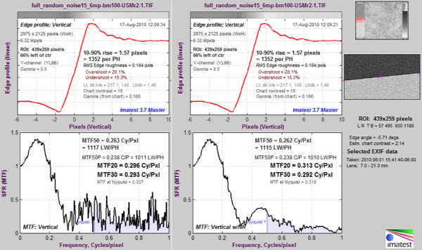
Modified apodization noise reduction on a noisy image: without (L) and with (R)
Diffraction and Optimum Aperture
Lens sharpness is limited by two basic factors.
- Lens Aberrations Imperfections in optical systems that arise from a number of causes— different bending of light at different wavelengths, the inability of spherical surfaces to provide clear images over large fields of view, changes in focus for light rays that don’t pass through the center of the lens, and many more. Aberration correction is the primary purpose of sophisticated lens design and manufacturing; It’s what distinguishes excellent from mediocre optical design.
Lens aberrations tend to be worst at large apertures (small f-numbers). Aberrations vary greatly for different lenses (and even among of different samples of the same lens); quality control mass-produced lenses is often quite sloppy.
- Diffraction A fundamental physical property that blurs images. Diffraction is caused by the bending of light waves near boundaries.The smaller the aperture (the larger the f-number), the worse the diffraction blur. Since it’s a fundamental physical effect, it’s the same for all lenses. Lens performance doesn’t vary a lot at small apertures (large f-numbers).
If you’re not familiar with this terminology, a lens’s f-stop number is equal to its focal length divided by its aperture diameter. In the classic f-stop sequence {1 1.4 2 2.8 4 5.6 8 11 16 22 32 45 64…}, each stop admits half the light of the previous stop while the f-stop number is multiplied by the square root of 2 (1.414). When a photographer says, “I increased the exposure by one f-stop”, he means he went down the sequence by one step, e.g., changed the aperture from f/8 to f/5.6.
Batchview result
As a result of these two phenomena, lenses tend to have an optimum aperture where they are sharpest, typically around 2-3 f-stops below a lens’s maximum aperture. The optimum is fairly broad: the aperture can usually be off by up to two f-stops away without serious sharpness loss.
You can find the optimum aperture by running a batch of images (Imatest SFRplus or eSFR ISO recommended) taken at different apertures, then entering the combined output (a CSV file) into Batchview. A set of images taken at f/4.5-f/22 is shown on the right: The bars show MTF50 in Line Widths per Picture Height (LW/PH) for the weighted mean (black), center area (red), part-way area (green) and corners (blue). The procedure is described in detail here. For this lens the optimum aperture is 2-3 stops from the maximum. Edge sharpness is unimpressive. It’s not one of Canon’s better efforts.
 MTF plots showing diffraction-limited MTF (as a pale brown dotted line) |
Diffraction-limited MTF is displayed as a pale brown dotted curve in the MTF figures produced by SFR, SFRplus, and eSFR ISO when the pixel spacing (usually in microns) has been manually entered in the appropriate input dialog box. The curve on the left is for the Canon EOS-40D (5.7 micron pixel spacing) with the lens set at f/22— a small aperture that should only be used with large depth of field is required and sharpness can be sacrificed. The equation for diffraction-limited MTF can be found in Diffraction Modulation Transfer Function from the SPIE OPTIPEDIA, David Jacobson’s Lens Tutorial, and normankoren.com. The diffraction cutoff frequency is \(f_{cutoff} = frac{1}{lambda N}\) where λ is the wavelength and N is the f-stop number. λ is typically 0.555 microns (0.000555 mm) for visible light, but it can be changed for cameras with different spectral response (like Infrared). |
Let \( s = f / f_{cutoff}\). The diffraction-limited MTF is
\(MTF_{diffraction-ltd}(s) = frac{2}{pi} bigl(arccos(s) – s sqrt{1-s^2}bigr)\) for s < 1
= 0 for s >= 1
The figure is shown with a Data Cursor Datatip, which allows you to examine plot or image pixel values. It is available in all figures and interactive GUIs in Imatest 3.6+.
Lens MTF response can never exceed the diffraction limited response, but system MTF response often exceeds it at medium spatial frequencies as a result of sharpening, which is (and should be) present in most digital imaging systems.
In addition to lens response, system MTF response is affected by the sensor (which has a null at 1 cycle/pixel), the anti-aliasing filter (designed to suppress energy above 0.5 cycles/pixel), and signal processing (which can be very complex— it can be different in different regions of an image).
Interpreting MTF50
This section was written before the addition of SQF (Subjective Quality Factor) to Imatest (November 2006). SQF allows a more refined estimate of perceived print sharpness.
What MTF50 do you need? It depends on print size. If you plan to print gigantic posters (20×30 inches or over), the more the merrier. Any high quality 4+ megapixel digital camera (one that produces good test results; MTF50(corr) > 0.3 cycles/pixel) is capable of producing excellent 8.5×11 inch (letter-size; A4) prints. At that size a fine DSLR wouldn’t offer a large advantage in MTF. With fine lenses and careful technique (a different RAW converter from Canon’s and a little extra sharpening), my 6.3 megapixel Canon EOS-10D (corrected MTF50 = 1340 LW/PH) makes very good 12×18 inch prints (excellent if you don’t view them too closely). Prints are sharp from normal viewing distances, but pixels are visible under a magnifier or loupe; the prints are not as sharp as the Epson 2200 printer is capable of producing. Softness or pixellation would be visible on 16×24 inch enlargements. The EOS-20D has a slight edge at 12>x18 inches; it’s about as sharp as I could ask for. There’s little reason go go to a 12+ megapixel camera lie the EOS 5D, unless you plan to print larger. Sharpness comparisons contains tables, derived from images downloaded from two well-known websites, that compare a number of digital cameras. Several outperform the 10D.
The table below is an approximate guide to quality requirements. The equation for the left column is
| MTF50(Line Widths ⁄ inch on the print) = |
MTF50(LW ⁄ PH) |
| MTF50 in Line Widths ⁄ inch on the print |
Quality level— after post-processing, which may include some additional sharpening |
| 150 | Excellent— Extremely sharp at any viewing distance. About as sharp as most inkjet printers can print. |
| 110 | Very good— Large prints (A3 or 13×19 inch) look excellent, though they won’t look perfect under a magnifier. Small prints still look very good. |
| 80 | Good— Large prints look OK when viewed from normal distances, but somewhat soft when examined closely. Small prints look soft— adequate, perhaps, for the “average” consumer, but definitely not “crisp.” |
Example of using the table: My Canon EOS-10D has MTF50 = 1335 LW/PH (corrected; with standardized sharpening). When I make a 12.3 inch high print on 13×19 inch paper, MTF50 is 1335/12.3 = 108 LW/in: “very good” quality; fine for a print that size. Prints look excellent at normal viewing distances for a print this size.
This approach is more accurate than tables based on pixel count (PPI) alone (though less refined than SQF, below). Pixel count is scaled differently; the numbers are around double the MTF50 numbers. The EOS-10D has 2048/12.3 = 167 pixels per inch (PPI) at this magnification. This table should not be taken as gospel: it was first published in October 2004, bandit may be adjusted in the future.
Acutance and Subjective Quality Factor (SQF)
SQF as a function of picture height
MTF is a measure of device or system sharpness, and is only indirectly related to the perceived sharpness when a display or print is viewed. A more refined estimate of perceived sharpness must include assumptions about the display size, viewing distance (typically proportional to the square root of display or print height), and the human visual system (the human eye’s Contrast Sensitivity Function (CSF)). Such an formula, called Subjective Quality Factor (SQF) developed by Kodak scientists in 1972, is included in Imatest. It has been verified and used inside Kodak and Polaroid, but it has remained obscure until now because it was difficult to calculate. Its only significant public exposure has been in Popular Photography lens tests. Imatest can also calculate a closely-related measurement called Acutance, developed by the Camera Phone Image Quality (CPIQ) initiative, and defined in the CPIQ 2.0 Specification document. Write support at imatest dot com for more information.
A portion of the Imatest SFR SQF figure for the EOS-10D is shown on the right. SQF is plotted as a function of display size. Viewing distance (pale blue dashes, with scale on the right) is assumed to be proportional to the square root of picture height. SQF is shown with and without standardized sharpening. (They are very close, which is somewhat unusual.) SQF is extremely sensitive to sharpening, as you would expect since sharpening is applied to improve perceptual sharpness.
The table below compares SQF for the EOS-10D with the MTF50 from the table above.
| MTF50 in Line Widths ⁄ inch on the print |
Corresponding print height for the EOS-10D (MTF50 = 1335 LW/PH) | SQF at this print height | Quality level— after post-processing, which may include some additional sharpening. Overall impression from viewing images at normal distances as well as close up. |
| 150 | 8.9 inches = 22.6 cm | 93 | Excellent— Extremely sharp. |
| 110 | 12.1 inches = 30.8 cm | 90 | Very good. |
| 80 | 16.7 inches = 42.4 cm | 86 | Good— Very good at normal viewing distance for a print of this size, but visibly soft on close examination. |
An interpretation of SQF is give here. Generally, 90-100 is considered excellent, 80-90 is very good, 70-80 is good, and 60-70 is fair. These numbers (which may be changed as more data becomes available) are the result of “normal” observers viewing prints at normal distances (e.g.., 30-34 cm (12-13 inches) for 10 cm (4 inch) high prints). The judgments in the table above are a bit more stringent— the result of critical examination by a serious photographer. They correspond more closely to the “normal” interpretation of SQF when the viewing distance is proportional to the cube root of print height (SQF = 90, 86, and 80, respectively), i.e., prints are examined more closely than the standard square root assumption.
An SQF peak over about 105 may indicate oversharpening (strong halos near edges), which can degrade image quality. SQF measurements are more valid when oversharpening is removed, which is accomplished with standardized sharpening.
Some observations on sharpness
- Frequency and spatial domain plots convey similar information,but in a different form. A narrow edge in spatial domain corresponds to a broad spectrum in frequency domain (extended frequency response), and vice-versa.
- Sensor response above the Nyquist frequency is garbage. It can cause aliasing,visible as Moire patterns of low spatial frequency. In Bayer sensors (all sensors except Foveon) Moire patterns appear as color fringes. Moire in Foveon sensors is far less bothersome because it’s monochrome and because the effective Nyquist frequency of the Red and Blue channels is lower than for Bayer sensors.
- Since MTF is the product of the lens and sensor response, demosaicing algorithm, and sharpening, and since sharpening typically boosts MTF at the Nyquist frequency, the MTF at and above the Nyquist frequency is not an unambiguous indicator of aliasing problems. It may, however, be interpreted as a warning that there could be problems.
- Results are calculated for the R, G, B, and Luminance (Y) channels, (by default, \(Y = 0.3R + 0.59G + 0.11B\), but Y can be set to a more modern value (\(0.2125R+0.7154G+0.0721B\)) in the Options I window). The Y channel is normally displayed in the foreground, but any of the other channels can selected. All are included in the .CSV output file.
- Horizontal and vertical resolution can be different for CCD sensors, and should be measured separately. They’re nearly identical for CMOS sensors. Recall, horizontal resolution is measured with a vertical edge and vertical resolution is measured with a horizontal edge.
- Resolution is only one of many criteria that contributes to image quality.
The ideal response would have high MTF below the Nyquist frequency and low MTF at and above it.
Slanted edge algorithm (calculation details)
The MTF calculation is derived from ISO standard 12233. Some details are contained in Peter Burns’ SFRMAT 2.0 or 3.0 User’s Guide. The Imatest calculation contains a number of enhancements, listed below. The original ISO calculation is performed when the ISO standard SFR checkbox in the SFR input dialog box is checked. It is normally unchecked.
- The cropped image is linearized, i.e., the pixel levels are adjusted to remove the gamma encoding applied by the camera. (Gamma is adjustable with a default of 0.5).
- The edge locations for the Red, Green, Blue, and luminance channels (\(Y = 0.3R + 0.59G + 0.11B\) or \(0.2125R + 0.7154G + 0.0721B\)) are determined for each scan line (horizontal lines in the above image).
- A second order fit to the edge is calculated for each channel using polynomial regression. The second order fit removes the effects of lens distortion. In the above image, the equation would have the form \( x = a_0 + a_1 y + a_2 y^2\).
- Depending on the value of the fractional part fp = xi – int(xi ) of the second order fit at each scan line, the shifted edge is added to one of four bins (bin 1 if 0 ≤ fp < 0.25; bin 2 if 0.25 ≤ fp < 0.5; bin 3 if 0.5 ≤ fp < 0.75; bin 4 if 0.75 ≤ fp < 1. (Correction 11/22/05: the bin does not depend on the detected edge location.)
- The four bins are combined to calculate an averaged 4x oversampled edge. This allows analysis of spatial frequencies beyond the normal Nyquist frequency.
- The derivative (d/dx) of the averaged 4x oversampled edge is calculated. A windowing function is applied to force the derivative to zero at its limits.
- MTF is the absolute value of the Fourier transform (FFT) of the windowed derivative.
Differences between Imatest and ISO 12233 calculations
- The center of each scan line is calculated from the peak of the lowpass-filtered edge derivative. The ISO calculation uses a centroid, which is optimum in the absence of noise. But noise is always present to some degree, and the centroid is extremely sensitive to noise because noise at large distances from the edge has the same weight as the edge itself.
- Gamma (used to linearize the data) is entered as an input value or derived from known chart contrast. In ISO-standard implementations it is assumed to be 1 unless an OECF file is entered.
- Imatest assumes that the edge may have some (second-order) curvature due to optical distortion. The ISO-standard calculation assumes a straight line, which can result in degraded MTF measurements in the presence of optical distortion. We are working on adding this enhancement to a future revision of ISO 12233
- Imatest’s “modified apodization” noise reduction (on by default) results in more consistent measurements (no systematic difference). It is turned off when the ISO standard calculation is checked.
Additional details of the calculation can be found in the Peter Burns links (below).
Links
Slanted-Edge MTF for Digital Camera and Scanner Analysis by Peter D. Burns (2000) (alternate source). An excellent introduction to the ISO 12233 slanted-edge measurement. Closely related: Diagnostics for Digital Capture using MTF by Don Williams and Peter D. Burns (2001), Applying and Extending ISO/TC42 Digital Camera Resolution Standards to Mobile Imaging Products by Don Williams and Peter D. Burns (2007) (Contains an image of the low-contrast slanted-edge test chart proposed for the revised ISO 12233 standard.)
How to Read MTF Curves by H. H. Nasse of Carl Zeiss. Excellent, thorough introduction. 33 pages long; requires patience. Has a lot of detail on the MTF curves similar to the Lens-style MTF curve in SFRplus. Even more detail in Part II.
Understanding MTF from Luminous Landscape.com has a much shorter introduction.
Understanding image sharpness and MTF A multi-part series by the author of Imatest, mostly written prior to Imatest’s founding. Moderately technical.
Bob Atkins has an excellent introduction to MTF and SQF. SQF (subjective quality factor) is a measure of perceived print sharpness that incorporates the contrast sensitivity function (CSF) of the human eye. It will be added to Imatest Master in late October 2006.
Spatial FrequencyResponse of Color Image Sensors: Bayer Color Filters and Foveon X3 by Paul M. Hubel, John Liu and Rudolph J. Guttosch, Foveon, Inc., Santa Clara, California. Uses slanted edge testing.
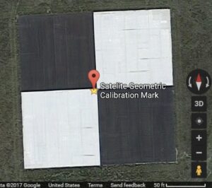
Calibration Targets (Google Earth Blog) Calibration targets– mostly for MTF– visible from satellites. Part 5. Around the world, is particularly interesting. A customer has used a target in 13300 Salon-de-Provence, France.