Introduction
Imatest’s slanted-edge algorithms for calculating MTF/SFR are based on ISO 12233 standard, “Photography – Electronic still picture cameras – Resolution measurements”. Although this standard is well-established in industry, we often receive questions regarding its validity. This document describes methods for validating the Imatest slanted-edge method for calculating image sharpness (expressed as Modulation Transfer Function, MTF, which is synonymous in practice with Spatial Frequency Response, SFR). MTF is a measurement of image contrast as a function of spatial frequency. As such, it is a measure of device or system sharpness, which is only indirectly related to perceived image sharpness in a print or display. SQF and Acutance measure perceived sharpness as a function of print or display height and viewing distance using formulas that include MTF, assumptions about viewing distance (often proportional to the square root of the print height, but other options are available) and the human visual system (the human eye’s Contrast Sensitivity Function.
Validating the Imatest slanted-edge method for calculating image sharpness
This document describes two validation strategies for the Imatest slanted-edge method for calculating image sharpness (MTF). The first strategy compares the Imatest slanted-edge method with SFRMAT3 (a MATLAB program). The second strategy compares the Imatest slanted-edge method with a first-principles (sine wave-based) calculation, which can be performed through ImageJ software.
Test Pattern:
To perform the validation we use a set of image files that contain patterns for both types of validation strategies. These files all start with the same image, but one is an unblurred original and the others are blurred to various degrees by an image editor program. The blurring is uniform throughout the image (unlike most consumer digital cameras, which have nonuniform processing: sharpening (high frequency boots) near edges; noise reduction (lowpass filtering) in their absence). Each image file contains several patterns.
- (Top) A bar pattern where spatial frequency varies with log(x). For reference only.
- (Middle) A sine pattern where spatial frequency varies with log(x). Generated with gamma = 1 (i.e., linear). This pattern is used to calculate MTF from first principles, as described below. It can be analyzed by the Imatest Log Frequency module or by ImageJ and Excel. The Log Frequency module is a part of Rescharts. To run it, click Modules, Rescharts in the Imatest main window.
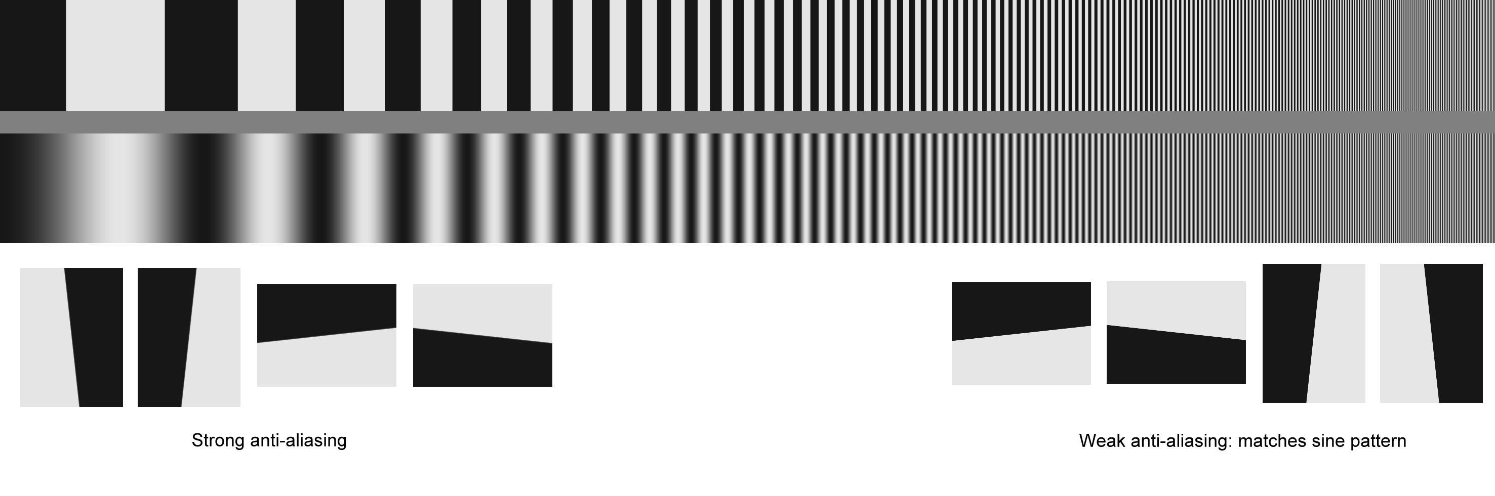 Original (unblurred) test pattern. Click to download full-sized image.
- (Lower-right) four slanted-edges that can be analyzed with Imatest SFR, Slanted-edge SFR (a part of Rescharts), or SFRMAT3. The anti-aliasing (AA) is similar to the AA used in generating the sine pattern. It’s fairly weak—some “stair-stepping” is visible on the edges. Contrast is also the same as the sine pattern (approximately 10:1).
The test patterns can be downloaded by clicking on the images on this page or from Slanted_edge_verification_patterns. In order of blurring, the file names are
- Logf_pattern_gamma1_contr10_2953W_3.png (the original; not blurred)
- Logf_pattern_gamma1_contr10_2953W_3-Blur.png
- Logf_pattern_gamma1_contr10_2953W_3-BlurMore.png
- Logf_pattern_gamma1_contr10_2953W_3-BlurGauss1.png
- Logf_pattern_gamma1_contr10_2953W_3-BlurGauss2.png
- Logf_pattern_gamma1_contr10_2953W_3-BlurGauss3.png (the most blurred)
Both the sine and slanted edges in the test pattern were created digitally. The bar and sine pattern at the top of the test image is initially created by the Imatest Test Charts module with the following settings: Pattern: Log Frequency-Contrast, PPI: 300, Highlight color: white, Type: bar, sine (4x), Frequency ratio: 200, Ink spread comp.: 0, Height: 20 cm, Contrast ratio: 10, Gamma: 1, Chart Lightness: Mid-light, Max frq cycles/width: 1000. The bar and sine pattern is a crop of the image produced by Test Charts.
A sharp, high-contrast edge can be created by a number of different approaches. A simple one is to run Imatest Test Charts, selecting SFR: quadrants, setting Contrast ratio to maximum and Gamma to 1, and then clicking Create test chart. The chart image is opened in an image editor, rotated approximately 5 degrees, and then cropped to fit in the final image (approximately 203×275 pixels for the above image). Since the rotation operation usually applies anti-aliasing that makes the slanted-edge less sharp than the sine pattern, the edge needs to be sharpened, with the amount determined by trial-and-error. The contrast is then reduced to about 10:1 (pixel levels between about 22 and 220) and versions of the image rotated by multiples of 90 degrees (which does not affect sharpness) are inserted into the final image. Details of the operations depend on the image editor selected.
Modulation Transfer Function (MTF)
The slanted-edge: a more convenient and reliable way of measuring MTF
MTF(f) is derived from slanted-edges by an abstract mathematical process, which is described in the ISO 12233 standard. Though abstract (not as direct as sine pattern measurements), it has several concrete advantages over sine patterns: it requires less real estate, it is more immune to noise, and it is very robust and repeatable. Essentially, MTF is the Fourier transform of the line spread function, which is the derivative of the average edge. Several edges are “binned” and averaged in a sophisticated process described in the ISO standard. The slant makes the measurement insensitive to sampling phase (edge location relative to pixel locations). The slanted-edge is compared with other MTF calculation methods here. The SPIE (the international society for optics and photonics) definition of MTF is in http://spie.org/x34298.xml
The sine pattern: for calculating MTF from first principals
For a sine pattern, modulation M is defined as \( M = \frac{A_{max} – A_{min}}{A_{max} + A_{min}}\) where Amax and Amin are the maximum and minimum values (amplitudes) of the sine pattern (the “envelope”). \( MTF(f) = M(f) / M(0)\), where f is spatial frequency and M(0) is the limiting value of M at low spatial frequencies. MTF(f) approaches 1 at f = 0, by definition. It may be larger than 1 for some frequencies, f > 0, in systems with software sharpening. MTF(f) can be thought of as the contrast of a sine pattern at spatial frequency f relative to low spatial frequencies. The spatial frequency where MTF drops by half, MTF50 (for 50%), is a good indicator of image sharpness, comparable to bandwidth in communication systems. We use it in the validation. MTF(f) is measured directly from the sine pattern in the chart using the Imatest Log Frequency module or, for independent verification, by ImageJ, which is described on http://normankoren.com/Tutorials/MTF5.html#ImageJ (an old web page predating Imatest), and can be downloaded from http://rsbweb.nih.gov/ij/. The Imatest Log-Frequency module calculates MTF(f) by detecting the envelope. The sophisticated algorithm works well at spatial frequencies approaching the Nyquist frequency (0.5 cycles/pixel; the highest meaningful frequency in digital systems).
Validation of Imatest MTF using SFRMAT3
In this validation Strategy, Imatest MTF values are compared with MTF values from SFRMAT3 using the same set of images. SFRMAT3 is a well-accepted implementation of the ISO 12233 standard that runs on MATLAB, and suitable for verifying the accuracy of Imatest calculations. SFRMAT3 was written by Peter Burns, who was a member of the ISO 12233 committee. At the time he was employed at Kodak along with Don Williams, with whom he has co-authored several papers on the slanted-edge method.
Installation and Requirements for SFRMAT3
SFRMAT3 is a Matlab program. The source code can be downloaded from Peter Burns’ web site.
Procedure to calculate MTF from SFRMAT3
- Open MATLAB.
- Open sfrmat3.m file into the MATLAB from the extracted zip folder.
- Run sfrmat3.m file and when asked load the input image to be verified using Imatest.
- The “Data Sampling & weights” window will appear. Nothing needs to be changed here. Click OK.
- The image file should be cropped by dragging the mouse—as in Imatest (but there is no fine adjustment). For agreement with Imatest, gamma = 1 files should be used (and Imatest should set for gamma = 1).
- The SFR vs. Frequency (cycle/pixels) graph will be displayed, as shown in the figure below. When the run is complete, enter grid on in the Matlab command line.


- MTF50 can be found by clicking the magnifier (+) on the top bar and zooming in around SFR = 0.5, 0.2 cycles/pixel:
- Compare this MTF50 value with the Imatest MTF50 value for the same input file.
The value of 0.205 cycles/pixel is very close to the Imatest value (0.202 cycles/pixel, shown below in the Blur more section) and also close to the two different sine pattern results. The difference of about 1% is approximately 1/10 of a Just Noticeable Difference (JND) for sharpness.
Validation of Imatest MTF using ImageJ software.
This alternative strategy shows how the Imatest slanted-edge method for calculating image sharpness (MTF) is validated by comparison with a first-principles calculation, which can be performed by the Imatest Log Frequency module or by ImageJ and Excel. The first approach compares Imatest slanted-edge MTF results to results from Imatest Rescharts Log Frequency, which is a first-principles sine wave-based calculation. In the second approach, MTF values will be calculated for sine pattern using ImageJ and Excel. Although the sine pattern and slanted-edge methods have very different algorithms, they are mathematically equivalent. A perfect system would have flat frequency response (no rolloff). A perfect edge would be a step (though anti-aliasing considerations makes this more complex with slanted edges). Its derivative, the line spread function, would be a delta function, and the Fourier transform (the MTF) is a flat frequency response.
Comparisons: Sine pattern vs. slanted edge results
The three image pairs below compare Imatest Log Frequency (first-principles sine wave) calculations with Imatest slanted-edge calculations for three cases: unblurred, Blur more (moderately blurred), and Gaussian Blur with R = 2 (strongly blurred). The final part of this report shows how ImageJ (with Excel) is used to verify the Imatest sine wave calculation.
1. The original pattern (unblurred)

Unblurred sine pattern MTF results

Unblurred slanted-edge MTF results
Imatest sine pattern results are shown on the top; slanted-edge results on the bottom. The scales are presented differently, but the results are very close. The sine pattern has MTF = 0.92 at 0.3 cycles/pixel. The slanted-edge has MTF = 0.88 at this frequency; just slightly lower but still very high. When blur filters are applied (as they are below), key results such as MTF50 (the spatial frequency where MTF is half its low frequency value) are nearly identical.
2. Blur more (moderately blurred)
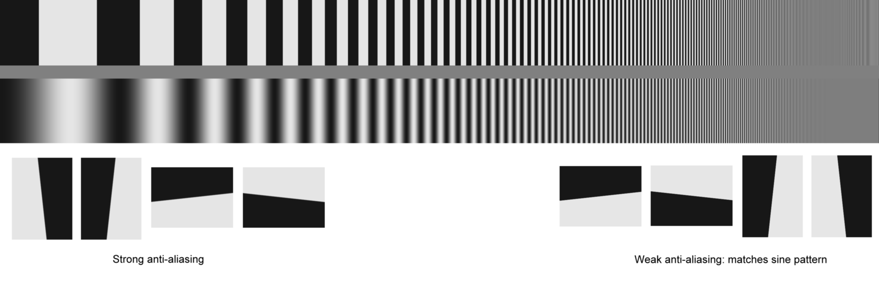
Blur More pattern. Click to download full-sized image.

Blur More sine pattern MTF results

Blur More slanted-edge MTF results
MTF up to 0.35 Cycles/Pixel is nearly identical. The summary values, MTF50, MTF20, and MTF10, are all very close.
3. Gaussian Blur Radius = 2 (strongly blurred)
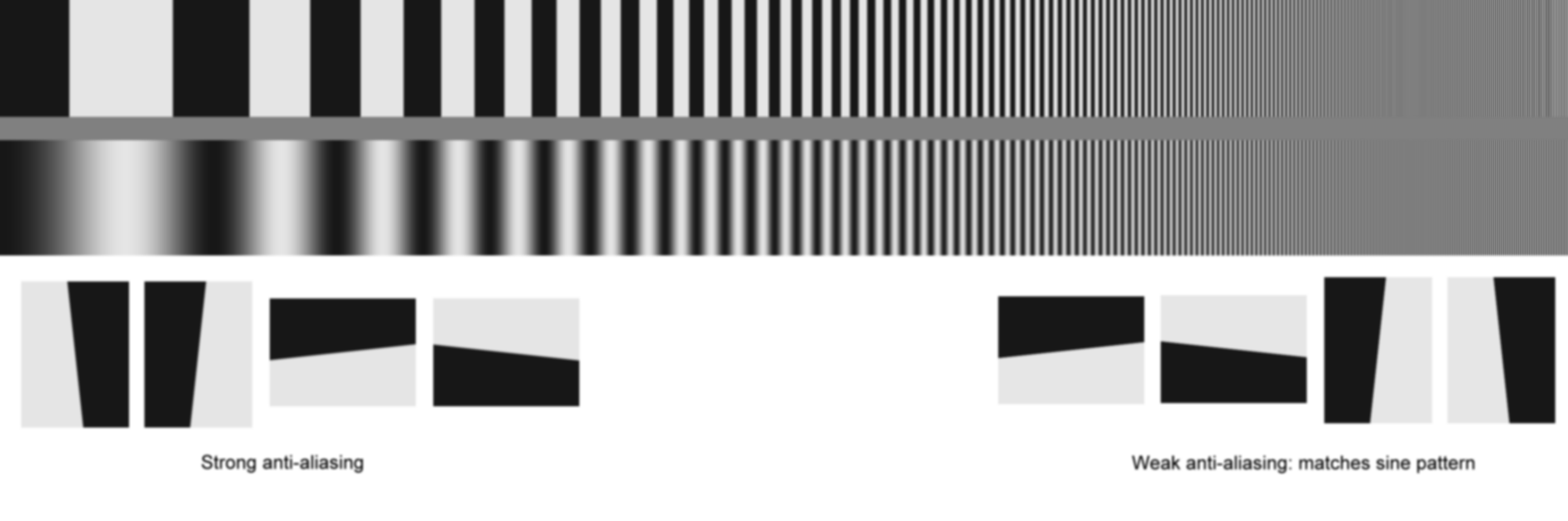
Gaussian-blurred (Radius = 2) pattern. Click to download full-sized image.
 Gaussian Blur R=2 sine pattern MTF results

Gaussian Blur R=2slanted-edge MTF results
Again, these plots and the summary values derived from them are close to identical.
Verification using the sine pattern
To further verify the results, let’s look at the original sine pattern for the BlurMore case, which is displayed below by the Imatest Log Frequency module.

Blur more pixels (the two plots are the same because gamma = 1)
This sine pattern can be viewed by ImageJ, a widely-used program developed by the National Institutes of Health that can be downloaded from http://rsbweb.nih.gov/ij/. The use of ImageJ for analyzing a sine pattern is described on http://normankoren.com/Tutorials/MTF5.html#ImageJ (quite an old web page; predating Imatest). To summarize: Run ImageJ, then open the test image with File, Open. Select the line tool (shown below) and use the mouse to draw a horizontal line along the portion of the image you wish to analyze (the sine pattern).

ImageJ window

ImageJ selection
Note that the spatial frequency increases logarithmically from left to right. After you’ve drawn the line, click on Analyze, Set Scale… Distance in Pixels should be nonzero. The width of the image in pixels (approximately 2950, shown on the right) or 1 are good numbers to use. Unit of Length: can be anything as long as it’s not blank. Pixel is a good choice. Click OK. Then click Analyze, Plot Profile. The window below appears.

ImageJ output
This window is not terribly useful because it’s a bitmap; hence enlarging it does not increase the detail. Fortunately you can click on then paste the results into column A1 of Excel. This puts Distance (Pixels) in column A and Gray value (i.e., pixel level) in column B. The Excel file used to produce the plots shown below is included along with the image files. Excel formulas have been used to normalize the response to ±0.5 at low spatial frequencies. There equations are:
Column A contains the location. Not used. Column B contains the Pixel level. H1: =AVERAGE(B1000:B2949) I1: =MAX(B:B)-MIN(B:B) Column C: =(B:B-H1)/I1
At MTF50 (the spatial frequency where MTF is 50% of the low frequency value; used for comparison with Imatest results) the pattern below, which is from Column C, varies between ±0.25.  After a bit of trial-and-error we enlarged the portion of the plot around MTF50.
  The region where the envelope is close to ±0.25 is between the peaks at 72 and 97, which comprise 5 complete cycles. (We could have used any reasonable number from 4 to 10 cycles.) The spatial frequency is MTF50 = 5/25 = 0.20 Cycles/Pixel. This can be compared with Imatest BlurMore results, above: 0.21 C/P from the sine pattern and 0.202 C/P from the slanted-edge. This is a strong verification that the Imatest slanted-edge calculation is in excellent agreement with an independent first-principles measurement.
Acutance and SQF (Subjective Quality Factor)
Acutance and SQF are measurements of perceived sharpness as a function of print or display height and viewing distance (they are actually angular calculations). They require an assumption about viewing distance (can be constant or proportional to the square root or cube root of print height). Acutance and SQF includes the effects of
- MTF: the imaging system’s Modulation Transfer Function (synonymous with Spatial Frequency Response (SFR)),
- CSF: the human eye’s Contrast Sensitivity Function,
- print height, and
- viewing distance
Validation of Acutance and SQF
SQF measurement does not conform to any widely-recognized standard. It was used internally in Kodak and Polaroid starting in the 1970s, and it is used for Popular Photography lens test reports. Acutance, on the other hand, has been the subject of a significant amount of verification work correlating Acutance measurements to JNDs (Just Noticeable Differences). This work is described in the set of documents, “CPIQ 2.0 Specifications & Test Methods, which includes: Acutance SFR, Color Uniformity, Lens Geometric Distortion, Chromatic Aberration & Subjective Evaluation methods”, see our CPIQ support page for details.