Contrast Detection Probability (CDP) Background
By definition, luminance contrast is the relationship between a bright area and an adjacent dark area. The contrast is subject to change, depending on various factors such as the imaging system being used, observer’s perception, illumination, distance from the target, and ambient room lighting. The contrast requirements of an imaging system must be fulfilled based on the total range of density values recorded on the image. Therefore, the imaging chain has to guarantee that a specified contrast can be detected in the signal by a given probability. Produced and to be reviewed by the IEEE p2020 Automotive Image Quality standards committee, the contrast detection probability (CDP) allows each contrast measurement result to be expressed inside confidence intervals with given probabilities. (For more information, refer to Detection Probabilities: Performance Prediction for Sensors of
Autonomous Vehicles.1)
The CDP in Imatest is defined from one of two contrast metrics—the Weber contrast and the Michelson contrast:
- The Weber contrast \(C_{W} \) metric is based on the Weber-Fechner law on human perception. The contrast measures the difference between the high and low luminances (L) divided by the lower luminance:
\(C_{W} = \frac{L_{max}-L_{min}}{L_{min}} = \frac{L_{max}}{L_{min}}-1 \) - The Michelson contrast \(C_{M} \) metric is more common in the optics field. It measures the relationship between the spread and the sum of the two luminances:
\(C_{M} = \frac{L_{max}-L_{min}}{L_{max}+L_{min}} \)
Imatest’s implementation of CDP is the integral of the probability of observing a contrast.
\(CDP=\displaystyle\int_L^H{pdf}_C\mathrm{d}c\)
This allows for investigations of CDP behavior with different sets of bounds. Bounds where the upper limit is infinite for Weber or 1 for Michelson contrasts enable investigation if the system can replicate (or enhance) a scene contrast.
Imatest CDP
CDP measurements in Imatest 5.2 require a contrast resolution test chart illuminated by a backlit light source such as the Imatest LED Lightbox. When navigating through the Color/Tone Interactive module, there are two display options available for visualizing and analyzing the CDP: 1) CDP details plot and 2) CDP summary plot, both of which are available in the Color/Tone Interactive and the Color/Tone Auto modules.
Imatest 5.2 (or later) can produce CDP measurements using the Contrast-Resolution test chart via low contrast objects in a variety of contexts from bright to dark, challenging the imaging system to get appropriate exposures of a wide range of tones (see chart below).
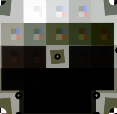
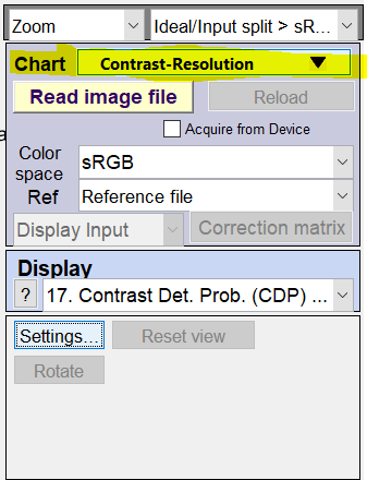
To generate the CDP results in Imatest (see Contrast-Resolution chart above), do the following:
- Choose the Color/Tone Interactive module.
- Select the drop-down button in Charts.
- Click Grayscale charts.
- Select Contrast-Resolution (see below).
CDP Display Options
There are two main CDP Display options available in Imatest: 1) CDP Detail and 2) CDP Summary. Both display options are addressed below.
CDP Detail (Display#17)
The first display option is the CDP Detail, which can be found by navigating to Display#17 in the color/tone interactive display option. A sample image of the CDP detail plot is shown below.
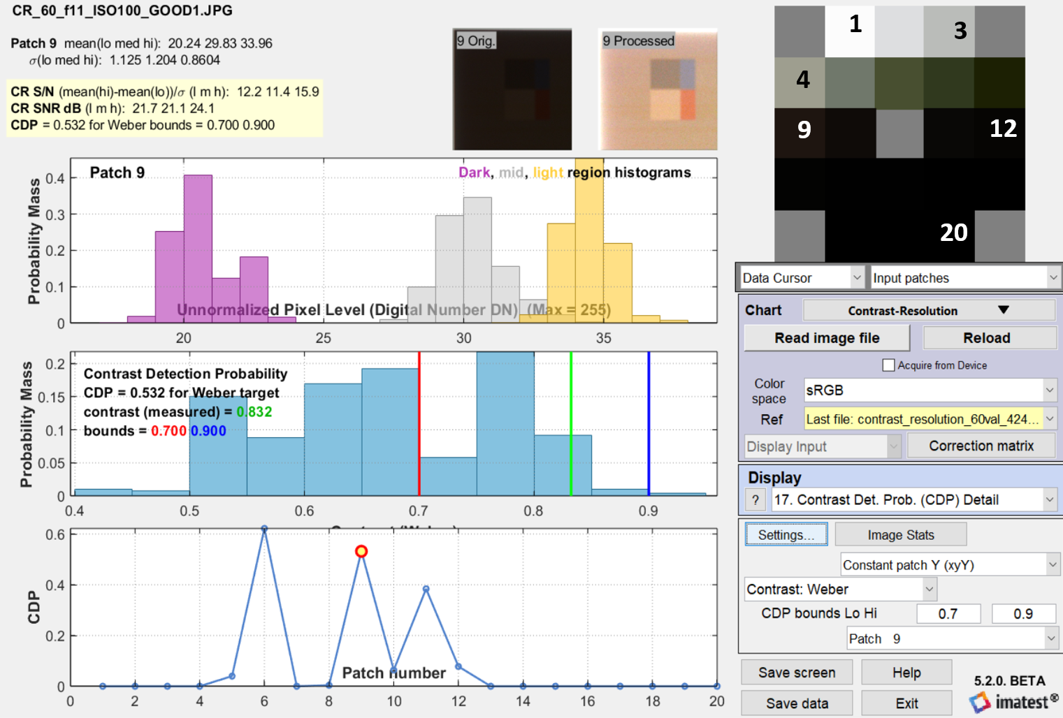
The CDP plot allows the user to visualize each patch in the contrast-resolution chart separately. Shown above is Patch 9 in the given Contrast-Resolution chart. Notice on the right side of the above figure, the contrast is set to Weber. The user can measure contrast using Weber or Michelson contrast metrics. Both values are rescaled to match one another; in this way, the final CDP plot results will not change.
Imatest CDP measurement
Imatest allows the user to set the lower and upper bounds for all the patches and select either Cw or Cm contrast. The red and blue lines (in the middle subplot) correspond to the “CDP bounds Lo Hi” user-specified parameters. The parameter values are based on the application of the imaging system and the contrast of the patch of interest.
In this context, the contrast was set between 0.7 and 0.9 for Patch 9. The contrast of the chart based on the associated reference file is 0.8332 (green line). All the contrast values within the specified bounds are then integrated to quantify the CDP.
Subplots of CDP Detail (Display#17)
The upper subplot represents the histogram of the user-selected patch, in this case Patch 9:
- The purple bins (dark) correspond to the black region within the patch.
- The gray (mid) bins correspond to the background of the patch.
- The yellow (light) bins correspond to the white region within the patch.
The x-axis represents the DN of the patches (if desired, it can be normalized in the settings), while the y-axis represents the normalized probability mass occurrence of the corresponding luminance region (dark, mid or light) within the patch selected.
The middle subplot shows the histogram of the Weber or Michelson (Weber was used in the above figure) metrics. The x-axis represents the Weber or Michelson contrast value. The y-axis represents the normalized probability mass occurrence of the corresponding patch. The values in the middle plot that are within the bounds are integrated and a CDP metric is then calculated. This process is done for every patch in the Contrast-Resolution chart. The bottom subplot shows the measured CDP of each patch.
CDP Summary (Display#18)
Display#18, shown below, provides a brief CDP summary for all the contrast resolution patches.

For each patch, the following measurements are displayed:
- The top value shows the CDP measurement.
- The middle value displays the corresponding patch number.
For more information on Contrast Resolution, please refer to our Contrast Resolution chart and analysis page.
JSON outputs
This shows each pair of CDP calculations for the 20-patch contrast resolution chart:
“Contrast_Detection_Probability”: [1,1,1,1,0.96,0.846,0.944,0.892,0.734,0.654,0.404,0.292,0.26,0.136,0.086,0.07,0.066,0.056,0.044,0.038],
References
- Geese, M., et al. “Detection Probabilities: Performance Prediction for Sensors of Autonomous Vehicles.” Electronic Imaging, vol. 2018, no. 17, 2018, doi:10.2352/issn.2470-1173.2018.17.avm-148.
- Artman, U., et al. “Contrast Detection Probability – Implementation and Use Cases.” Electronic Imaging, Autonomous Vehicles and Machines Conference 2019, Pp. 30-1-30-13(13), 13 Jan. 2019.