Documentation
by Norman Koren
© 2009 Imatest LLC
Imatest Documentation
Image Quality
Sharpness - What is it and how is it measured?
SQF - Subjective Quality Factor
Sharpening - Why standardized sharpening is needed for comparing cameras
Imatest Instructions
MTF Compare - Compare MTFs of different cameras and lenses
Batchview - Postprocessor for viewing summaries of SFR, SFRplus results
Dynamic Range - Calculate Dynamic Range from several Stepchart images
Log F-Contrast - Analysis of charts that vary in log frequency and contrast
Using Print Test - Measure print quality factors: color response, tonal response, and Dmax
Maskfill - Removes features that interfere with Imatest measurements
Appendix
License - The Imatest End User License Agreement (EULA)
Tour of Imatest
Tour of Imatest
Brief tour of highlights
Imatest™
is a suite of programs for measuring the sharpness and image quality of lenses,
digital cameras, digitized film images, and prints using inexpensive, widely available
targets. It is available in three versions:
Modules
Imatest consists of several modules, each of which analyzes images of one or more test charts. Image files can be in any of several standard formats (TIF, high quality JPEG, PNG, etc.). Imatest Master also analyzes Bayer RAW files. A Test chart Cross-reference follows.
 |
SFR measures the sharpness of cameras and lenses using a simple slanted-edge target (either the industry-standard ISO
12233 chart or a target you can print yourself on a high quality
inkjet printer). Its standardized
sharpening algorithm allows you to compare digital
cameras on a fair basis. It also analyzes Chromatic Aberration and noise and calculates the Subjective Quality Factor (SQF)— a measurement of how sharp a print of a given size will appear, based on MTF and the eye's Contrast Sensitivity Function (CSF). It can analyze regions as small as 10x10 pixels. |
 |
MTF Compare (Imatest Master only) is a post-processor for Imatest SFR that compares the MTFs of different cameras, lenses, and imaging systems using saved data from CSV files. These comparisions are far more detailed than comparisions of MTF50 or other summary results. |
 |
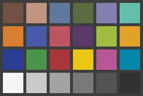
Colorcheck
measures a camera's color quality, tonal response, exposure accuracy, and noise
using the GretagMacbethTM
ColorChecker®, which is available from Adorama and other sources. |
 |
Stepchart
measures a camera's
tonal response, noise, and dynamic range using grayscale step charts from Kodak (the Q-13/Q-14), Jessops, or Danes-Picta (Czech Republic), or transmission step wedges
from Stouffer, Danes-Picta,
or Kodak. It also measures exposure accuracy and veiling glare (susceptibility to lens flare) with reflection step charts. It also works with several charts (some ISO standards) from Applied Image. The Dynamic Range postprocesser for Stepchart, measures dynamic range from Stepchart results for several differently-exposed stepchart images. |
 |
Multicharts analyzes several color charts for tonal response and color accuracy using a highly interactive interface. It also analyzes grayscale charts for tonal response. It currently supports the standard 24-patch GretagMacbethTM ColorChecker® and the IT8.7 in Imatest Studio and Master and the ColorChecker SG, several linear grayscale stepcharts, and patterns of squares arranged on a circle (for analyzing custom "pie" charts) in Imatest Master. |
 |
Print Test measures the quality (color response, color gamut, tonal response, and Dmax) of printers, inks, paper, ICC profiles, and rendering intents. A version of Print Test with additional capabilities is included in Gamutvision. |
|
Light Falloff (Uniformity) measures the light falloff (vignetting) of lenses. In Imatest Master it also measures several types of image sensor nonuniformity, including color shading, detailed noise distribution, and medium-sized (visible) nonuniformities, inculding dust smudges. It also flags stuck (dead and hot) pixels. A histogram display makes it easy to select dead/hot pixel thresholds. Display options include contours superposed over images and pseudocolor with color bar. |
|
Distortion measures lens distortion and calculates coefficients for correcting it using a square or rectangular grid that can be printed from files created by Test Charts. |
 |
Rescharts analyzes several resolution-related test charts using a highly interactive interface. Functions include Slanted-edge SFR, which largely duplicates the calculations in SFR, Log frequency, which measures MTF and color moiré using a chart that varies in spatial frequency, and Log frequency-contrast (Imatest Master only), which measures MTF and loss in fine detail due to software noise reduction using a chart that varies in spatial frequency on one axis and contrast on the other. |
|
Test Charts creates image files for printing test charts on high quality inkjet printers. Charts include SFR slanted-edge images, star charts, patterns with varying spatial frequency and contrast, and zone plates. Several patterns can be used for observing aliasing, Color Moire, detail lost to software noise reduction, and other phenomena. Numerous options are available, including contrast ratio, highlight color, and sine or bar pattern (for certain charts). Both bitmap and Scalable Vector Graphics (SVG) charts, which can be printed any size without loss of quality, are available. |
 |
Concise instructions for testing lenses using Imatest SFR. |
 |
Gamutvision is a standalone program (sold separately from Imatest) for exploring the behavior of color management, gamut mapping, and rendering intents, incorporating Print Test. See precisely how gamut mapping affects colors. Assess ICC profile quality. Learn how working color space affects print quality. Determine the capabilities of printers and papers using downloaded ICC profiles. Compare them with scanned prints from your own printer. And much more... |
| Imatest is frequently updated. Major releases are announced on the Imatest main page. All releases are described in detail in the Change Log. You can download and install a new version at any time without uninstalling the old version. |
| Imatest is written in compiled Matlab, Release 13 (Version 6.5.1), an outstanding language for solving
engineering problems. Algorithms can be rapidly coded and modified
in response to user requests. It is a standalone program; Matlab does not need to be installed, but the Matlab runtime library needs to be downloaded and installed once (the first time Imatest is installed). In most cases this is done automatically. |
| Requirements: Windows 2000, 2003, XP, Vista, or later, or Macintosh computers with Virtual PC 6 or 7. Minimum RAM is 256 MB (512 MB recommended), and minimum screen size is 1024x768 pixels. |
| Supported input file formats: TIFF, PNG, or PPM (all 24 or 48-bit), JPEG, BMP, GIF, HDF, PCX, XWD, as well as RAW files from most digital cameras, using Dave Coffin's dcraw. |
| Imatest output is optionally written to two types of file: .CSV (comma-separated variable; Excel-readable), and XML. |
 |
To run Imatest in Windows Vista, you'll need version 2.3.3 or later. |
|
Test chart cross-reference
The table below lists commercially-available charts. Additional charts that you can print a high quality inkjet printer are described in Test Charts. Cross references contains this material sorted by quality factor and module.
| Chart |
Quality factor |
Module |
Comments |
| ColorChecker SG |
Color accuracy, Tonal response |
Multicharts |
Imatest Master only. |
| Custom "pie" charts |
Color accuracy, Tonal response |
Multicharts (Special charts) |
Imatest Master only. |
| GretagMacbeth ColorChecker (24-patch) |
Color accuracy, Tonal response, Noise |
Colorcheck, Multicharts |
Widely available; consistent pigments |
| ISO 12233, Applied Image QA-77 |
Sharpness, Lateral chromatic aberration, Subjective Quality Factor (SQF) |
SFR |
Printed on high resolution photographic media. Slanted-edge charts printed on a high quality inkjets can perform the same function, but aren't as fine. |
| IT8.7, CMP (Christophe Metairie Photographie) DigitaL TargeT 003 (CMP DT003), QPcard 201 |
Color accuracy, Tonal response |
Multicharts |
IT8.7 and CMP DT003 require reference file (supplied with target) |
| Monochrome charts: ISO-16067-1, QA-62, EIA Grayscale, ISO-14524
OECF, ISO-15739
Noise |
Dynamic range, Tonal response, Contrast |
Stepchart, Multicharts (Special charts) |
Imatest Master only. Most are available from Applied Image. |
| Step charts (reflective): Kodak Q-13, Q-14, etc. |
Tonal response, Contrast, Noise, Exposure accuracy, Veiling glare |
Stepchart, Multicharts |
|
| Step charts (transmissive): Stouffer T4110, etc. |
Dynamic range, Tonal response, Contrast, Noise |
Stepchart |
Best for measuring dynamic range |
Try
Imatest
You can download an evaluation version that allows you to make up to 20 runs of the individual
modules. It has all the capabilities of the full versions except that
(1) you can't save results, and (2) a watermark appears in the background
of the figures.
You may purchase Imatest at any time by from our secure online store
by going to the purchase page. The price includes one year of updates. You may also purchase Imatest via wire transfer or custom Paypal invoice. You can register Imatest
as soon as the purchase is complete. Details can be
found on Installing Imatest and getting
started.
Learn
more about Imatest
All
Imatest documentation is available online. The Documentation page contains the table of contents, and the Cross-reference indexes image quality factors, modules, and test charts. The FAQ answers many questions.
Many of the
concepts used by Imatest to
measure sharpness and image quality are new to photographers and require some study. Sharpness: What is
it and how is it measured? is a good place to start. It outlines
the basic principles behind SFR. Standardized sharpening:
why it's needed for comparing cameras, Chromatic
aberration, and Subjective Quality Factor (SQF)
contain additional concepts. Shannon information capacity is a relatively new concept for imaging, still under development— its measurement is distorted by ubiquitous software noise reduction.
Using
Imatest contains instructions that are common to all modules. Instructions for SFR, Colorcheck, Stepchart, Print test, and additional modules are on individual pages.
Many of the terms used in the documentation are defined in the Glossary.
An Imatest
forum has been established for posting questions and responses. The Change Log describes the Imatest version.
The
Imatest license
The Imatest license for Light and Pro allows an individual user to register and use the software on (A) a maximum of three computers (for example, home, laptop,
and office) used exclusively by a single individual, or (B) a single workstation
used nonsimultaneously by multiple people, but
not both. It is not a concurrent use license. The full license may be viewed here.
License holders are encouraged to publish test results in printed publications,
websites, and discussion forums, provided they include links to www.imatest.com.
The use of the Imatest Logo is encouraged. However you may not use Imatest
for advertising or product promotion without the explicit permission of
Imatest LLC. Contact us to learn more.
Imatest LLC assumes no legal liability for the contents of published
reviews. If you plan to publish test results, you should take care to use
good technique. See Using
Imatest for more details.
Links
Volker Gilbert has written an excellent French language description of Imatest. (PDF version)
Colorcheck
Colorcheck analyzes images of the GretagMacbeth ColorChecker for tonal response, gamma, noise, and color fidelity.
Colorcheck:
color accuracy and tonal response
Imatest™ Colorcheck analyzes images of the X-Rite (formerly GretagMacbethTM ) ColorChecker® for color accuracy, tonal response, gamma, and noise. It is particularly useful for measuring the effectiveness of White Balance algorithms and settings under a variety of lighting conditions. The ColorChecker is available from ColorHQ, Adorama, and other suppliers.
You can select the Colorchecker reference values (using standard values or the contents of a data file) and one of six color spaces: sRGB, Adobe RGB (1998), Wide Gamut RGB, ProPhoto RGB, Apple RGB, or ColorMatch. Danny Pascale/Babelcolor's page on the Colorchecker contains nearly everything you want to know about the chart.

To run Colorcheck, photograph the ColorChecker, taking care to avoid glare. For best results, the chart image should be 500-1500 pixels wide, though smaller images produce satisfactory results. For testing white balance, you can photograph a ColorChecker in a scene. The ColorChecker image can be very small if a noise analysis is not required. Load the image file, crop it (if needed), then make any needed changes to the input dialog box (for color space, which defaults to sRGB, etc.).
The first figure: gray scale analysis
shows the tonal response and noise of
the gray patches at the bottom of the Colorchecker and and selected EXIF data..
The upper left plot shows the pixel levels of the
six patches. Gamma (the exponent of the equation that relates scene luminance to pixel level) is defined by the
first order fit (the dotted blue line). |
|
The upper right plot is the transfer curve
(with similar scaling to film transfer curves): the density (log(Pixel
level/255)) as a function of Log exposure ( (-) target density). Stepchart produces a more detailed transfer curve. It also shows the exposure error. The best results are obtained if it is kept under 0.25 f-stops. Note that the x-axis scale (log exposure) is reversed from the plots on the left. |
The lower left plot shows the R, G, B, and Y (luminance) noise, normalized to the difference
between the white and black patches (a density difference of 1.45). Several additional options are available for displaying noise or SNR (Signal-to-Noise Ratio). |
|
The lower right region displays EXIF data, if
available. |
The
second figure: noise detail (Imatest Master only)
shows the density response, noise in f-stops (a relative measurement
that corresponds to the workings of the eye), noise for the third
Colorchecker row, which contains primary colors, and the noise spectrum of the selected patch.
The upper left plot is the density
response
of the
colorchecker (gray squares). It includes the first and second order
fits
(dashed blue and green lines). The horizontal axis is Log Exposure (minus the target
density), printed on
the
back of the ColorChecker. Stepchart provides a more detailed
density response curve. It also shows exposure error in f-stops. |
|
The upper right plot shows the noise in the
third colorchecker row, which contains the most strongly colored
patches: Blue, Green, Red, Yellow, Magenta, and Cyan. In certain
cameras noise may vary with the color. Problems may be apparent that
aren't visible in the gray patches. Several options are available for displaying noise or SNR (Signal-to-Noise Ratio). |
The lower left plot shows the R, G, B, and Y
(luminance) RMS noise or SNR as a function of Log Exposure
each patch. Any of several displays may be selected. The above figure has RMS noise is expressed in f-stops, a relative measure that
corresponds closely to the workings of the human eye. This measurement
is described in detail in the Stepchart tour. It is largest in the dark areas because the pixel
spacing between f-stops is smallest. |
|
The lower right plot shows the noise
spectrum for the R, G, B, and Y channels for the selected patch. An unually rapid dropoff may indicate a large amount of noise reduction software,
which can mask fine detail. |
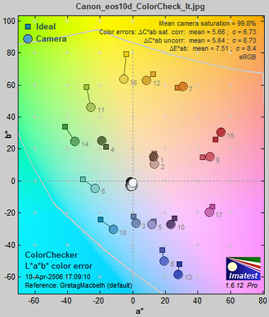
The third figure: color error
shows the color error (the difference between the measured and ideal (reference) values)
in the a*b* plane of the CIELAB color space, which is relatively perceptually
uniform (not perfect, but far more uniform than the common xy Chromaticity
diagram). The small squares are the ideal values; the large circles are
the measured (camera) values. The chroma (related to the perception of saturation) of an individual color is
proportional to its distance from the origin (a* = b* = 0).
The mean camera
chroma (the average of all camera chroma values) relative to the
mean ideal chroma is displayed on the upper right. You can select one of three color error metrics: ΔE*ab (CIE 1976; the familiar Euclidian distance), ΔE*94 (CIE 1994), and ΔE*CMC. ΔE*94 and ΔE*CMC are more complex but more accurate. Mean and RMS (root mean square; σ) or maximum color errors (measured with and without a correction for camera chroma boost or cut) can be displayed. RMS error gives more weight to large errors. Calculation details are given in the Colorcheck Appendix.
|
|
Images can be analyzed in sRGB, Adobe RGB (1998), Wide Gamut RGB, ProPhoto RGB, Apple RGB, and ColorMatch RGB color spaces. The light gray curve is the boundary of the sRGB color space.
|
| When you interpret the results, keep the following in mind.
Camera manufacturers do not necessarily aim for accurate color reproduction, which often appears flat and dull. They recognize that there is a difference between accurate and pleasing color: most people prefer deep blue skies, saturated green foliage, and warm, slightly saturated skin tones. Ever mindful of the bottom line, they aim to please.
Hence they often boost chroma (i.e., saturation), especially in blues, greens, and skin tones. |
Colorcheck can be used to check white balance algorithms and camera performance under different lighting conditions. John Beale's excellent article on Lighting and Color uses this Colorcheck figure to examine the effects of different lighting on color accuracy. |
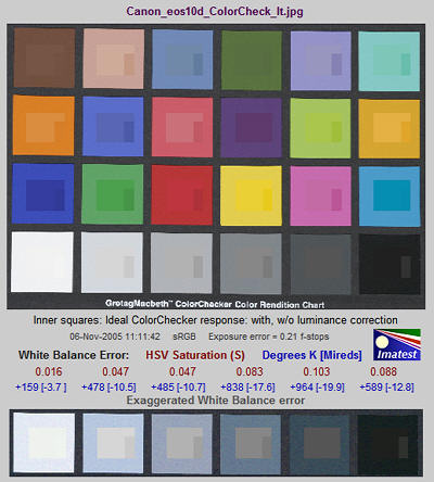
The fourth figure: color analysis
is an image of the ColorChecker with the correct colors superposed in the center of each patch. The colors in the central squares are corrected for the difference in luminance between the exposed and the ideal values. The colors in the small rectangles to the right of central squares are uncorrected.
The gray patches with exaggerated White Balance error are shown on the bottom. White balance error is displayed in HSV Saturation units, degrees Kelvin, and Mireds (1000/degrees K; a useful unit for filtration). |
 |
|
|
GretagMacbethTM and ColorChecker® are tradmarks of X-Rite, Incorporated, which is not affiliated with Imatest. ColorChecker L*a*b* values are supplied courtesy of X-Rite.
Stepchart
Measures tonal response, noise, and dynamic range using step charts
Imatest™ Stepchart
analyzes the tonal response, noise,
and dynamic range of digital
cameras and scanners using
Stepchart can also measure veiling glare (lens flare) using reflection step charts. Results are more detailed than those provided by Colorcheck. Transmission step charts are recommended for measuring dynamic range. Full instructions can be found on Using Stepchart. Noise is explained in Noise in photographic images.
| To run Stepchart, photograph the chart, taking care to avoid glare (shiny reflections). Scale the image for 50 pixels per zone for greatest noise analysis accuracy; 20 pixels per zone is adequate in most cases. Fewer are OK for tonal response curves. Load the image file, crop it (if needed), then specify the target density step and type (reflective or tramsmission). The default is a reflective target with density step = 0.1. |
 |
The two Figures below illustrate the results of analyzing a Q-13 image photographed with the Canon EOS-10D at ISO 100. A third figure (not shown here) displays density response for all channels (Y, R, G, and B) in color images.
The first figure
contains basic tonal response and noise measurements.
The horizontal axis for both plots is the chart zone— proportional to the distance along the chart. Density (–Log Exposure) increases by a fixed step (0.10 or 0.15, depending on the target) for each zone.
The upper plot
shows the normalized pixel level of the
grayscale patches (black curve) and first and second order
density fits (dashed blue and green
curves). Gamma is derived from the first order fit. The acvite areas used for the analysis is shown as think pale pink bars.
The lower plot shows the RMS noise for
each patch:
R, G, B, and Y (luminance), expressed as the percentage of the pixel level difference corresponding to a target density range of 1.5: the same
as
the white - black patches on the GretagMacbeth ColorChecker. For this camera, the pixel difference is 197.5. Noise measured in pixels can be calculated by multiplying the percentage noise by 197.5. Noise can also be normalized to the maximum pixel level (255). The average noise for each channel (excluding the lightest and darkest zones) is displayed. See Noise in photographic images for a detailed explanation of noise.
|
 |
The second
Figure
contains the
most important results:
- the response curve displayed on a log
scale, similar to film response curves,
- noise expressed units of f-stops (the same as EV), explained below, or SNR (Signal-to-Noise Ratio), explained here,
- noise in normalized pixel levels
- dynamic range (for
transmission step charts),
- the noise spectrum.
The horizontal
axis for the three plots is Log Exposure, which equals
(–) the nominal target
density
(0.05 - 1.95 for the Q-13/Q-14). This axis is reversed from Figure 1.
The upper left plot shows the density response (gray squares), as well as the first and second order fits (dashed blue and green lines). It resembles a traditional film density response curve. Dynamic range is grayed out because the reflective Q-13 target has too small a dynamic range to measure a camera's total dynamic range. See Dynamic range, below. This curve is sometimes called the Opto-Electronic Conversion Function (OECF). |
The upper right box contains dynamic range results: total dynamic range and range for several quality levels, based on luminance (Y) noise. It is shown in gray when a reflective target is selected. |

The middle left plot shows
noise in f-stops or EV, i.e., noise scaled to (divided by) the
difference in pixel levels between f-stops, which decreases as
brightness decreases. The darkest levels have the highest f-stop noise.
This
measurement corresponds to the response of the eye and has
important consequences for the calculation of practical dynamic range.
The vertical axis is logarithmic for clear display of low noise values.
This plot can also be displayed as SNR (Signal-to-Noise Ratio; shown below), which is the inverse of f-stop noise.
|
EXIF data is shown in the
middle right region (JPEG files only).
|
The bottom left plot
shows the noise scaled to the difference in pixel levels between the
maximum density level and the patch corresponding to a density of 1.5—
the same density range as the GretagMacbeth Colorchecker. Several additional options are available for displaying noise or SNR (Signal-to-Noise Ratio).
|
The lower right plot
shows the noise
spectrum. Digital
camera images with excessive noise reduction will have an unusually
rapid
falloff of the noise spectrum. When combined with the eye's contrast sensitivity function (CSF), the noise spectrum can be used to calculate the visiblity of noise. |
SNR (S/N = 1/f-stop noise),
in middle-left plot
in
place of f-stop noise.
|
 |
Why measure noise in f-stops?
Because the human eye responds to relative luminance differences. That's why we think of exposure in terms of zones, f-stops, or EV (exposure value),
where a change of one unit corresponds to halving or doubling
the exposure.
The eye's relative sensitivity is expressed by the Weber-Fechner
law,
ΔL ≈ 0.01 L –or– ΔL/L ≈ 0.01
where ΔL is the smallest luminance difference the eye can distinguish. (This equation is approximate; effective ΔL tends to be larger in dark areas of scenes and prints due to visual interference from bright areas.)
|
 |
Expressing noise in relative luminance units, such as f-stops, corresponds more closely to the eye's response than standard pixel or voltage units. Noise in f-stops is obtained by dividing the noise in pixels
by the number of pixels per
f-stop. (I use "f-stop" rather than "zone" or "EV" out of habit; any of them are OK.)
noise in f-stops = noise in pixels / (d(pixel)/d(f-stop)) = 1/SNR
where d(pixel)/d(f-stop) is the derivative of the pixel level with respect to luminance measured in f-stops (~log2(luminance) ).
SNR is the Signal-to-Noise Ratio. |
The above-right image illustrates how the pixel spacing between f-stops (and hence d(pixel)/d(f-stop)) decreases with decreasing brightness. This causes f-stop noise to increase with decreasing brightness, visible in the middle-left plot of the second figure, above.
Since
luminance noise (measured in f-stops) is referenced to relative scene luminance,
independently of electronic processing or pixel levels, it is a universal measurement
that can be used to compare digital sensor quality when sensor RAW data is unavailable. |
Dynamic
range
| The new Dynamic Range module calculates dynamic range from several reflective stepchart images, which are easier to work with than transmission step charts. |
|
Dynamic
range is the range of brightness over which a camera responds. It is
usually measured in f-stops, or equivalently, zones or EV. It can
be specified in two ways:
- The total range.
Stepchart measures a camera's total dynamic range, including noisy dark areas.
- A range of tones over which the RMS noise, measured in f-stops, is under a maximum
specified value. The lower the maximum noise value, the better the
image
quality, but the smaller the dynamic range. Noise tends to be worst in
the darkest regions. Imatest calculates the
dynamic range for several maximum
noise levels, from RMS noise = 0.1 f-stop (high image
quality) to 1 f-stop (relatively low quality).
Change in dynamic range definition (Imatest 1.5.5, November 24, 2005)
The definition of total dynamic range now includes indistinct zones (dark zones that the original Stepchart algorithm had difficulty detecting). This may cause some short-term confusion because Figure 2 will change: total DR will sometimes increase. But it better represents true camera performance. |
|
Dynamic
range is measured using transmission
step charts, which have density
ranges of at least 3.0: a 1000:1 ratio (10 f-stops). Reflective
charts such as
the
Q-13 have a density range of only around 1.90; an 80:1 ratio (6.3
f-stops), insufficient for digital cameras. Two charts are recommended for digital SLRs, which can have over 10 f-stops of total dynamic range.
- The Stouffer T4110 transmission step wedge, which has a maximum density of 4.05 (41 steps, 0.1 density increment, 13.3 f-stops dynamic range)
- The Danes-Picta TS28D (on their Digital Imaging page), which has a maximum density of 4.2 ( 28 steps, 0.15 density increment, 13.6 f-stops dynamic range)
The dynamic range is the difference in density between the zone where the pixel level is 98% of its maximum value (250 our of 255 for 24-bit color), estimated by interpolation, and the darkest zone that meets the measurement criterion. The repeatability of this measurement is around 1/3 f-stop.
The
figure below illustrates results
for the Canon EOS-10D,
taken from a JPEG image acquired
at ISO 400 and converted with Canon Zoom Browser set for low contrast.
A Kodak step tablet (density from 0.05 to 3.05 in steps of 0.15) was
used.
The total dynamic
range is 8.58 f-stops (probably limited by the target; the Stouffer T4110 or Danes-Picta TS28D would have done a better job). It is displayed at the bottom of the upper-left plot (Density response). Total dynamic
range changes little for 48-bit TIFF conversion or ISO 100. But 48-bit
TIFF conversion has lower noise, hence higher dynamic range at any given
quality level.
A medium quality image can ge achieved over a range of 8.21 f-stops out of a total dynamic range of 8.58 f-stops. When a high quality image is required (maximum noise = 0.1 f-stops),
the dynamic range is reduced to 5.97 f-stops (indicated by the yellow line on the middle left plot). The best slide
films have a total dynamic range of 5 to 6 f-stops.
The
second plot contains all important Stepchart results.
The shape of the response curve
depends
strongly on the conversion software and settings.
Compact digital
cameras have much higher noise levels, hence lower useful dynamic
range, even though their total dynamic
range may be quite
large. Roger N. Clark, a space scientist and avid photographer has done a study of dynamic range. He finds digital (SLRs) to be superior to film.
Scanner results
Here are the results of scanning the Kodak step
tablet with the Epson 3200 scanner (with transparency unit) set for negatives.
A few
observations on the scanner results:
- All 20 steps of the Kodak step tablet were detected. The total
dynamic range is greater than 3 density units (the 10 f-stop range
of the tablet). To determine the true total dynamic range we would need the Stouffer T4110 step wedge,
which has a maximum density of 4.
- The response closely follows an exponential curve with gamma =
0.506. No "S" curve has been superposed.
- The practical dynamic range is limited by noise. It is 9.62
f-stops (2.9 density units) for a medium quality image.
- The flat noise spectrum indicates that no software noise
reduction has been applied. Most digital cameras have rolloffs in their noise spectra due to Bayer interpolation and noise reduction.
SFR
Measures image sharpness using a slanted-edge target
SFRplus
Automated measurement of image sharpness and other quality factors
Imatest™ SFRplus
measures image
sharpness and several additional image
quality factors,
including Lateral Chromatic Aberration (LCA), noise, distortion and tonal response, using a special test chart that provides a high degree of automation.
The primary sharpness indicator is MTF50, the spatial
frequency
where contrast drops to half its low frequency value.
Spatial Frequency Response (SFR), also known as Modulation Transfer Function (MTF), is introduced in What
is image sharpness and how is it measured?
Full instructions for using SFRplus and interpreting its results can be found in Using SFRplus Part 1: Setup, Part 2: Running, and Part 3: Results.
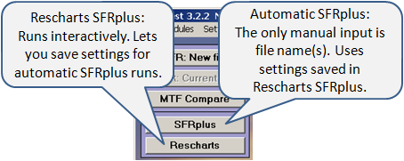
SFRplus runs in two modes.
To use SFRplus,
- Purchase an SFRplus test chart and mount it on a rigid substrate (typically 1/2 inch foam board).
|
 |
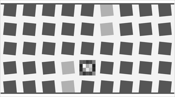
Standard SFRplus test chart: 5x9 grid, 10:1 and 2:1 contrasts,
with 20-step 4x5 stepchart
(0.1 density increment).
- Photograph it so that there is a small amount of white space on the top and bottom. It should be centered, but the sides don't matter. Lighting should be even and glare-free.
- Run the Rescharts SFRplus module. The SFRplus parameters & setup window allows you to choose criteria for automatic ROI selection as well as several additional
settings. Pressing Display options brings up even more settings.

SFRplus parameters & setup window showing well-framed SFRplus chart image;
9 regions selected for analysis
When settings are complete press OK to save the settings and run Rescharts SFRplus. You can also press Save settings to save settings for use in the fully automatic version of SFRplus, which is run by pressing the SFRplus button in the Imatest main window. If SFRplus is run inside Rescharts a large variety of displays is available.
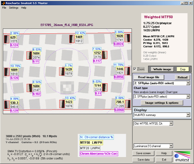
SFRplus results in Rescharts window: Multiple region (ROI) summary
The multi-ROI summary results shown in the Rescharts window (above) is the best summary of SFRplus results. It is described in detail in Multiple ROI (Region of Interest) plot. The upper left contains the image in muted gray tones. The selected regions are surrounded by red rectangles and displayed with full contrast. Four results boxes are displayed next to each region. There is a legend below the image. Distortion statistics are shown in the lower left. SMIA TV distortion is the simplest overall measure of distortion.
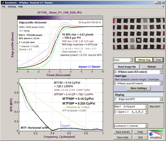
Edge and MTF display in Rescharts window
The Edge and MTF display is identical to the SFR Edge and MTF display. MTF is explained in Sharpness: What is it and how is it measured? The average edge (or line spread function) is plotted on the top and the MTF is plotted on the bottom. There are a number of readouts, including 10-90% rise distance, MTF50, MTF50P (the spatial frequency where MTF is 50% of the peak value; differing from MTF50 only for oversharpened pulses), the secondary readout (MTF20 in this case; selectable to MTFnn or MTFnnP at any contrast level nn or MTF at a spatial frequency specified in cycles/pixel, line pairs/inch or line pairs/mm.), and the MTF at the Nyquist frequency (0.5 cycles/pixel).
Chromatic Aberration
Lateral Chromatic Aberration (LCA), also known as "color
fringing,"
is most visible on tangential boundaries near the edges of the image. Much of the plot is grayed out if the selected region (ROI) is too close to the center (less than 30% of the distance to the corner) to accurately measure CA.
The area between the highest and lowest of the edge curves (shown for the R, G, B, and Y (luminance) channels) is a perceptual measurement of LCA. It has units of pixels because the curves are normalized to an amplitude of 1 and the x-direction (normal to the edge) is in units of pixels. It is displayed as a magenta curve. |
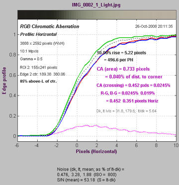
Lateral Chromatic Aberration |
Perceptual LCA is also expressed as percentage of the distance from center to corner, which tends to be more reflective of system performance: less sensitive to location and pixel count than the pixel measurement. Values under 0.04% of the distance from the center are insignificant; LCA over 0.15%
can be quite visible and serious.
Information for correction LCA (R-G and B-G crossing distances) is also given in units of % (center-to-corner) and pixels. LCA can be corrected most effectively before demosaicing. Results are explained in Chromatic Aberration ... plot. |
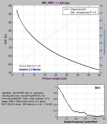
SQF (Subjective Quality Factor)
SQF is a perceptual measurement of the sharpness of a display (monitor image or print). MTF, by comparison is device sharpness (not perceptual sharpness). SQF includes the effects of the human visual system's Contrast Sensitivity Function (CSF), print (or display) size, and viewing distance (which is assumed to be proportional to print height, by default).
See Introduction to SQF for more detail. SQF was developed by Eastman Kodak scientists in 1972. It has been verified and used inside Kodak and Polaroid, but it has remained obscure until now because it was difficult to calculate. Its only significant public exposure has been in Popular Photography lens tests � |
SQF (Subjective Quality Factor) |
Tonal response & gamma
This display is derived from the 4x5 stepchart pattern, located just below the central square of the SFRplus test chart. It resembles the third figure in Stepchart. The upper plot shows the tonal response for all colors. The lower plot shows instantaneous gamma— the slope (derivative) of tonal response. The value of gamma may differ slightly from the values in the Edge response and MTF display because it's calculated differently-- based on the average slope of the light to middle tone squares of the stepchart. |
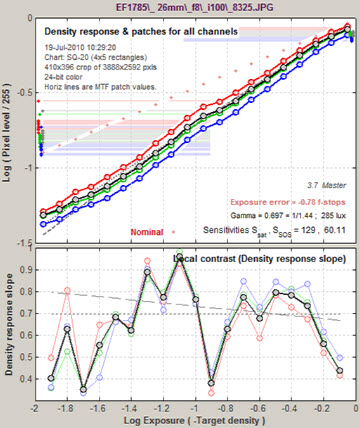
Tonal response & gamma |
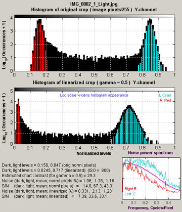
Histograms and noise statistics
This display contains histograms of pixel levels for individual ROIs (original on top and linearized using input gamma on bottom). The black (background) histogram contains pixel levels for the entire ROI. The red histogram is for the light region, away from the transition, used in the noise statistics calculation. The cyan histogram is for the dark region. Sharpening may cause extra bumps to appear in the black histogram.
A detailed signal and noise analyis, described here, is shown below the histograms.
Noise calculations are made in portions of the ROIs (Regions of Interest) away from the transitions. The noise spectrum on the lower right contains qualitative information about noise visibility and software noise reduction, which generally reduces high frequency noise below 0.5, typical of demosaicing alone. The region on the right is shown in red; left is shown in cyan. See also Noise. |
Histograms and noise stats |
Uniformity (Light Falloff)
Measures light falloff (lens vignetting) and sensor uniformity
Imatest™ Uniformity (Light Falloff) measures lens vignetting (dropoff in illumination at the edges of the image) as well as other types of image, illumination, and sensor nonuniformities. Examples include
- the uniformity of flash units (using light bounced off a white wall),
- the uniformity of flatbed scanners,
- sensor noise and spots of the type caused by dust on the sensor (Imatest Master only).
Display options include contours on top of images and pseudocolor with color bar. In Imatest Master , Light Falloff can also display a histogram of pixel levels, analyses of stuck (hot and dead) pixels and color shading, and a detailed image of fine nonuniformities.
Simplified instructions
To prepare an image for Light Falloff, set your camera lens for manual focus and focus it at infinity (the worst case for light falloff). Light Falloff works without a lens if the sensor is evenly illuminated. Photograph an evenly lit subject— a smooth sheet of matte paper (white or gray) is ideal. Get close to the subject, but not so close that you shade it. A diffuser near the lens can be helpful. Outdoors illumination (in the shade) often works best; it's easiest to get even illumination. Getting a uniform image can be a challenge with ultrawide lenses, such as the Canon10-22 mm digital zoom lens at 10mm (equivalent to 16 mm in the 35mm format); it's almost impossible to avoid shading part of the card. For such extreme lenses, a good quality light table with an additional diffuser in front of the lens may be necessary.
The subject does not need to be in focus; the goal is to measure lens light falloff and sensor uniformity, not features of the subject. For typical lens vignetting measurements, set exposure compensation to overexpose by about one f-stop. (You may, however, use any exposure you choose.) More details can be found in the Light Falloff instructions.
Channel contour plot
shows contours of the level (normalized or not) of the selected channel (Red, Green, Blue, or Y (luminance = Y = 0.30*R + 0.59*G + 0.11*B)) of the image file. The contours are superposed on top of the image. In this unnormalized display, the maximum value of 1 corresponds to pixel level = 255 in image files with bit depth = 8. Some lightning nonuniformity is evident in the plot: the top is brighter than the bottom. The contours are derived vrom a smoothed (lowpass filtered) version of the image.
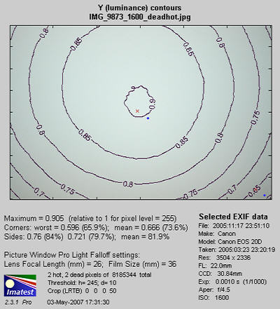
 The text displays the maximum luminance value, the worst and mean corner values (in normalized pixel levels and percentage of maximum), and the side values. Two hot and two dead pixels (which were simulated) were detected with thresholds of 246 and 10 (pixels), respectively. More details of the hot and dead pixels are in the CSV and XML output files. Selected EXIF data is shown on the right.
The setting for correcting light falloff in the Picture Window Pro Light falloff transformation is also given. The PW pro Light Falloff dialog box is shown on the right. Film Size (mm) remains at 36 (the PW Pro default value: the width of a 35mm frame). Picture Window Pro is the powerful and affordable photographic image editor that I use for my own work. The Lens Focal Length is rarely the exact focal length of the lens. Light falloff depends on the lens aperture (f-stop) as well as a number of lens design parameters. Lenses designed designed for digital cameras, where the rays emerging from the rear of the lens remain nearly normal (perpendicular) to the sensor surface, tend to have reduced light falloff.
For aesthetic purposes I generally recommend undercorrecting the image, i.e., using a larger Lens Focal Length. This makes the edges somewhat darker, which is usually pleasing. Ansel Adams routinely burned (darkened) the edges of his prints. Part of the reason was that he had to compensate for light falloff from his enlarger (when he wasn't contact printing).
"My experience indicates that practically every print requires some burning of the edges, especially prints that are to be mounted on a white card, as the flare from the card tends to weaken visually the tonality of the adjacent areas. Edge burning must never be overdone..."
Ansel Adams, "The Print," p. 66. 1966 edition.
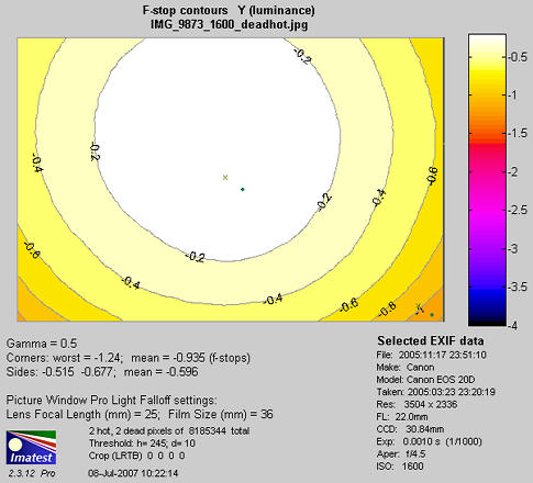
F-stop contour plot
shows contours of the normalized channel levels (R, G, B, or Y) of the image file, measured in f-stops. A pseudocolor display with color bar has been selected. The colors in the color bar are fixed: colors always vary from white at 0 f-stops to black at -4 f-stops and darker. For this plot to be accurate, a good estimate of gamma (the camera's intrinsic contrast) is required. Gamma is measured by Stepchart, using any one of several widely-available step charts. (Reflection charts are easiest to use but transmission charts can also be used to measure dynamic range.)
Gamma can be tricky to measure for several reasons. (1) Many cameras have complex response curves, for example, "S"-curves superposed atop gamma curves. This means that gamma can vary with brightness. (2) Some cameras employ adaptive signal processing in their RAW conversion algorithms. This increases contrast (i.e., gamma) for low contrast subjects and decreases it for contrasty subjects. This improves pictorial quality for a wide range of scenes, but makes measurements difficult, especially since Light falloff targets have the lowest possible contrast.
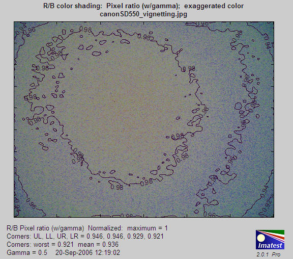
Color shading (nonuniformity) (Imatest Master only)
Light Falloff displays color nonuniformity. This image shows shading measured as the pixel ratio between the red and blue channels, normalized to 1.0 to minimize the effects of white balance errors. The background shows exaggerated colors (HSV saturation S has been increased by 10x for low saturation values; less for high values.) Several display options are available. Details here.
Uniformity profiles (Imatest Master only)
Uniformity profiles, introduced in Imatest Master 2.3.16 (August 2007), displays profiles of image levels along several lines: Diagonal Upper Left-Lower Right, Diagonal Lower Left-Upper Right, Vertical Top-Bottom (center), and Horizontal Left-Right (center). Several display options are available, including unnormalized levels (max 1), pixel levels (max 255), normalized levels (max 2), and R/G and B/G ratios (G constant). Details here. |
 |
Histograms (Imatest Master only)
The histogram plot, introduced in Imatest Master 2.3.11 (July 2007), facilitates the detection and the setting of thresholds for stuck (hot, dead, etc.) pixels. Histograms of log10(occurrences+1) are displayed for the red, green, and blue channels. Details here.
In this example, single stuck pixels are plainly visible near levels 0 and 252. You can quickly see if the thresholds are set correctly— if they are outside the valid density region and if the dead and hot pixels are above and below their respective thresholds. You can change threshold settings and rerun Light Falloff if needed.
Noise detail (Imatest Master only)
shows an exaggerated image of the noise detail, a pseudocolor image of image variation, or a pseudocolor image emphasizing spots.. The algorithm is in the Light Falloff for Imatest Master instructions.
The first image (below) shows noise detail for the Canon EOS-20D at ISO 1600 with the 10-22mm lens set to f/4.5. No surprises here; electronic noise dominates.
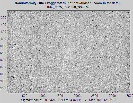
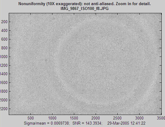
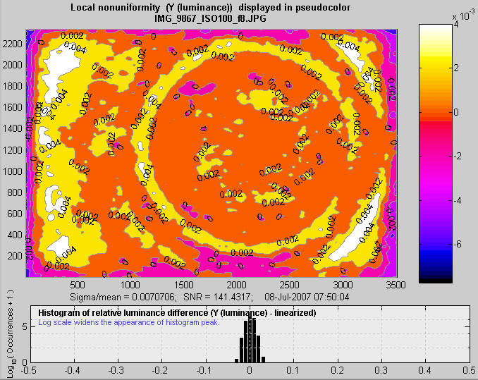
The second image (below) shows noise detail for the Canon EOS-20D at ISO 100 with the 10-22mm lens set to f/8. Thanks to the small aperture, dust spots are visible. The dust is on the anti-aliasing/infrared filter/microlens assembly in front of the sensor. This assembly can be well over 1 millimeter thick. Stopping the lens down (increasing the f-stop setting) reduces the size of dust spots but makes them darker.
This image has a surprise in the form of concentric circles: bands where the noise appears to be higher or lower than the remainder of the image. These bands could be caused caused by the Analog-to-Digital (A-D) converter in the image sensor chip or by JPEG compression. Sensors can have small discontinuities when, for example going from level 127 to 128: binary 01111111 to 10000000. Recall that the nonuniformities are exaggerated by a factor of 10: they would be invisible or barely visible on most images, but you might seem then faintly in smooth areas like skies.
Here is the same image, displayed in pseudocolor (which shows the amount of variation) with a color bar, and including a histogram (of individual pixels, not the smoothed image used to generate the pseudocolor contour plot on the left). This histogram will usually be narrower than the histogram plot shown above because variations at low spatial frequencies have been (lowpass) filtered out.
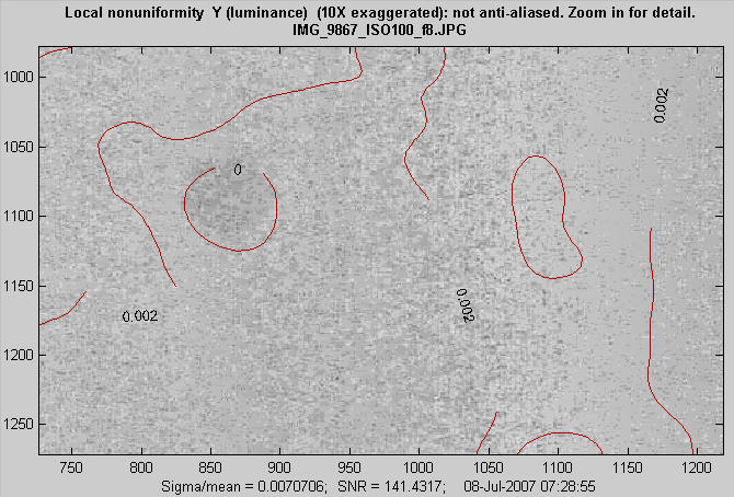
The image below is an enlargement (a zoom) of the above image that includes the dust spot to the left of the center, shown with superposed contours.You can zoom into an image by using the mouse to draw an rectangle, or by simply clicking on a feature you want to enlarge. You can restore the original image by double-clicking anywhere on the image.
Distortion
Measures radial lens distortion
Imatest™ Distortion
- measures radial lens distortion, an aberration that causes straight lines to curve,
- calculates coefficients for removing it, and
- provides additional information on geometric distortions in digital images.
Distortion models assume circular symmetry about a central point, where undistorted and distorted radii ru and rd (distances from the center) are related by equations of the form ru = f( rd ), where f is one of several functions.
In the simplest distortion (third order) model,
ru = rd + k1 rd3.
Because this third-order equation is not adequate for all lenses, Distortion also calculates the coefficients for the fifth-order model,
ru = rd + h1 rd3 + h2 rd5.
Distortion also calculates the coefficients for Picture Window Pro, which uses a tangent/arctangent distortion model,
ru = tan(10 p1 rd )/ (10 p1 ) ; h1 > 0 (barrel distortion)
ru = tan-1(10 p1 rd )/ (10 p1 ) ; h1 < 0 (pincushion distortion)
Distortion has two forms, barrel (k1 > 0) or pincushion (k1 < 0), as illustrated below.
Distortion tends to be most serious in extreme wide angle, telephoto, and zoom lenses. It is most objectionable in architectural photography and photogrammetry — photography used for measurement (metrology). It can be highly visible on tangential lines near the boundaries of the image, but it isn't visible on radial lines. Distortion by Paul van Walree is excellent background reading.
To measure distortion, you'll need a rectangular or (preferably) square grid pattern, which you can create using Test Charts. Print the chart, photograph it (taking care to avoid glare; matte surface recommended), and enter the image into the Imatest Distortion module.
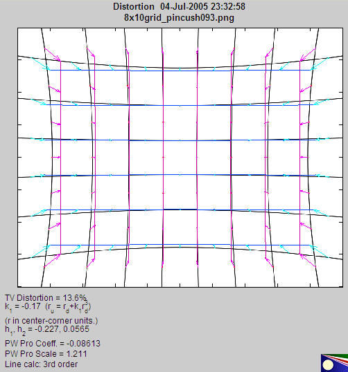
An example of Distortion output is shown below for the Sigma 18-125 mm f/3.5-5.6 DC lens (designed for APS-C-sized sensors, such as the Canon EOS-30D, Digital Rebel, Nikon D100, D70, etc. The Sigma is an excellent lens — a bargain — except for its autofocus. Mine doesn't autofocus as reliably as Canon lenses, but it works beautifully on manual. The autofocus problem is plainly visible when working with the distortion chart.
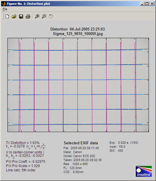
The Sigma has modest amounts of pincushion distortion at 125 mm and barrel distortion at 18mm, its widest angle setting. Results displayed below the image, in the column on the left, include,
 TV Distortion from the SMIA specification, §5.20. Referring to the image on the right,
SMIA TV Distortion = 100( A-B )/B ;
A = ( A1+A2 )/2
The box on the right is described in the SMIA spec as "nearly filling" the image. Since the test chart grid may not do this, Distortion uses a simulated box whose height is 98% that of the image. Note that the sign is opposite of k1.
Although any number in this list can be used as a measure of distortion, SMIA TV distortion may be the best choice because it's the easiest to visualize.
- Coefficient k1 from the third-order equation, ru = rd + k1 rd3 where r is normalized to the center-corner distance. k1 = 0 for no distortion; k1 < 0 for pincushion distortion; k1 > 0 for barrel distortion.
- Coefficients h1 and h1 from the fifth-order equation, ru = rd + h1 rd3 + h2 rd5.
- The Lens Distortion correction coefficient and scale factor for Picture Window Pro. The sign is the same as k1.
Distortion also calculates decentering: the deviation of the center of distortion symmetry from the geometric center of the image. Decentering can result from poor manufacturing quality or mechanical shock (whoops!). Details are in the Distortion instructions.
The plot includes arrows that illustrate the change in radius when distortion is corrected. Distortion was too low on the above plot to make the arrows visible. They are illustrated in the plot below for a large amount of simulated barrel distortion.
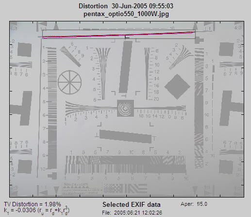
Distortion can also be used with a single line if its curvature is visible. Long tangential lines near the edge of the image are preferred. The ISO 12233 chart contains two such lines, which are adequate but not ideal: they would be better if they were thinner and further from the image center. Here is an example, illustrating a modest amount of pincushion distortion.
In Imatest Master, Distortion can also produce an intersection points figure, showing points where lines cross, and a radius correction figure, showing fine details of the distortion profile.
Print Test
Measures print quality factors: color response, tonal response, and Dmax
Introduction to Print Test
Imatest™ Print Test
measures several of the key factors that contribute to photographic print quality,
- Color response, the relationship between pixels in the image file and colors in the print,
- Color gamut, the range of saturated colors a print can reproduce, i.e., the limits of color response,
- Tonal response, the relation between pixels and print density, and
- Dmax, the deepest printable black tone: a very important image quality factor,
using a simple test pattern scanned on a flatbed scanner. No specialized equipment is required. Print Test can also be used to study the effects of gamut mapping: transformations between different color spaces or devices.
Print quality depends on the
- Printer,
- Paper (manufacturer's or independent),
- Ink (manufacturer's or independent),
- Working color space,
- ICC profile,
- Rendering intent (one of four rules, embedded in ICC profiles, for mapping pixels between color spaces or devices such as monitors and printers
- RIP (Raster Image Processor), optional software packages available as alternatives to standard printer drivers and profiles, and
- Color engine (probably a minor factor); you can choose between Windows ICM 2, Adobe Color Engine (ACE), and Little CMS.
Even if you have only one printer, many options may be available. I use an Epson R2400 printer with standard Ultrachrome inks, but I can choose among a staggering variety of papers and profiles. And the working color space and profile rendering intent can also make a difference.
Print Test can answer questions such as,
- What range of colors can my printer/paper/ink can reproduce, i.e., what is its gamut?
- How dark a black tone can my printer/paper/ink make?
- How good are my ICC profiles? Do they provide smooth, uniform response? Under what conditions do colors saturate? What are their specific strengths and weakness?
- How do colors map between color spaces and devices? What difference does working color space and rendering intent make?
You may, of course, test a new ink/paper/profile combination using one or more test images. Such tests are important, even if you use Print Test. The problem is that one image (say, a landscape) may look fine while another (say, a portrait) may not. The reason lies in details of the tonal and color response revealed by Print test, which can spare you from unpleasant surprises and help you find superior ink/paper/profile combinations.
Although the results are not as accurate in an absolute sense as those produced by expensive spectrophotometers, colorimeters, or densitometers, they are outstanding in a relative sense— for comparing prints made with different printers, inks, papers, working color spaces, and profiles. Absolute accuracy can be quite good in scanners that can be characterized by ICC profiles. The default profile in my Epson 3200 is respectable: its mean color error (ΔE), measured by Colorcheck, is a little over 5; as good as a high quality digital camera. It can be improved by profiling the scanner with one of several available packages (Monaco EZColor, Profile Mechanic - Scanner, etc.). It can be further improved by scanning a Q-13 or equivalent reflective step chart next to the print.
The test pattern, shown on the right, was generated using the HSL color representation.
- H = Hue varies from 0 to 1 for the color range R→ Y→ G→ C→ B→ M→ R (horizontally across the image on the right). (0 to 6 is used in the Figures below for clarity.)
- S = Saturation = max(R,G,B)/min(R,G,B). S = 0 for gray; 1 for the most saturated colors.
- LHSL = Lightness = (max(R,G,B)+min(R,G,B))/2. (The HSL subscript is used to distinguish it from CIELAB L.) L = 0 is pure black; 1 is pure white. The most visually saturated colors occur where LHSL = 0.5.
The key zones are,
- S=1 square. A pattern consisting of all possible hues (0 ≤ H ≤ 1) and lightnesses (0 ≤LHSL≤ 1), where all colors are fully saturated (S = 1), i.e., as saturated as they can be for the lightness value.
- L=0.5 rectangle. A pattern consisting of all possible hues (0 ≤ H ≤ 1) and saturation levels (0 ≤ S ≤ 1) for middle lightness (LHSL = 0.5), where colors are most visually saturated.
- Two identical monochrome tone scales, where pixel levels vary linearly, 0 ≤ {R=G=B}≤ 1.
The zones labelled K, Gry, and W are uniform black (pixel level = 0), gray (pixel level = 127), and white (pixel level = 255), respectively.
Just by looking at the printed test pattern you can see response irregularities with greater detail than with some expensive instruments.
Simplified instructions
Full instructions are found on the Print test instruction page.
- Open one of the Print test patterns located in the images subfolder of the Imatest installation folder. The patterns may also be downloaded by clicking Print_test_target.png, (untagged) or versions tagged with profiles for sRGB, Adobe RGB (1998), and Wide Gamut RGB color spaces. These patterns all contain the same data; only the profile tag differs.
- Print the pattern, approximately 6.5x10 inches (16x25 cm), from your image editor. Carefully record the paper, ink, working color space, ICC profile, rendering intent, and printer software settings.
- Scan the print on a flatbed scanner at around 100 to 150 dpi. (Higher resolution is wasted; it merely slows the calculations.) The pattern must be aligned precisely (not tilted). If possible, the scanner's auto exposure should be turned off and ICC Color Management setting should be used. The output color space should be one of the three recognized by Print test: sRGB (small gamut; comparable to CRTs), Adobe RGB (1998) (larger gamut; comparable to high quality printers), or Wide Gamut RGB (larger gamut than any physical device).Adobe RGB is recommended.
- Save the scan with a descriptive name in TIFF, PNG, or maximum quality JPEG. A reduced scan of a print made on the Epson 2200 printer with Epson Enhanced Matte paper and the standard Epson ICC profile is shown on the right. Colors are somewhat more subdued than glossy or luster surfaces.
- Calibrate. Accuracy is improved if you scan a Q-13 or equivalent reflective step chart next to the print (shown on the right of the above image), then run Q-13 Stepchart. For details, see the Print test instructions.
- Run Imatest. Select the Print test module. Crop the image so a small white border appears around the test pattern. (Be sure to crop out the Q-13 chart in the image on the right.). Select the color spaces used to print and scan the test pattern.
|
Results
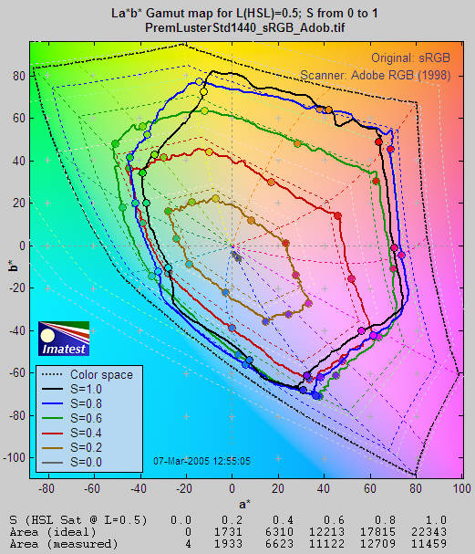
Results below are for Epson 2200 printer with Ultrachrome inks, Premium Luster paper, and the standard 1440 dpi Epson profile.
Density
The first Figure contains the grayscale density response and Dmax, the maximum density of the print, where density is defined as –log10(fraction of reflected light). The value of Dmax (2.24; 0.58% reflectivity) is the average of the upper and right black areas.
The upper plot shows –print density as a function of log10(original pixel level (in the test pattern)/255). This corresponds to a standard density-log exposure characteristic curve for photographic papers. The blue plot is for the upper grayscale; the black plot is for the lower-right grayscale. Somewhat uneven illumination is evident. The print density values are calculated from Q-13 calibration curve (lower right). The thin dashed curves contain –log10(pixel levels).
The lower left curve is the characteristic curve (print vs. original normalized pixel level) on a linear scale.
The lower right curve is the results of the (separate) Q-13 calibration run used to calibrate Dmax and the density plot.
S=1 La*b* Gamut map
The S=1 gamut map displays results for region 1, which contains all possible hues (0 ≤ H ≤ 1) and lightnesses (0 ≤ LHSL ≤ 1) with maximum HSL saturation (S = 1).
The La*b* gamut map uses the device-independent CIELAB color space. In CIELAB, L is a nonlinear function of luminance (where luminance ≈ 0.30*Red + 0.59*Green + 0.11*Blue), a* represents colors ranging from cyan-green to magenta, and b* represents colors from blue to yellow. The colors of the a*b* plane are approximated in the background of the Figure below.
CIELAB is relatively perceptually uniform, meaning that the visible difference between colors is roughly proportional to the distance between them. It isn't perfect, but it's far better than HSL (where Y, C, and M occupy narrow bands) or or the familiar CIE 1931 xyY color space, where gamuts are represented as triangles or hexagons inside a familiar horseshoe curve. A CIE 1931 xyY gamut map proved to be useless because of its perceptual nonuniformity: values bunched up along edges in a way that made results difficult to interpret. Note: The L-values in the box inside the image below refer to LHSL in the test file, not CIELAB L.
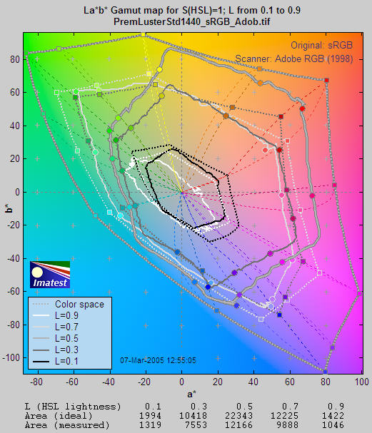
CIELAB color space is often displayed as a solid 3D volume. But although 3D displays can be visually impressive, they can be difficult to interpret. Print test displays an S=1 La*b* Gamut map as cross sections of the La*b* volume representing a*b* values for test file lightnesses (LHSL) of {0.1, 0.3, 0.5, 0.7, and 0.9}, corresponding to near black, dark gray, middle gray, light gray, and near white.
Although this display contains less information than the HSL map (below), but the results are clearer and more useful. The solid shapes from white to black) are the measured response for values of LHSL shown in the legend on the lower left. The dotted shapes represent the gamut of the color space (sRGB, in this case) at each LHSL level. CIELAB gamut varies with lightness: it is largest for middle tones (LHSL = 0.5) and drops to zero for pure white and black. This is closer to the workings of the human eye than HSL representation, where hues vary from 0 to 1, even for white and black.
The dotted concentric curves are the twelve loci of constant hue, representing the six primary hues (R, Y, G, C, B, M) and the six hues halfway between them.. They follow different curves above and below L = 0.5. The circles on the solid curves show the measured hues at locations corresponding to the twelve hue loci. Ideally they should be on the loci. The curves for L = 0.5 (middle gray) are outlined in dark gray to distinguish them from the background.
The hexagonal shape of the gamuts makes it easy to judge performance for each primary. The measured (solid) shape should be compared to the ideal (dotted) shape for each level. Weakness in magenta, blue, and green is very apparent, especially at L = 0.5 and L = 0.7. But the gamut is excellent for L = 0.3.
L=0.5 La*b* Saturation map
The L=0.5 Saturation map is for region 2, which contains all possible hues (0 ≤ H ≤ 1) and saturation levels (0 ≤ S ≤ 1) for middle lightness (LHSL = 0.5), where saturation is highest. This plot,which displays the response to different levels of color saturation, is of interest for comparing different rendering intents (rules that control how colors are mapped when they are transformed between color spaces or color spaces and devices).
Colorimetric rendering intents should leave saturation unchanged unless the output device can't reproduce a color in the color space. Perceptual rendering intent compresses gamut when moving to color spaces with smaller gamut. There is no standard for perceptual rendering intent: every manufacturer does it in their own say. "Perceptual rendering intent" is a vague concept; it's hard to know its precise meaning unless you measure it, which you can do with Print test or with Gamutvision.
Gamuts are shown in the CIELAB a*b* plane for 0 ≤ S ≤ 1 in steps of 0.2. As in the the S=1 La*b* Saturation map, the dotted lines and shapes are the ideal values and the solid shapes are the measured values.
Gamut is excellent for S = 0.2 (brown) and 0.4 (red). But compression becomes apparent around S = 0.4 (red curve) for magenta and blue and S = 0.6 (green curve) for green and cyan, where the printer starts to saturate. Increasing S above these values doesn't increase the print saturation: in fact, saturation decreases slightly at S = 1. This is the result of limitations of the Epson 2200's pigment-based inks and the workings of the standard Epson ICC profile.
With Gamut maps, differences between printers, papers, and profiles are immediately apparent. These differences are far more difficult to visualize without Imatest Print test because each image has its own color gamut. One image may look beautiful but another may be distorted by the printer's limitations.
HSL contour plots
The HSL contour plots below display color response in great detail, but don't contain absolute color information. For that you need the La*b* or CIE 1931 xy plots described above. They work best when the same color space is used to print and scan the target. For these plots to be displayed, Display HSL coutour plots must be checked in the Print test input dialog box.
S=1 HSL Gamut map
The S=1 Figures are for region 1, which contains all possible hues (0 ≤ H ≤ 1) and lightnesses (0 ≤ LHSL ≤ 1) with maximum HSL saturation (S = 1).
The Gamut map shows the print saturation levels for an image that goes from dark to light with maximum saturation. If the print and scanner response were perfect, S would equal 1 everywhere. Weak saturation is evident in light greens and magentas (L > 0.5). Strong saturation in darker regions, roughly 0.2 ≤ L ≤ 0.4, would seem to indicate that a better profile might perform better in the light green and magenta regions. Weak saturation in very light (L>0.95) and dark areas (L<0.1) is not very visible.
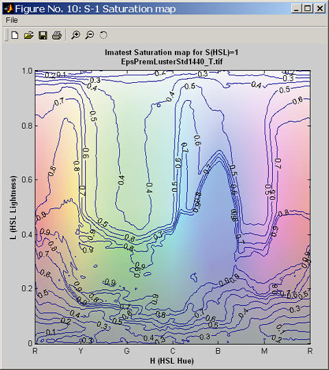
S-1 Lightness and Hue maps are also displayed. They are illustrated in the Print test instructions.
L=0.5 HSL Saturation map
The L=0.5 Figures are for region 2, which contains all possible hues (0 ≤ H ≤ 1) and saturation levels (0 ≤ S ≤ 1) for middle lightness (LHSL = 0.5), where the greatest saturation takes place.
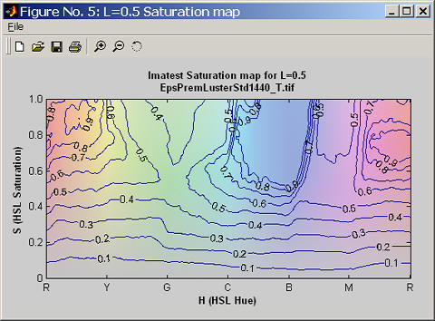
The ideal L=0.5 Saturation map would consist of uniformly spaced horizontal lines from 0.9 to 0.1. The weak saturation in the greens and magentas is visible here. The L*a*b* Saturation map is more generally usefu-- it also shows the weakness in greens and magentas, but in a clearer device-independent format.
An additional Figure with L=0.5 Hue and Lightness maps has been omitted.
Test Charts
Creates test charts for high quality inkjet printers
Imatest™ Test Charts
creates test chart files that can be printed on high quality inkjet printers. A great many options are available. You can select chart type, contrast, highlight color, sine or bar pattern, printer gamma, and more. Bitmap and Scalable Vector Graphics (SVG) charts are available. Charts include
- Bitmap and SVG patterns for use in SFR slanted-edge MTF analysis.
- Star patterns and zone plate, useful for viewing angle-dependent effects and Moiré fringing (colored bands caused by aliasing).
- A log frequency-contrast gradient chart that is useful for viewing Moiré fringing and detail lost to software noise reduction. This loss typically takes place in high spatial frequency/low contrast regions.
- A grid pattern for use with Distortion.
You can either buy test charts or print your own.
Why buy test charts?
- Standardization. You can be confident that your chart is identical to the charts used by others.
- Calibration. Certain charts cannot be properly calibrated when printed on your own printer. These include step charts (the Kodak Q-13/Q-14, etc.) and color charts (the GretagMacbeth Colorchecker, IT-8, etc.). Commercially manufactured charts must be used.
- Resolution. Most commercial charts are printed at higher resolutions than inkjet printers can achieve, and hence may be used at shorter distances— microscopic in some cases. For example, the small Sine Patterns/Applied Image ISO-12233 Resolution Charts (.1X, .5X, and 1X) are printed on photographic paper, which is capable of much finer resolution than inkjet printers. The chart may safely fill the entire frame.
Why print your own?
- Cost. It is much less expensive.
- Convenience. You can use the charts as soon as you print them.
- Quality. Can be excellent with high quality inkjet printers if you photograph them from a sufficient distance.
- Versatility. Many options are available, some of which may not be available on commercial charts. You can use an image editor to modify charts to suit your needs. You can print the chart any size you want: the standard print size is merely a suggestion.
Imatest generates charts that may be impractically large for downloading, but present no problem if generated locally.
Chart patterns
Charts are designed to fit on letter-size (8.5x11 inch), A4, A3, and Super A3/Super B (13x19 inch) paper, but they can be printed any size. A number of options, described below, are available for each chart. The first three patterns, SFR:quadrants, SFR rectangles, and Grid, are available in all versions. The remaining patterns are available in Imatest Master only.
SFR: two rectangles (All versions)
This chart is also used for SFR measurements. It should be cut into two segments (left and right sides) and tilted in a manner similar to the SFR quadrants chart, above, when photographed.
|
 |
Grid (All versions)
Grid generates test charts for the Distortion module. |
|
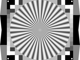
Star chart (Imatest Master only)
Star charts can be used for observing performance (SFR, Moire patterns, and other image processing artifacts) at a variety of angles. In addition to the star (which has a selectable number of bands and either bar or sine form), the chart contains tonal calibration patches and slanted edges for checking results with SFR. Star charts will be analyzed in a future version of Imatest.
|
 |
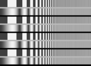
Log frequency-contrast gradient chart (1 and 2-band charts in Imatest Master only)
This chart displays bar or sine patterns of increasing spatial frequency. Several features resemble the Koren 2003 test chart described in Lens testing (pre-Imatest). This chart is valuable for viewing Moire fringing (colored bands caused by aliasing) and detail lost by software noise reduction, which takes place inside the camera and/or RAW converter, and which may remain even if you try to turn it off. Software noise reduction cannot distinguish noise from high spatial frequency low contrast detail, located in the lower right of the 1 and 2-band charts. The two and four band charts are designed to be printed on letter-size or A4 paper and cut into segments to be placed around the target, possibly in different orientations. The Log frequency-contrast chart will be analyzed in the Rescharts module, now under development .
|

1-band chart |
2 and 4-band charts |
Each chart consists of the following patterns in 1, 2, or 4 bands. From top to bottom,
- A bar of increasing spatial frequency (used to determine spatial frequency).
- A sine or bar pattern of increasing spatial frequency (horizontally) and decreasing contrast (vertically) for 1 and 2-band charts. The contrast is proportional to the square of the distance from the bottom of this band. That emphasizes lower contrast areas, where noise reduction causes a loss of detail. It also corresponds to the way the eye sees, i.e., when the pattern contrast is one quarter of its maximum value, it appears to be about half the maximum. The contrast is constant for the 4-band chart, which is available in Imatest Studio.
- (1-band chart only) 20 rectangular patches. 1 and 20 are black (0,0,0), 2 and 19 are middle gray, and 3-18 (16 patches) are a stepchart with density increment of 0.1 (if the chart is printed correctly, i.e., printer gamma mathes the Test Charts setting: some care is required).
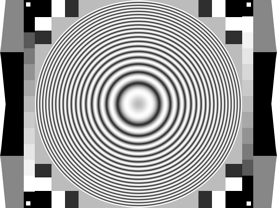
Zone plate (Imatest Master only)
Zone plates (based on Fresnel diffraction) are useful for observing aliasing, particularly Moire patterns and other image processing artifacts. They have a much larger area with high spatial frequencies than the star chart. Thanks to Bart van der Wolf, who has done some interesting work with zone plates. In addition to the zone plate (which has a selectable number of bands and either bar or sine form), the chart contains tonal calibration patches and slanted edges for checking results with SFR.
|
 |
|
Scalable Vector Graphics (SVG) images print at a printer's maximum quality regardless of size. They do not suffer from the pixellation that takes place when bitmap images are enlarged. The SVG chart shown on the right contains squares with slanted edges, "hyperbolic" wedges and bar patterns for viewing moiré caused by aliasing, and a step chart with density steps of 0.1 when the printer is in calibration. Five of these charts printed letter or A4 size and mounted at the center and corners of a 3x3 grid makes an excellent SFR test target, suitable for testing high quality DSLRs. Described here. |
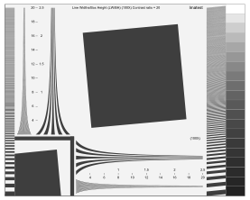 |
Several of the SVG charts consist of slanted squares arranaged on an m x n grid. A step chart (density increment = 0.1) and a pair of hyperbolic wedges may be optionally added. The chart's contrast, brightness, and several other details are adjustable. A typical SVG SFR chart, consisting of a 5x9 grid, is shown below. This chart is optimized to be printed large: on 24 inch widebody printers. It offers significant advantages over standard ISO 12233 charts: less wasted area, better suited to automated testing, larger ROI location tolerance, and better contrast control. These advantages are discussed here.
SVG SFR chart: 5x9 grid, 20:1 contrast, with optional hyperbolic wedge
and step patterns (0.1 density increment) .
Options
A number of options are available, including
 Pixels per inch (PPI) for printing the chart. Affects the pixel size of the chart file.
 - Chart height (cm) . Choose from 18 cm (for A4), 20 cm (for US letter; 8.5x11 in.), 28 cm (for A3), or 30 cm (for Super A3/Super B; 13x19 in.). The chart can be printed any size. The number of vertical pixels is PPI * Chart height (cm) / 2.54.
- Highlight color. In addition to the standard White/Black (or White/Gray) charts, you can replace white with any additive or subtractive primary color: R, G, B, C, M, or Y. Bayer sensors, used in most digital cameras, have half as many R and B sensors as G. Patterns with different highlight colors may perform differently in sharpness tests. A magenta star pattern is illustrated on the right.
- Chart lightness. Affects the highlight color in charts with grayscale images (Star, Log-frequency, Zone plate). Lightest uses the least ink, but response may be smoother when one of the darker values is chosen.
- Type (bar or sine). A bar star pattern is shown on the right; a sine star pattern is illustrated above.
- Star pattern bands. Multiples of 4. The magenta pattern (on the right) has 36 bands); the above White-Black pattern above has 20 bands.
- Contrast ratio. The ratio of the reflectivity of the light to dark areas (the upper zone only in the Log frequency chart). The maximum contrast ratio depends on the printer and paper. It is typically 100 or more for glossy (or luster) surfaces, but only around 60 for matte surfaces. Maximum print density = -log10(minimum reflectivity) can be measured in Print Test. Reducing contrast ratio reduces clipping, which can be a problem in SFR measurements. The default value is 40 (the minimum recommended by the ISO standard), but 20 is recommended in most cases.
- Gamma. You should use the value of gamma for your typical color space and workflow (2.2 is standard for Windows; 1.8 for older Mac systems). The default value of 2.0 is close enough to both for most purposes. Gamma affects the accuracy of grayscale patterns and the actual printed contrast ratio: it must be accurate to get the correct ratio.
- Ink spread compensation corrects for ink spread (or "dot gain") in the Log frequency chart. Others may be added later.) The default is 0. The best value must be determined experimentally.
Multicharts
Interactive analysis of several test charts
Introduction to Multicharts:
measure color accuracy and tonal response
Imatest™ Multicharts analyzes images of color test charts for tonal response and color accuracy using a highly interactive user interface. It can be used to measure white balance and color response in a wide range of lighting conditions and scenes. It can also display the tonal response of monochrome charts and calculate a color correction matrix (Imatest Master only). Multicharts currently supports
You can select either standard chart reference values or you can read in values from data files (Imatest Master only). Values for the two ColorCheckers have been supplied courtesy of X-Rite. You can select between six image file color spaces: sRGB, Adobe RGB (1998), Wide Gamut RGB, ProPhoto RGB, Apple RGB, or ColorMatch. Danny Pascale/Babelcolor's page on the ColorChecker contains nearly everything you want to know about the chart. Ian Lyons has a nice description of IT8.7 charts.
Before running Multicharts, photograph the chart, taking care to avoid glare. For testing white balance, you can photograph the chart in a scene (the mini ColorChecker is especially suitable). Then click on Multicharts in the main Imatest window. To load the image file, click the appropriate chart type in the box below Read image file. Chart type: Crop it, then enter any needed data in the input dialog box.
Differences between Colorcheck and Multicharts
- Multicharts can analyze the IT8.7, CMP DT003, QPcard, and ColorChecker SG charts (SG in Pro only) in addition to the 24-patch Colorchecker.
- Multicharts is highly interactive. You can choose among a large number of displays and options after the the chart image has been entered.
- Multicharts does not currently perform a noise range analysis.
|
Example: the 24-patch ColorChecker, shown with the 2D a*b* plot
The left image shows the 2D a*b* display. Ideal (square) and camera (circle) {a*, b*} patch values are shown. The Chart view box allows you to select among several displays.. |
|
The upper right image shows the color chart. One of several displays can be selected with the buttons just below the image: Ideal the ideal image (as is; unmapped), Id>M the ideal image mapped to sRGB color space (which is close to most monitor displays), Input the input (camera) image unmapped, and In>M the input (camera) image mapped to sRGB. |
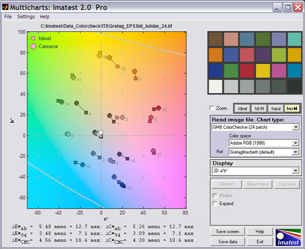
2D a*b * display for ColorChecker
The lower left region shows color differences, using several different metrics. |
|
The lower right region is the display control and option area. |
The available displays, selected by the Display box, include
- Pseudocolor color difference. Shows the difference between the ideal and input color patches using any of several metrics. Probe is available for this display.
- 3D color difference.
- Split colors: ideal/input. Shows the patches split so that the ideal and input values are displayed in the upper left and the lower right or each patch region, respectively. Probe is available for this display.
- xy chromaticity.
- u'v' chromaticity.
- Black & White density.
- 3D L*a*b*. Shown on the right. L*a*b* coordinates can be difficult to visualize when viewed from a single angle. It can be rotated (automatically by pressing the A-rotate button) for improved visualization.
- EXIF data and Color matrix. Shows EXIF data if available and the color correction matrix if it has been calculated.
|
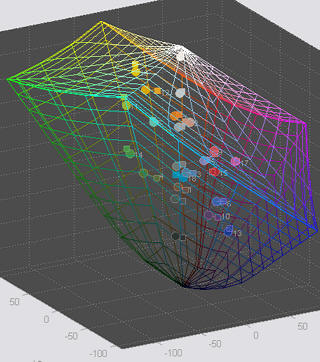 3D L*a*b* display for ColorChecker
 |
Examples of different charts and displays
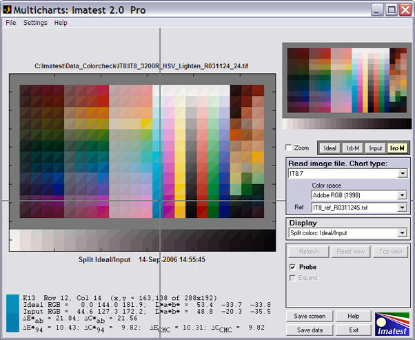
Split display for IT8.7
This Multicharts split display is shown above for a reflective IT8.7 chart, with the Probe turned on. In each patch, the upper left portion is the ideal (reference) value, converted to sRGB for screen display, while the lower right is the input value, also converted to sRGB for screen display. The image is synthesized.
The Probe has been turned on by checking the Probe box on the right. When the probe is on, you can probe any patch in either image. The probe data (for the individual patch), shown below the split display, includes an image of the ideal and input patch colors, ideal and input RGB and L*a*b* values, and several ΔE* and ΔC* color difference metrics. ΔE*ab, the geometric distance in L*a*b* space, is the most familiar, but ΔE*94, which is lower for saturation differences in saturated colors, may be a better measure of visual color difference. It's easy to correlate ΔE* metrics with visual color differences using this display. None of the metrics are perfect! The probe is turned off by clicking outside the images.
The pseudocolor display is shown on the right. Differences can be displayed for several color metrics: ΔE*ab, ΔC*ab, ΔE*94, ΔC*94, ΔE*CMC, ΔC*CMC, ΔL*, ΔChroma, Δ|Hue distance| , Δ(Hue angle) , Chroma (input) and Chroma (output). Several color maps are available. |
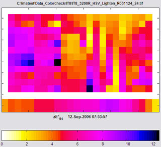 Pseudocolor display for IT8.7
 |
IT8.7 charts are printed on photographic paper. They must be used with reference files. Here are a few sources: Monaco IT8 reference files | Kodak Q60 targets (FTP site) | Wolf Faust (Coloraid.de)
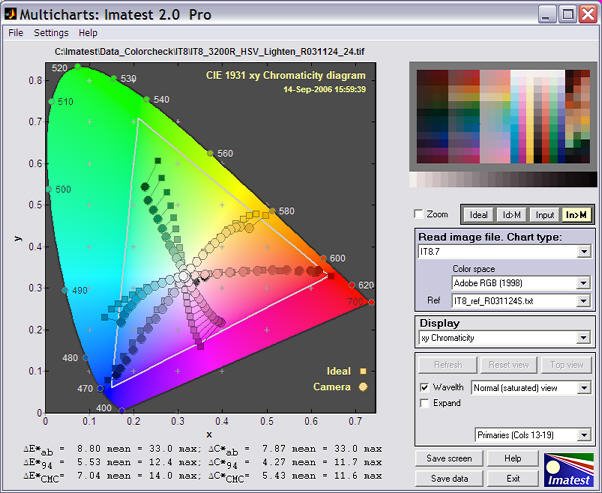
xy Chromaticity display for IT8.7
The xy Chromaticity diagram for the IT8.7 chart is of special interest. To avoid clutter it doesn't display all the patches (this is also the case for the ColorChecker SG and the CMP DC003). Instead it displays values for one of five zones in the chart: columns 13-19 (primaries), 1-4 (dark), 5-8 (mid), 9-12 (dark), and 20-22 (miscellaneous— different for different manufacturer's charts). The primary region (columns 13-19, shown above) is the most interesting since it shows the response to the subtractive and additive primaries, and gives some indication (though far from perfect) of the color gamut of the device + color space under measurement.
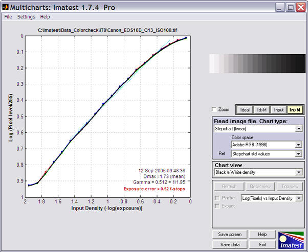
B&W plot: Log(Pixels) vs. Input density for Q-13
The final example of the tour shows the grayscale response curve, in this case Log10(Pixel level) vs. Input density. Gamma is the average slope of this curve for the lighter regions. This plot is also available for all of the color charts because all of them contain grayscale regions. Several additional B&W curves are available.
| Log(pixels vs. input density) |
The slope in the region where input density is between about 0.1 and 1.0 is gamma. Curves for the R, G, and B channels are shown in addition to Luminance. |
| Output vs. input density |
The slope is ideally 1. Density is proportional to -Log10(Luminance). |
| Output vs. input luminance |
Shown on a linear scale. |
| Output vs. input L* a* b* c* |
Uses CIELAB values instead of density or (linear) luminance. Includes color values: 10x a* (green-red), b* (blue -yellow), and c* (chrominance: (a*2 + b*2 )1/2 ). |
GretagMacbethTM and ColorChecker® are trademarks of X-Rite, Incorporated, which is not affiliated with Imatest. ColorChecker L*a*b* values are supplied courtesy of X-Rite.
Rescharts
Analysis of resolution-related charts
Introduction
Imatest™ Rescharts analyzes images of several test charts for resolution-related parameters such as sharpness (i.e., spatial frequency response; MTF), color moiré, and fine detail lost to software noise reduction, using a highly interactive user interface is similar to Multicharts.
The following chart types are supported by Rescharts.
Duplicates SFR, but with a far more interactive interface. It calculates and displays the average edge, SFR (Spatial Frequency Response or MTF), and Lateral Chromatic Aberration. Includes one figure not in SFR: a histogram with noise analysis.
It supports all charts that contain slanted edge patterns, including the ISO 12233 chart and its derivatives. Charts may be purchased from sources such as Applied Image or created with Test Charts (SVG charts are especially recommended) and printed on a high quality inkjet.
|
|
SFRplus
Highly automated analysis of SFR (MTF), Lateral Chromatic Aberration, distortion, and tonal response. Introduced in Imatest 3.2. Uses a special test chart, shown on the left. Unlike other Rescharts modules, SFRplus does not require manual region (ROI) selection: it is performed automatically. Running SFRplus in Rescharts saves settings for fully automated runs.
SFRplus instructions |
|
|
Log Frequency (simple)
Analyzes a sine or bar pattern of increasing spatial frequency. Measures SFR more directly, but less precisely, than the slanted-edge method. Also measures color moiré (Imatest Master only), which is a function of lens sharpness, anti-aliasing filter, and demosaicing algorithm. Spatial frequencies are detected automatically. Charts can be created by Test Charts and printed on a high quality inkjet printer. Also works with the old test chart in Lens testing.
Log Frequency instructions |
|
|
Log F-Contrast (Imatest Master only)
Analyzes a sine or bar pattern of increasing spatial frequency on the one axis and decreasing contrast on the other. Measures SFR for a range of contrast levels. Useful for measuring the loss of fine detail caused by software noise reduction— the effects of nonlinear signal processing. The chart can be created by Test Charts and printed on a high quality inkjet printer.
Log F-Contrast instructions |
|
|
Star chart (Imatest Master only)
Analyzes a sinusoidally-modulated Siemens star chart (144, 72, or 48 cycles); proposed for the revised ISO 12233 standard. Measures MTF (SFR) for 8, 12, or 24 segments around the circle. Has a large variety of displays. The chart can be purchased from Image Engineering or created by Test Charts and printed on a high quality inkjet printer.
Star Chart instructions |
Getting started
Instructions for purchasing or creating test charts can be found on pages for individual tests: SFR, Log Frequency, and Log F-Contrast.
Photograph or scan the chart, taking care to avoid glare, which can be problematic in charts with semigloss and glossy surfaces. Glare can be especially difficult to control with wide angle lenses. A recommended lighting setup is described here and in How to build a testing lab.
To start Rescharts, run Imatest, then click the Rescharts button. The Rescharts window will appear with brief instructions, which may be more up-to-date than the ones shown below.
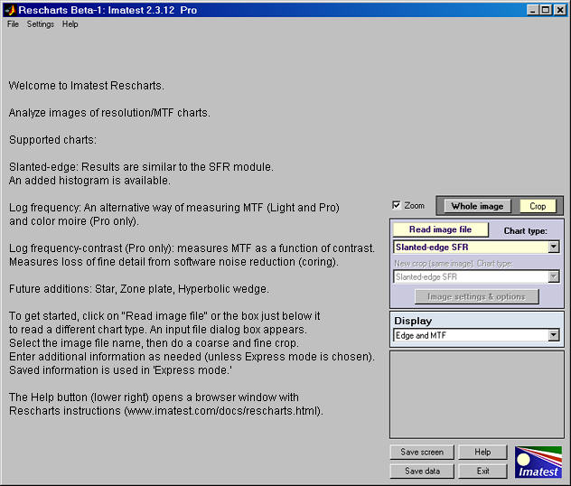
Select an image to analyze by
- clicking on Read image file if the correct Chart type is displayed, or by
- clicking on one of the entries in the popup menu below Chart type:.
The Read image file button and Chart type popup menu are highlighted (yellow background) when Rescharts starts. |
 |
A standard Windows dialog appears with the chart type indicated in the title. Open the image file. Multiple files can be opened for averaging (but batch (sequential) runs are not supported by Rescharts).
If the folder contains meaningless camera-generated file names such as IMG_3734.jpg, IMG_3735.jpg, etc., you can change them to meaningful names that include focal length, aperture, etc., with the View/Rename Files utility, which takes advantage of EXIF data stored in each file.
For all modules other than SFRplus, if the image is the same size and type as the previous image analyzed by Rescharts, you'll be asked if you want to use the same ROI (region of interest). (ROI selection is entirely automatic with SFRplus.)
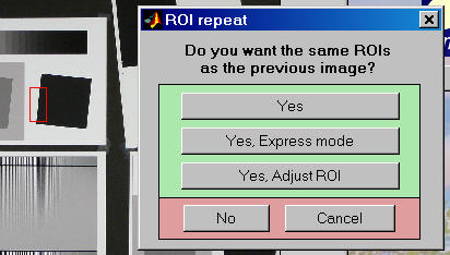
If the image size or type is different or if you answer No, a coarse cropping box appears. The initial crop doesn't have to be precise: you'll have a chance to refine it.
- For Slanted-Edge SFR, select the region you want. Recommended cropping.
- For Log Frequency (simple), select a narrow strip running from along the direction of increasing spatial frequency. Narrow strips of the Log Frequency-Contrast chart can be used.
- For Log F-Contrast, select most of the chart image, leaving small margins (1/2 to 1% of the image dimensions) at the edges.
After the rough crop has been selected, the fine adjustment box appears, showing the coarse crop as a rectangle. This dialog box can be enlarged or maximized to facilitate the adjustment. It offers numerous options.
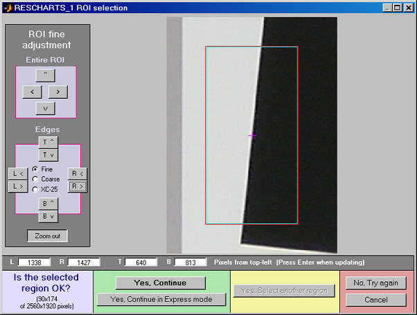
Crop for the Log Frequency-contrast chart. Leave a small margin
(1/2 - 1% of the image height) at the top and bottom.
- The entire ROI can be moved ( ^ > v < , upper-left).
- The top, bottom, left, or right sides can be moved ( T^ Tv R> R< B^ Bv L> L< , middle-left).
- You can choose between Fine, Coarse, and Extra Coarse movement (1, 5, or 25 pixels of movement per click).
- The display can be zoomed out or in.
- Pixel values for the four corners can be entered (X(tl), Y(br), ..., where tl = top-left, br = bottom right, etc.). The origin is the upper-left. Be sure to press the Enter key after entering a value.
When you have completed the fine adjustment, click one of the buttons on the bottom of the window. If you click Yes, Continue , an additional dialog box may appear. The entries in this dialog box can be changed later by clicking on Image settings & options in the Rescharts window. If you click Yes, Continue in Express mode , it will go directly to the Rescharts window, using saved (recent) values.
The Rescharts window
After the image file has been entered, calculations are performed and the most recent Chart view is displayed. The MTF/contrast (2D pseudocolor contour) display (actual MTF when a sine chart is used) for Log F-Contrast is shown below.
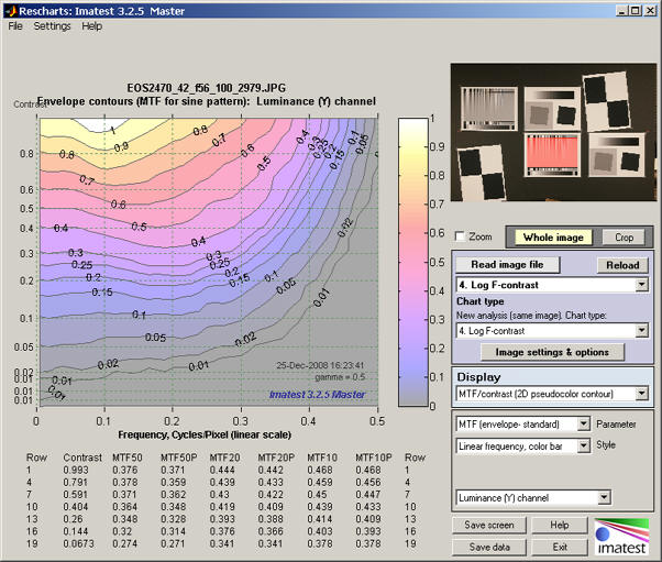
MTF contours for Canon EOS-20D, 24-70mm f/2.8L, 42mm, f/5.6, ISO 100
The main display image is on the upper left. Additional text results may appear below this image. An image of the chart is shown on the upper right. You can choose to display the whole image or the crop (ROI). The remainder of the right side is the control area.
The Zoom checkbox turns Zoom on and off.
The buttons to the right of Zoom set the display to either the Whole image or a Crop of the image (the selected ROI).
Image and Display areas
The image area is on the right of the Rescharts window, just below the Whole image and Crop buttons. It includes the the Read image file and Reload buttons, the Chart type dropdown menu (described above), and additional controls.
Reload reloads an image from a file or reacquires it from a device or video stream (depending on how the image was originally acquired). It is most valuable for versions of Imatest that can acquire images from devices or streams.
Immediately below the Chart type menu is the New crop (same image) menu, which has identical entries. If an item is selected on this menu, the image is recropped for analysis by the selected chart type (which may be the same or different). This menu is useful when several regions of an image need to be analyzed or when the target contains more than one chart type.
Image settings & options brings up the input dialog box for the selected chart type. This is the same box that appears when you press Yes, continue (not Express mode) in the ROI repeat or ROI selection window.
Display, immediately below the image area, selects the results to display. Choices depend on the chart type.
|
|
The Display options area is immediately below Display. The contents, which depend on the Display selection, are described below in the sections for the individual displays.
Save screen (shown on the right) saves a snapshot of the current display (the entire Rescharts screen) as a PNG file (a widely-used losslessly-compressed format). It also allows you to immediately view the snapshot (if the Open window... box is checked) so it can be used a reference for comparing with other results.
File name and Directory at the top of the window set the location of the file to save.
When you check the Open window in an image viewer... box, the current screen will be opened either the system default viewer (if the box under Image viewer is blank) or a viewer/editor of your choice (if the box contains the path name to the viewer/editor). I recommend Irfanview, which is fast, compact, free, and supports an amazing number of image file formats. (It can be valuable for converting nonstandard images to Imatest-readable formats.) Its normal location in English language installations is C:\Program Files\IrfanView\i_view32.exe. |
 |
Save data Saves detailed results in CSV and XML formats. The exact content depends on the module.
Help opens this web page in an HTML browser window.
Exit terminates Imatest Rescharts, but the Imatest main window remains available.
Rescharts modules
This section describes the Rescharts modules, illustrating some of the available displays and options. More information is available in the pages for the individual modules (Chart type analyses).
Slanted-edge SFR
Slanted-edge SFR measures sharpness as Spatial Frequency Response, also called MTF (Modulation Transfer Function) from images of slanted edges, as described in Sharpness. ROI (Region of Interest) selection, calculations, and output largely duplicate SFR. Available displays:
| Edge and MTF (shown on the right) |
| Chromatic Aberration (right, below) |
| SQF (Subjective Quality Factor) |
| Noise spectrum & Shannon capacity |
| Histograms & noise stats (left, below) |
| Summary & EXIF (for JPEGs) |
The principal differences from SFR are the highly interactive interface and an added histogram of the ROI levels, shown below. Black is the entire ROI. Cyan is the portion on the left and red is the portion on the right, both away from the edge. The upper histogram is for the original image (pixel levels/255); the lower histogram is for the linearized image (gamma applied). |
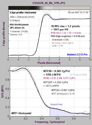
SFR Edge and MTF display
|
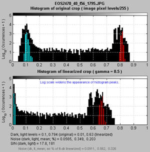
SFR Histogram |
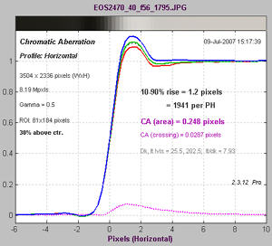
SFR Lateral Chromatic Aberration |
SFRplus
| SFRplus, introduced in Imatest 3.2, performs a highly automated analysis of SFR (MTF), lateral chromatic aberration, distortion, and tonal response, using a special test chart. Unlike other Rescharts modules, SFRplus does not require manual region (ROI) selection: it is performed automatically. Running SFRplus in Rescharts saves settings for fully automated runs. |
| Edge and MTF |
| Chromatic Aberration |
| SQF |
| Noise spectrum & Shannon capacity |
| Multi-ROI summary |
| Tonal response & gamma |
| Histograms and noise stats |
| Summary & EXIF (for JPEGs) |
|
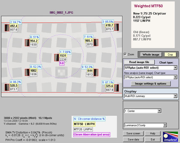
SFRplus summary display for 9 automatically-selected regions
Log Frequency (simple)

Log frequency image: right-click to download an image that can be used for testing.
Log Frequency measures image contrast of charts that increase in spatial frequency on a logarithmic scale (log frequency increases with x). When the image pattern is sinusoidal (not a bar pattern) the contrast is equivalent to SFR or MTF. This method is more direct than Slanted-edge SFR, but less accurate because it is degraded by noise and sampling phase variation. It also measures color moiré (Imatest Master only). The chart can be created by Test Charts and printed on a high quality inkjet. Also works with the test chart in Lens testing and narrow strips of the Log Frequency-Contrast chart..
Available displays: Full instructions
| The Pattern (original pixel levels and linearized) |
| MTF and Moire (linear frequency scale) |
| MTF and Moire (log frequency scale) |
| EXIF data |
The display on the right shows Contrast (MTF) on the top and color moire on the bottom as a function of spatial frequency (displayed linearly). Color moire can me measured in several ways: R-B (normalized Red − Blue channel) is shown on the right. The total color moire is the spread of values above 0.3 cycles/pixels (indicated by the red curve). Details of the color moire measurement can be found in Log Frequency. The Correct for color density box should be checked for best results.
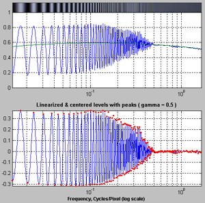
Pattern (original pixel levels and linearized)
|
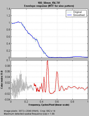
Log Frequency MTF and moire display
(linear x-axis frequency scale) |
Log F-Contrast
Log F-Contrast (short for Log Frequency-Contrast) measures the image contrast of charts that vary in spatial frequency on one axis (log frequency increases with x) and in contrast on the other (contrast is proportional to ( y/h)2 for image height h). When the image pattern is sinusoidal (rather than a bar pattern) the contrast is equivalent to SFR or MTF. This module can be used to measure how much fine, low-contrast detail is lost to software noise reduction. The chart can be created by Test Charts and printed on a high quality inkjet printer.
Available displays: Full instructions
| The Pattern (original pixel levels and linearized) |
| MTF (linear frequency scale) |
| MTF (log frequency scale) |
|
2D pseudocolor contour plots that can display any of several MTF-related parameters: |
MTF (envelope - standard) (standard MTF, normalized to 1 at maximum contrast and zero spatial frequency) |
Normalized contrast level (MTF normalized to 1 at zero spatial frequency for all contrast levels) |
Normalized contrast loss (MTF normalized to 1 at zero spatial frequency for all contrast levels as well as all spatial frequencies at the maximum contrast level: shows contrast loss from ideal) |
| MTFnn or MTFnnP (spatial frequencies where MTF = nn% of the low frequency or peak value |
| EXIF data |
The displays on the right show the Normalized contrast level (MTF normalized to 1 at low spatial frequencies for all chart contrast levels) for the Panasonic TZ1 camera with ISO speed set at 80 (top) and 800 (bottom). Spatial frequency is on a linear scale with a maximum displayed frequency of 0.5 cycles/pixel. The difference between the two images is quite striking. The TZ1 has much more noise reduction— and correspondingly less detail— at ISO 800. These plots are explained in detail in Log F-contrast. |
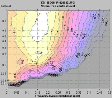
Normalized contrast level (MTF)
(1 at low frequencies
for all chart contrasts):
Panasonic TZ1, ISO 80
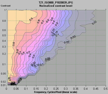
Normalized contrast level: TZ1, ISO 800 |
Star chart
Star Chart measures contrast (MTF or SFR) of sinusoidally-modulated star charts (also known as the Siemens star) proposed for inclusion in the updated ISO 12233 standard. Charts have 144, 72, or 48 cycles and can be analyzed in 8, 12, or 24 segments. Star charts can be purchased from Image Engineering or created by Test Charts and printed on a high quality inkjet printer.
Available displays: Full instructions
| Display |
Description |
| MTF (original and linearized) |
MTF for up to 8 segments of the star. Both linear and logarithmic frequency displays are available. |
| MTFnn or MTFnnP |
Display MTFnn (the frequencies where MTF equals nn % of the low frequency values) and MTFnnP (the frequencies where MTF equals nn % of the peak value) for nn = 70, 50, 30, 20, and 10. Both polar (spider) and rectangular plots are available. |
| MTF contours (rectangular) |
Display MTF contours in a rectangular plot with linear or logarithmic frequency display. Similar to the MTFnn rectangular plot. |
| MTF contours (polar) |
Display MTF contours in a polar plot whose geometry duplicates that of the target. |
| EXIF data |
Show EXIF data if available. |
The displays on the right show MTF contours and MTF70 through MTF10 (spatial frequencies where MTF = 70 through 10% of the low frequency level). Spatial frequency is displayed in cycles per pixel, but Line Widths per Picture Height (LW/PH), cycles/inch, or cycles/mm can be selected by pressing Image settings & options. |
MTF contours, rectangular display,
Linear frequency scale.
MTF70 – MTF10: Polar coordinates,
Linear frequency on radius. |
Imatest IT
Executable programs for automated testing
Introduction
Imatest™ API* is a set of modules designed to
measure image quality in automated testing systems.
Their tight integration with Imatest Master makes it easy to
get them up and running quickly.
*API is an acronym for Application program interface.
With Imatest API you can use the same mathematical engine
to measure image quality on the manufacturing floor
that you used in the development lab. |
The initial API release (April 2007) is a set of EXE (Windows executable) programs, called API/EXE, which includes the following modules:
| Module (with
link to instructions) |
| SFR.exe |
measures sharpness (MTF) using slanted edges of nearly any angle. Multiple regions may be selected in an image. |
| Colorcheck.exe |
measures color accuracy and white balance using the GretagMacbeth Colorchecker (24 patches). |
| Distortion.exe |
measures lens distortion (pincushion or barrel) using a grid pattern. |
| Stepchart.exe |
measures tonal response and dynamic range. |
| Uniformity.exe |
(Light Falloff) measures illumination nonuniformity caused by lens vignetting, etc. |
|
How Imatest API/EXE works
Imatest API/EXE is a set of standalone programs initiated by DOS calls from the test system. They have the same functionality as the corresponding modules in Imatest Master, but they operate without user intervention, making them suitable for use in automated systems. API/EXE modules are represented by the blue box in the figure on the right. The test system interacts with the API/EXE programs through files specified in the DOS command line: the primary inputs are an image file and an INI control file (created and saved by Imatest Master during setup). The output is data files in XML or Excel-readable .CSV format. Figures can be saved if desired.
Although Imatest API/EXE operates independently of Imatest Master, we strongly recommend that API/EXE users have at least one Imatest Master installation on site.
See Imatest API/EXE instructions for detailed instructions for all modules.
Licensing
The license allows you one computer installation (one station) per module. Contact us to discuss quantity discounts. Purchasers should be familiar with the installation and operation of Imatest Master, which is necessary for setting up EXE runs. The license includes a reasonable amount of support (up to three hours) to get you up and running.
Contact
 to purchase an API/EXE modules or to request a free 30 day time-limited trial. We can issue Paypal invoices, and we can accept payments by several means, including wire transfer. (We are developing a more automated purchase/download system.)
Imatest API will not be available for public download. When we receive your request for a 30 day trial, your payment, or approve your purchase order, we will either send you instructions for downloading the installation files or send you the files themselves (typically around 800 kB per module). Contact us to discuss delivery details.
More about Imatest API
Imatest plans to introduce API/DLL programs about two months after the introduction of API/EXE in April 2007. API/DLL will be priced slightly higher than API/EXE. API/EXE users will be able to upgrade for the price difference. Many API/DLL installations will require some customization and support. Feel free to contact us with your specific requirements.
We also plan to introduce new test charts (using scalable vector graphics) along with modifications of sfr.exe that will support automatic region of interest (ROI) selection. This will allow for more framing tolerance in MTF tests.
Imatest API/EXE instructions
Image Quality
Image quality factors
Overview and Imatest measurements
Image quality is one of those concepts that is greater than the sum of its parts. But you can't ignore the parts if your goal is to produce images of the highest quality. Every image quality factor counts.
This page introduces the key image quality factors, describes how Imatest™ measures them, and explains what, if anything, can be done to improve them. It is a guide to Imatest organized by image quality factor. Other guides include the Tour (organized by module) and Imatest documentation (the Table of Contents).
To illustrate the quality factors, we use this early morning image of Monument Valley from Hunt's Mesa, near the Arizona-Utah border. A 13x19 print (available for purchase) is breathtaking, though it can't capture the experience of grabbing the camera gear and running for the truck as the storm broke. Hunt's Mesa isn't public land; you need a Navajo guide to get there. Tom Phillips does an excellent job.
The image was extensively edited. The unedited image, straight from the RAW converter (with some tonal adjustment) is shown below.
When people ask me about "digital manipulation" I delight in telling them that I would no more manipulate an image than Ansel Adams. Of course I'm jesting. In Ansel Adams: A Biography, Mary Street Alinder describes how Adams printed his famous Moonrise over Hernandez image. He'd spend the entire morning making test prints — dodging, burning, and (chemically) manipulating them until they met his exacting standards. It took him that long even though he kept meticulous notes. Then he'd spend the afternoon making prints. From a processing viewpoint he would have loved digital. But probably not from a business viewpoint. Thanks in part to his brilliant business manager he earned more in an afternoon of printing than most of us earn in a decade.
There are two key aspects of image quality.
- Factors affected by post-processing. Contrast, color balance, color saturation, etc. These are the factors that can be enhanced in the darkroom — digital or chemical — under the control of you, the photographer. For example, higher contrast images usually score higher in visual quality assessment tests, unless the image is clipped. Because of their great importance to photo finishers these factors are the focus of much image quality literature. But they're outside the scope of Imatest.
- Factors intrinsic to cameras, lenses, and printers. Sharpness, noise, dynamic range, color accuracy, color gamut, etc. Imatest focuses on these. Imatest modules are summarized on the right.
|
 |
Summary table
This table summarizes the image quality factors described in detail below.
| Quality factor |
Chart |
Module |
Comments |
Camera, lens |
| Color accuracy |
GretagMacbeth ColorChecker (24-patch) |
Colorcheck, Multicharts |
|
| IT8.7 |
Multicharts |
|
| ColorChecker SG |
Multicharts |
Imatest Master only |
| Custom "pie" charts |
Multicharts |
Imatest Master only |
| Dynamic range, Tonal response, Contrast |
Step charts |
Stepchart |
Transmission charts such as the Stouffer T4110 recommended for DR. Algorithm |
| Reflective step charts |
Dynamic Range |
More convenient for measuring DR than Stepchart because it doesn't require a transmission chart. |
| Special charts: ISO-16067-1, QA-62, EIA Grayscale, ISO-14524
OECF, ISO-15739
Noise |
Stepchart |
Imatest Master only. Most are available from Applied Image. |
| ColorChecker, ColorChecker SG, IT8.7, Step Charts |
Multicharts |
|
| SFRplus |
SFRplus |
Does not measure DR. Highly automated. Measures several factors. |
| Exposure accuracy |
Step chart (reflective) |
Stepchart |
|
| GretagMacbeth ColorChecker |
Colorcheck |
|
| Lateral chromatic aberration |
Slanted edge |
SFR |
Printable by Test Charts |
| ISO 12233, Applied Image QA-77 |
Printed on photographic media |
| Lens distortion |
Square or rectangular grid or checkerboard, |
Distortion |
Printable by Test Charts or displayed on LDC flat screen monitor with Screen Patterns. |
| SFRplus |
SFRplus |
Highly automated. Measures several factors. |
| Light falloff, vignetting |
plain, uniformly lit surface |
Lightfall |
Can be displayed on LDC flat screen monitor with Screen Patterns. |
| Noise |
Step charts |
Stepchart |
|
| GretagMacbeth ColorChecker |
Colorcheck |
|
| Sharpness (MTF) |
Slanted-edge |
SFR |
Printable by Test Charts Algorithm |
| ISO 12233, Applied Image QA-77 |
Printed on photographic media |
| SFRplus |
SFRplus |
Highly automated. Measures several factors. |
| Veiling glare (lens flare) |
Reflective step chart with "black hole" |
Stepchart |
|
| Color moiré |
Log Frequency |
Log Frequency |
|
| Software artifacts |
Log F-Contrast |
Log F-Contrast |
|
| Data compression |
Log F-Contrast |
Log F-Contrast |
Not yet fully supported |
Prints |
| Dmax (deepest black tone) |
Custom test chart printed from file,
scanned on profiled flatbed scanner |
Print Test |
Gamutvision extracts these properties from ICC profiles. |
| Color gamut |
Image quality factors for cameras and lenses
Sharpness
Sharpness is arguably the most important single image quality factor: it determines the amount of detail an image can convey. The image on the upper right illustrates the effects of reduced sharpness (from one application of the Picture Window Pro blur operation).
Device or system sharpness is measured as a Spatial Frequency Response (SFR), also called Modulation Transfer Function (MTF). MTF is the contrast at a given spatial frequency (measured in cycles or line pairs per distance) relative to low frequencies. The 50% MTF frequency correlates well with perceived sharpness— much better than the old vanishing resolution measurement, which indicated where the detail wasn't.
Sharpness and MTF are introduced in Sharpness: What is it and how is it measured?
The perceived sharpness of a print or display is measured by Subjective Quality Factor (SQF), which is derived from MTF and the Contrast Sensitivity Function of the human visual system.
Sharpness is measured with Imatest SFR, Rescharts Slanted-edge SFR, or the highly-automated SFRplus, using targets you can purchase or print with the Imatest Test Charts module. Concise instructions are found in How to test lenses with Imatest. Detailed instructions are found in Using SFR Part 1 - Setting up and photographing the target and Using SFR Part 2 - Running Imatest SFR.
An alternative method of measuring MTF uses sine pattern charts that increase in frequency logarithmically. This method provides a check on the slanted-edge method; it is more direct but less accurate. It is described Rescharts Log Frequency and Log Frequency-Contrast.
System sharpness is affected by the lens (design and manufacturing quality, focal length, aperture, and distance from the image center) and sensor (pixel count and anti-aliasing filter). In the field, sharpness is affected by camera shake (a good tripod can be helpful), focus accuracy, and atmospheric disturbances (thermal effects and aerosols).
Some lost sharpness can be restored by sharpening, but sharpening has limits. It can't restore detail where MTF is very low (under about 10%). Oversharpening, illustrated on the right, can also degrade image quality (especially at large magnifications) by causing "halos" to appear near contrast boundaries. Images from many compact digital cameras are oversharpened. |
Original | Blurred

Original | Oversharpened
|
Noise
Noise is a random variation of image density, visible as grain in film and pixel level variations in digital images. It arises from the effects of basic physics— the photon nature of light and the thermal energy of heat— inside image sensors.
Noise and its measurement are introduced in Noise in photographic images.
Noise is measured by several Imatest modules. Stepchart produces the most detailed results, but noise is also measured in Colorcheck, SFR, SFRplus, and Light Falloff. |
Original | Noise added
 |
Noise scales strongly with pixel area. It can be very low in digital SLRs, which have pixels at least 5 microns square. But it can get ugly in compact digital cameras with small sensors, especially at high ISO speeds. It is also affected by sensor technology and manufacturing quality.
Typical noise reduction (NR) software reduces the visibility of noise by smoothing the image, excluding areas near contrast boundaries. This technique works well, but it can obscure fine, low contrast detail. Some specialized programs, such as Neat Image, which is trained to recognize the structure of noise, have fewer side effects. Several of the patterns in Test Charts can be printed and photographed (or entered directly into software) to examine the effects of NR algorithms.
Dynamic range, tonal response, and contrast
Dynamic range (or exposure range) is the range of light levels a camera can capture, usually measured in f-stops, EV (exposure value), or zones (all factors of two in exposure). It is closely related to noise: high noise implies low dynamic range. It is also related to the tonal response— the relationship between light and pixel level (shown below). Contrast, also known as gamma, is the slope of the tonal response curve. High contrast (shown on the right) usually involves loss of dynamic range— loss of detail, or clipping, in highlights or shadows— when the image is displayed. (The image file often has a greater dynamic range than the displayed image.)
Dynamic range, tonal response, and gamma are measured (A) by Stepchart using a transmission step wedge, preferably one with a maximum density at lest 4.0 (equivalent to 13.3 f-stops), or (B) by Dynamic Range, a postprocessor for Stepchart that uses results from up to four differently-exposed reflective stephart images. The latter technique is often the most convenient because it doesn't require a special light source in a darkened room. |
original | clipped
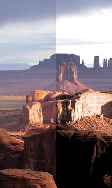 |
|
Dynamic range is a strong function of pixel area, which is proportional to the number of electrons a pixel can store. It is invariably better in DSLRs (which have relatively large pixels; at least 5 microns square) than in compact digital cameras. It can be maximized by setting the camera at the lowest ISO speed.
|
Displaying images with large dynamic ranges (which can be well over 1000:1; 10 f-stops) can be problematic in printed media, which has a maximum dynamic range of about 100:1 (a little over 6 f-stops; 200:1 at the absolute maximum). Reducing contrast can make the image look flat and dull. Some processing is usually required, like applying an "S" curve or dodging and burning (lightening or darkening) portions of the image. Contrast masking is a particularly effective approach. Tonal quality and dynamic range in digital cameras offers additional tips.
Lenses have an intrinsic contrast— the higher the better. But lens contrast isn't exactly intrinsic. It results from flare light— light originating inside and outside the lens's field of view that bounces between lens elements and off the inside of the lens barrel. Flare light tends to fog the image and obscure shadow detail: it reduces dynamic range. To our knowledge there is no solid standard for measuring lens contrast. But you can measure it, or at least compare it for different lenses and apertures, by running Stepchart on a Q-13 (or equivalent) chart mounted on a white board that extends beyond the camera's field of view. (Recall, contrast = gamma.) There would be less flare light, hence higher contrast, with a black board. Actual lens contrast depends strongly on the scene.
Color accuracy
Color accuracy is an important but ambiguous image quality factor. Many viewers prefer enhanced color saturation; the most accurate color isn't necessarily the most pleasing. Nevertheless it is important to measure a camera's color response: its color shifts, saturation, and the effectiveness if its white balance algorithms.
Color accuracy is measured by Colorcheck, using the widely-available 24-patch GretagMacbethTM ColorChecker® and by Multicharts using the 24-patch ColorChecker, ColorChecker SG, IT8.7, QPcard, CMP DC 003, and custom "pie" charts.
Color accuracy is affected by the Bayer color filter array and by the signal processing and white balance algorithms in the camera or RAW converter. Flare light in lenses may reduce color saturation. Multicharts can calculate a color correciton matrix.
|
Original | Color-shifted
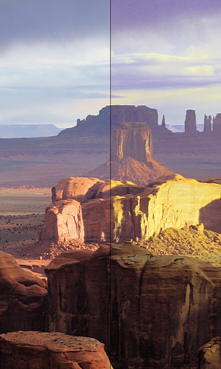 |
Color can be corrected in image editing programs. If a RAW image file has been captured it can be corrected with far more precision with the RAW converter.
Lens distortion
Lens distortion is an aberration that causes straight lines to curve near the edges of images. It can be troublesome for architectural photography and metrology (photographic applications involving measurement). The simplest approximation is the equation, ru = rd + krd3 where ru is the undistorted and rd is the distorted radius. Depending on the sign of k, it can be either "barrel" (shown on the right) or "pincushion."
Lens distortion and coefficients for correcting it are calculated in Distortion, which also includes 5th order and tangent/arctangent distortion models. SFRplus measures distortion in less detail, along with sharpness and several other factors.
Distortion is worst in wide angle, telephoto, and zoom lenses. It often worse for close-up images than for images at a distance. It can be easily corrected in software. Picture Window Pro and PTLens have tools for removing it. |
Original | Barrel-distorted
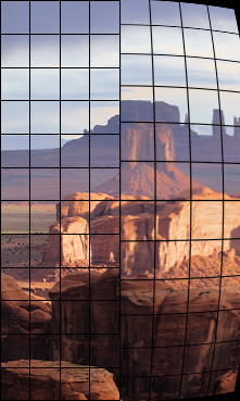 |
Light falloff (vignetting) and sensor nonuniformities
Light falloff (vignetting) darkens images near the corners. It can be significant with wide angle lenses. It is measured by Light Falloff (Uniformity).
Light falloff tends to be worst in wide angle lenses. It often improves when lenses are stopped down. It can be easily corrected in software. Picture Window Pro, PTLens, and several other programs have tools for removing it. Because moderate amounts of light falloff can be pictorially pleasing, it's not always advisable to remove it completely.
Light Falloff (Uniformity) also measures other sensor nonuniformities, including stuck pixels, local sensitivity variations, spots (from dust), and noise. In Imatest Master it has a particularly rich set of displays. |
Original | Vignetted
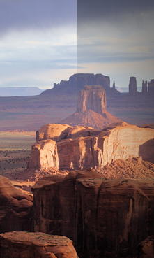 |
Exposure accuracy
Exposure accuracy is not much of a problem with manually-adjustable cameras. You can usually determine it quickly (with the help of the histogram), and if you don't like it, you can change the exposure compensation or the way you meter.
But exposure accuracy can be an issue with fully automatic cameras and with video cameras where there is little or no opportunity for post-exposure tonal adjustment. Some even have exposure memory: exposure may change after very bright or dark objects appear in a scene.
Exposure accuracy can be measured by photographing a gray scale step chart such as the Kodak Q-13 or Q-14 in a scene and analyzing it with Stepchart, or photographing a GretagMacbeth ColorChecker and analyzing it with Colorcheck. |
Original | Overexposed
 |
Lateral chromatic aberration
Lateral chromatic aberration (LCA), also called "color fringing" is a lens aberration that causes colors to focus at different distances from the image center. It is most visible near corners of images. It is explained in Chromatic aberration.
LCA is measured by SFR, using edges at a distance from the image center.
LCA is worst with asymmetrical lenses, including ultrawides, true telephotos and zooms. It is strongly affected by demosaicing. It can be fully corrected in software prior to demosaicing, but only partially corrected afterwards. Picture Window Pro has a fairly effective transformation. In the future, information provided by Imatest (detailed LCA profiles) may improve the degree of correction. |
Original | Color-fringed
 |
Veiling glare (lens flare)
Veiling glare is stray light in lenses and optical systems caused by reflections between lens elements and the inside barrel of the lens. It predicts the severity of lens flare— image fogging (loss of shadow detail and color) as well as "ghost" images— that can occur in the presence of bright light sources in or near the field of view.
Veiling glare is measured by Stepchart using a standard Kodak Q-13 or Q-14 step chart beside a "black hole," i.e., a box lined with black behind a small opening, mounted on a large white board, as described in detail in Veiling glare. |
Original | Veiling glare
 |
Color moiré
Color moiré is artificial color banding that can appear in images with repetitive patterns of high spatial frequencies, like fabrics or picket fences. The example on the right is a detail of a shirt captured by the Canon Rebel XT with its excellent kit lens. The usual image wasn't used because it doesn't contain a repetitive pattern and because color moiré is difficult to simulate.
Color moiré is the result of aliasing (image energy above the Nyquist frequency) in image sensors that employ Bayer color filter arrays, as explained here. It is affected by lens sharpness, the anti-aliasing (lowpass) filter (which softens the image), and demosaicing software. It tends to be worst with the sharpest lenses.
Color moiré is measured by Rescharts Log Frequency, using a sine chart of logarithmically increasing spatial frequency. |
Color Moiré
 |
Software artifacts: noise reduction and sharpening
Software (especially operations performed during RAW conversion) can cause significant visual artifacts, including oversharpening "halos" and loss of fine, low-contrast detail. These artifacts result from nonlinear signal processing (so-called because it varies with the signal). 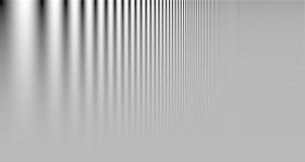 Images may be sharpened (MTF boosted) in the presence of contrasty features like edges and blurred (lowpass filtered) in their absence. This generally improves measured performance (both sharpness and noise/Signal-to-Noise Ratio (SNR)), but it may result in a degradation of perceived image quality, for example, a "plasticy" cartoon-like appearance of skin even though edges are strongly sharpened. This loss of detail cannot be measured with SFR. Images may be sharpened (MTF boosted) in the presence of contrasty features like edges and blurred (lowpass filtered) in their absence. This generally improves measured performance (both sharpness and noise/Signal-to-Noise Ratio (SNR)), but it may result in a degradation of perceived image quality, for example, a "plasticy" cartoon-like appearance of skin even though edges are strongly sharpened. This loss of detail cannot be measured with SFR.
These artifacts can be measured by the Log F-Contrast module in Rescharts, which analyzes the chart shown on the right, which varies logarithmically in spatial frequency on the horizontal axis and in contrast on the vertical axis. |
Original | NR+Sharpening
 |
Data compression and transmission losses
Data compression and transmission losses can have a significant effect on image quality. The right side of the image on the left has been saved as a low quality JPEG. Banding, loss of low-contrast detail, and "waviness" near edges are visible.
A full analysis of data compression and transmission losses is not yet available in Imatest.
Some of these losses, especially the loss of low-contrast detail, can be analyzed with the Log F-contrast module in Rescharts. A more detailed analysis of compression losses is under development. |
Original | Low-quality JPEG
 |
Quality factors for printers
Print Dmax
Dmax = -log10(minimum print reflectivity) is a measure of the deepest black tone a printer/ink/paper combination can reproduce. It is an extremely important print quality factor. Prints with poor Dmax look pale and weak. Dmax = 1.7 is a good value for matte prints; 2.0 is a good value for glossy, semigloss, and luster prints. There have been reports that the new Epson Ultrachrome K3 printers have Dmax as high as 2.3 with Premium Luster paper. That would be outstanding.
Dmax is measured by Print Test, along with the Printer's tonal response curve and the color factors described below. Print test requires a decent flatbed scanner, and for best accuracy, a Step chart.
Dmax is affected by the printer, paper, and ink. The response curve is also affected by the ICC profile. Print Test can help with the selection of supplies and diagnosis of printing problems. |
Original | Reduced Dmax
 |
Print color gamut
Print color gamut is the range of colors a printer/ink/paper combination can reproduce. It is an important quality factor, though its importance may be somewhat overrated. (This statement is bound to generate controversy.) Relatively unsaturated colors such as skin tones dominate our impression of print quality. Such colors must be reproduced accurately. Gamut affects only highly saturated colors. Overall color response, especially for low to moderately saturated colors, is more important than gamut.
Print color gamut and overall color response are measured by Print Test, along with the density factors described above.
Print gamut is affected by the printer, paper, ink, and working color space. Color response is also affected by the ICC profile and rendering intent. Print Test can help with the selection of profiles, software settings, and the diagnosis of color problems. |
Original | Reduced gamut
 |
Links
Bror Hultgren (ImagIntegration.com), an imaging scientist with 27 years experience at Polaroid, has developed algorithms and software that relates image quality factors (especially MTF, noise spectrum, white balance, and memory colors) to perceived image quality. Bror is available for consulting.
Direct Digital Image Capture of Cultural Heritage from RIT is a gold mine of information. Links to a number of reports on image quality targeted at museums and cultural institutions. The 78-page Final Project Report by Berns, Frey, Rosen, Smoyer and Taplin, July 2005, is probably the best summary unless you have time for Erin P (Murphy) Smoyer's 345 page Master's thesis (about twice the length of the average Ph.D. thesis).
The Research Library Group (RLG) has published an excellent series of articles, Guides to Quality in Visual Resource Imaging (2000). These articles are the predecessors to the above-mentioned RIT Direct Digital Image Capture work.
The European Broadcasting Union (EBU) has a library of technical papers (the EBU Tech 3000 series), some related to TV image quality, for example, T3249, Measurement and Analysis of the Performance of Film and Television Camera Lenses (1995), and T3281, Methods for the Measurement of Characteristics of CCD Cameras (1995).
Volker Gilbert has written an excellent French language description of Imatest. (PDF version)
SMIA (Standard Mobile Imaging Architecture), a consortium founded by Nokia and STMicroelectronics, has published a Camera Characterization Specification for image quality measurements in camera phones. To obtain the spec you must join SMIA. It's free; all you need to do is answer a brief questionnaire.
Paul van Walree has an excellent page on Optics, covering several sources of degradation.
The University of Texas Laboratory for Image & Video Engineering is doing some interesting work on image and video quality assessment, which approaches the problem using information theory, natural scene statistics, wavelets, etc. Challenging material!
Details of many Imatest algorithms are included in Appendix C, Video Acquisition Measurement Methods (pp. 91-125), of the Public Safety SoR (Statement of Requirements) volume II v 1.0, released by SAFECOM, prepared by ITS (a division of NTIA, U.S. Department of Commerce). No credit is given, but the style and illustrations will be recognizable.
Sharpness
What is it and how is it measured?
Image sharpness
Sharpness is arguably the most important photographic image quality factor: it's the factor most closely related to the amount of detail an image can render. But it's not the only important factor. Others measured by Imatest include chromatic aberration (closely related to sharpness), noise, dynamic range (closely related to noise), and color accuracy.
Sharpness is defined by the boundaries between
zones
of different tones or colors. It is illustrated by the bar pattern of
increasing
spatial frequency, below. The top portion represents a target used to
test
a camera/lens combination. It is sharp;
its boundaries are abrupt, not gradual. The bottom portion illustrates
the effect of a high quality 35mm lens on a 0.5 millimeter long image
of
the pattern (on the film or digital sensor plane). It is blurred.
All lenses, even the finest, blur images to some degree. Poor lenses
blur images more than fine ones.

One way to measure sharpness is to use the rise
distance of the edge, for example, the distance (in pixels, millimeters, or fraction of image height) for the pixel level to go from 10% to 90% of its final
value. This is called the 10-90% rise distance. Although rise distance
is a good indicator of image sharpness, it has one limitation. It is
poorly suited for calculating the sharpness of a complete imaging
system
from the sharpness of its components, for example, from a lens, digital
sensor, and software sharpening algorithm.
To get around this problem, measurements are made in frequency
domain, where frequency is measured in cycles
or line pairs per distance
(typically millimeters in film measurements, but may also be inches, pixels, or image height). Line
pairs per millimeter (lp/mm)
is the most common spatial frequency unit for film, but cycles/pixel is convenient for digital sensors. The
image below is a sine wave— a pattern of pure tones— that varies from
low to high spatial frequencies, in this case from 2 to 200 lp/mm, over
a distance of 0.5 millimeters. The top portion is the
original
sine pattern. The bottom portion illustrates the effects of the same
high
quality 35mm lens, which reduces pattern contrast at high
spatial frequencies.
The relative contrast at a given spatial frequency (output
contrast/input contrast) is called the Modulation Transfer
Function (MTF) or Spatial Frequency Response (SFR).
Illustration of Modulation
Transfer Function (MTF)
(Spatial frequency response (SFR) )
|
The upper plot displays the sine and bar patterns: original
and after blurring by the lens.
The middle plot displays the luminance of the bar pattern after
blurring
by the lens (the red curve).
Contrast
decreases at high spatial frequencies.
The lower plot displays the corresponding MTF (SFR) curve (the
blue curve).
By definition, the low frequency MTF limit is always 1 (100%). For this lens,
MTF is 50% at 61 lp/mm and 10% at 183 lp/mm.
|
 |
Both frequency and MTF are displayed on logarithmic scales with exponential notation (100 = 1; 101 = 10; 102 = 100, etc.). Amplitude is displayed on a linear scale.
The beauty of using MTF (Spatial Frequency Response) is that the MTF of a complete imaging system is the product of the the MTF of its individual components.
Green is
for geeks. Do you
get excited by a good equation? Were you passionate about your college
math classes? Then you're probably a math geek— a member of a misunderstood but highly elite fellowship. The text in green is for
you. If you're normal or mathematically challenged, you may skip these
sections. You'll never know what you missed.
MTF is related to edge response by a mathematical
operation known as the
Fourier transform.
MTF is the Fourier
transform of the impulse response— the response to a narrow line,
which
is the derivative (d/dx) of the edge response. Fortunately, you don't
need
to understand Fourier transforms or calculus to understand MTF.
Traditional "resolution" measurements involve observing an image of
a bar pattern (usually the USAF 1951 chart) on film, and looking for
the
highest spatial frequency (in lp/mm) where a pattern is visible. This
corresponds
to an MTF of about 2-5%. Because this is the spatial frequency where
image
information disappears— where it isn't
visible, it is not a good indicator of image sharpness.
Experience has shown that the
best indicators of image sharpness are the spatial frequencies where MTF is
50% of its low frequency value
(MTF50) or 50% of its peak value (MTF50P).
MTF50 or MTF50P are ideal parameters for comparing the sharpness of different
cameras
for several reasons: (1) Image contrast is half its low frequency
or peak values,
hence detail is still quite visible. (2) The eye is relatively
insensitive
to detail at spatial frequencies where MTF is low: 10% or less. (3) The
response of virtually all cameras falls off rapidly in the vicinity of
MTF50 and MTF50P. MTF50P may better for oversharpened cameras that have peaks in their MTF response.
Although
MTF can be estimated directly from images of sine patterns (see Rescharts Log Frequency, Log F-Contrast, and Star Chart),
a sophisticated technique, based on the ISO
12233 standard, "Photography - Electronic still picture
cameras
- Resolution measurements," provides more accurate and repeatable
results.
A slanted-edge image, described below, is photographed, then analyzed
by Imatest SFR or Rescharts Slanted-edge SFR. (SFR
stands for Spatial Frequency Response.)
Origins of Imatest SFR The algorithms for calculating MTF/SFR were adapted from a Matlab program, sfrmat, written by Peter Burns ( ) to implement the ISO 12233 standard. Imatest SFR incorporates numerous improvements, including improved edge detection, better handling of lens distortion, a nicer interface, and far more detailed output. The original Matlab code is available on the I3A ISO tools download page by clicking on ISO 12233 Slant Edge Analysis Tool sfrmat 2.0. In comparing sfrmat 2.0 results with Imatest, note that if no OECF (tonal response curve) file is entered into sfrmat, it assumes that there is no tonal response curve, i.e., gamma = 1. In Imatest, gamma is set to a default value of 0.5, which is typical of digital cameras. To obtain good agreement with sfrmat, you must set gamma to 1. ) to implement the ISO 12233 standard. Imatest SFR incorporates numerous improvements, including improved edge detection, better handling of lens distortion, a nicer interface, and far more detailed output. The original Matlab code is available on the I3A ISO tools download page by clicking on ISO 12233 Slant Edge Analysis Tool sfrmat 2.0. In comparing sfrmat 2.0 results with Imatest, note that if no OECF (tonal response curve) file is entered into sfrmat, it assumes that there is no tonal response curve, i.e., gamma = 1. In Imatest, gamma is set to a default value of 0.5, which is typical of digital cameras. To obtain good agreement with sfrmat, you must set gamma to 1. |
The slanted-edge test for Spatial Frequency Response
Slanted-edge test charts can be created with Imatest Test Charts (SVG charts are especially recommended) or downloaded from How to test lenses with Imatest. The bitmap chart has horizontal and vertical edges for best print quality. It should be tilted (about 2-8 degrees) before it is photographed.
A printable vector-graphics version of the ISO chart is available courtesy of Stephen H. Westin of the Cornell University Computer Graphics Department. It should be printed as large as possible (24 inches high if possible) so edge sharpness is not limited by the printer itself. (There may be some jaggedness in the slanted edges; not a problem with the recommended printable target.)
A typical portion is shown on the right: a crop of a vertical edge (slanted about 5.6 degrees), used to calculate horizontal MTF response. An advantage of the slanted edge test is that the camera-to-target distance isn't critical. It doesn't enter into the equation that converts the image into MTF response. Imatest Master can calculate MTF for edges of virtually any angle, though exact vertical, horizontal, and 45° can have numerical problems.
|
|
Slanted edge algorithm (calculation details)
The MTF calculation is derived from
ISO standard 12233. Some details are contained in Peter Burns' SFRMAT 2.0 User's Guide, which can be downloaded from the
I3A ISO tools download page by clicking on
Slant Edge Analysis Tool sfrmat 2.0. The Imatest calculation contains a number of refinements and enhancements, including more accurate edge detection and compensation for lens distortion (which could affect MTF measurements). The original ISO calculation is performed when the
ISO standard SFR checkbox in the
SFR input dialog box is checked. It is normally left unchecked.
- The cropped image is linearized, i.e., the pixel levels are adjusted to remove the gamma encoding applied by the camera. (Gamma is adjustable with a default of 0.5).
- The edge locations for the Red, Green, Blue, and luminance channels (Y = 0.3*Red + 0.59*Green + 0.11*Blue) are determined for each scan line (horizontal lines in the above image).
- A second order fit to the edge is calculated for each channel using polynomial regression. The second order fit removes the effects of lens distortion. In the above image, the equation would have the form, x = a0 + a1 y + a2 y2.
- Depending on the value of the fractional part fp = xi - int(xi ) of the second order fit at each scan line, the shifted edge is added to one of four bins (bin 1 if 0 ≤ fp < 0.25; bin 2 if 0.25 ≤ fp < 0.5; bin 3 if 0.5 ≤ fp < 0.75; bin 4 if 0.75 ≤ fp < 1. (Correction 11/22/05: the bin does not depend on the detected edge location.)
- The four bins are combined to calculate an averaged 4x oversampled edge. This allows analysis of spatial frequencies beyond the normal Nyquist frequency.
- The derivative (d/dx) of the averaged 4x oversampled edge is calculated. A windowing function is applied to force the derivative to zero at its limits.
- MTF is the absolute value of the Fourier transform (FFT) of the windowed derivative.
Additional details of the calculation can be found in Appendix C, Video Acquisition Measurement Methods (especially pp. 102-103), of the Public Safety SoR (Statement of Requirements) volume II v 1.0 (6 MB download), released by SAFECOM, prepared by ITS (a division of NTIA, U.S. Department of Commerce).
Imatest SFR results
35mm camera lens tests use line
pairs per millimeter (lp/mm) as the
units of spatial frequency. This works fine for comparing lenses
because
all 35mm cameras have the same 24x36 mm picture size. But digital sensor digital
varies widely, from under 6 mm diagonal in
ultra-compact
models to 43 mm diagonal for full-frame DSLRs— even larger for medium format
backs.
The number of pixels also varies. For this reason, spatial
frequency should be measured in units that indicate the response over the total
sensor height rather than the response per distance.
For this purpose we use line widths per picture height
(LW/PH). LW/PH is equal to 2 * lp/mm * (picture height in mm). Where total
picture height is involved, line widths is
customarily used instead of pairs (where one line pair
equals two line widths).
The use of picture height gives a slight advantage
to compact digital cameras, which have an aspect ratio (width:height)
of
4:3, compared to 3:2 for digital SLRs. Compact digital cameras have
slightly
more vertical pixels for a given number of total pixels. For example, a
5.33 megapixel compact digital camera would have 2000 vertical pixels—
as many as a 6 megapixel DSLR.
Another measure of spatial frequency used
with digital cameras is cycles
or line pairs
per pixel
(c/p
or lp/p).
This gives an indication of how well individual pixels perform.
There is no need to use actual distances (millimeters or inches) to
evaluate
digital camera image quality, although such measurements are available in Imatest SFR.
Imatest SFR program output contains results on the left and input data on the right (a
thumbnail of the entire image, the region of interest (ROI), and
selected EXIF data).
 Results from the ISO 1233 image for the Canon EOS-10D.
(top) A narrow image that illustrates the tones of the
averaged
edge. It is aligned with the edge profile (spatial domain) plot,
immediately
below.
(middle) Spatial
domain plot: The average edge profile (linearized, i.e., proportional to light energy). The key result is the 10-90%
edge rise distance, shown in pixels and in the
number of rise distances per picture height. The
red values are for standardized
sharpening. Other parameters include overshoot and undershoot (if applicable). This plot can optionally display the line spread function (LSF: the derivative of the edge), or the edge in pixels (gamma-encoded).
(bottom) Frequency domain plot: The Spatial Frequency Response (MTF), shown to twice the Nyquist frequency. The key result is MTF50, the 50% MTF frequency, which corresponds to perceived image sharpness. It is given in cycles per pixel (c/p) and line widths per picture height (LW/PH). Other results include MTF at NYQ, the MTF at the Nyquist frequency (0.5 cycles/pixel; sampling rate/2), which indicates the probable severity of aliasing. The Nyquist frequency is displayed as a vertical blue line.
For this camera, which is moderately sharpened, MTF50P (only shown when Standardized sharpening display is unchecked) is identical to MTF50.
SFR Results: MTF (sharpness) plot describes this Figure in detail.
Interpreting MTF50
This section was written before the addition of SQF (Subjective Quality Factor) to Imatest (Ver. 2.1, November 2006).
SQF allows a more refined estimate of perceived print sharpness. |
What MTF50 do you need? It depends on print size. If you plan to print gigantic posters (20x30 inches or over), the more the merrier. Any high quality 4+ megapixel digital camera (one that produces good test results; MTF50(corr) > 0.3 cycles/pixel) is capable of producing excellent 8.5x11 inch (letter-size; A4) prints. At that size a fine DSLR wouldn't offer a large advantage in MTF. With fine lenses and careful technique (a different RAW converter from Canon's and a little extra sharpening), my 6.3 megapixel Canon EOS-10D (corrected MTF50 = 1340 LW/PH) makes very good 12x18 inch prints (excellent if you don't view them too closely). Prints are sharp from normal viewing distances, but pixels are visible under a magnifier or loupe; the prints are not as sharp as the Epson 2200 printer is capable of producing. Softness or pixellation would be visible on 16x24 inch enlargements. The EOS-20D has a slight edge at 12x18 inches; it's about as sharp as I could ask for. There's little reason go go to a 12+ megapixel camera lie the EOS 5D, unless you plan to print larger. Sharpness comparisons contains tables, derived from images downloaded from two well-known websites, that compare a number of digital cameras. Several outperform the 10D.
The table below is an approximate guide to quality requirements. The equation for the left column is
| MTF50(Line Widths / inch on the print) = |
MTF50(LW/PH)
Print height in inches
|
MTF50 in
Line Widths/inch
on the print |
Quality level— after post-processing, which may include some additional sharpening |
| 150 |
Excellent— Extremely sharp at any viewing distance. About as sharp as most inkjet printers can print. |
| 110 |
Very good— Large prints (A3 or 13x19 inch) look excellent, though they won't look perfect under a magnifier. Small prints still look very good. |
| 80 |
Good— Large prints look OK when viewed from normal distances, but somewhat soft when examined closely. Small prints look soft— adequate, perhaps, for the "average" consumer, but definitely not "crisp." |
Example of using the table: My Canon EOS-10D has MTF50 = 1335 LW/PH (corrected; with standardized sharpening). When I make a 12.3 inch high print on 13x19 inch paper, MTF50 is 1335/12.3 = 108 LW/in: "very good" quality; fine for a print that size. Prints look excellent at normal viewing distances for a print this size.
This approach is more accurate than tables based on pixel count (PPI) alone (though less refined than SQF, below). Pixel count is scaled differently; the numbers are around double the MTF50 numbers. The EOS-10D has 2048/12.3 = 167 pixels per inch (PPI) at this magnification. This table should not be taken as gospel: it was first published in October 2004, bandit may be adjusted in the future.
Subjective Quality Factor (SQF)
MTF is a measure of device or system sharpness, only indirectly related to the sharpness perceived when viewing a print. A more refined estimate of perceived print sharpness must include assumptions about viewing distance (typically proportional to the square root of print height) and the human visual system (the human eye's Contrast Sensitivity Function (CSF)). Such an formula, called Subjective Quality Factor (SQF) was developed by Eastman Kodak scientists in 1972. It has been verified and used inside Kodak and Polaroid, but it has remained obscure until now because it was difficult to calculate. Its only significant public exposure has been in Popular Photography lens tests. SQF was added to Imatest in October 2006.
A portion of the Imatest SFR SQF figure for the EOS-10D is shown on the right. SQF is plotted as a function of print size. Viewing distance (pale blue dashes, with scale on the right) is assumed to be proportional to the square root of picture height. SQF is shown with and without standardized sharpening. (They are very close, which is somewhat unusual.) SQF is extremely sensitive to sharpening, as you would expect since sharpening is applied to improve perceptual sharpness.
The table below compares SQF for the EOS-10D with the MTF50 from the table above.
MTF50 in
Line Widths/inch
on the print |
Corresponding print height for the EOS-10D (MTF50 = 1335 LW/PH) |
SQF at this print height |
Quality level— after post-processing, which may include some additional sharpening. Overall impression from viewing images at normal distances as well as close up. |
| 150 |
8.9 inches = 22.6 cm |
93 |
Excellent— Extremely sharp. |
| 110 |
12.1 inches = 30.8 cm |
90 |
Very good. |
| 80 |
16.7 inches = 42.4 cm |
86 |
Good— Very good at normal viewing distance for a print of this size, but visibly soft on close examination. |
An interpretation of SQF is give here. Generally, 90-100 is considered excellent, 80-90 is very good, 70-80 is good, and 60-70 is fair. These numbers (which may be changed as more data becomes available) are the result of "normal" observers viewing prints at normal distances (e.g.., 30-34 cm (12-13 inches) for 10 cm (4 inch) high prints). The judgments in the table above are a bit more stringent— the result of critical examination by a serious photographer. They correspond more closely to the "normal" interpretation of SQF when the viewing distance is proportional to the cube root of print height (SQF = 90, 86, and 80, respectively), i.e., prints are examined more closely than the standard square root assumption.
An SQF peak over about 105 may indicate oversharpening (strong halos near edges), which can degrade image quality. SQF measurements are more valid when oversharpening is removed, which is accomplished with standardized sharpening.
Some observations on sharpness
- Frequency and spatial domain plots convey similar information,
but in a
different form. A narrow edge in spatial domain corresponds to a broad
spectrum in frequency domain (extended frequency response), and
vice-versa.
- Sensor response above the Nyquist frequency is garbage— aliasing,
visible as
Moire patterns of low spatial frequency. In Bayer sensors (all
sensors
except Foveon) Moire patterns appear as color fringes. Moire in Foveon sensors is far less bothersome because it's monochrome and because the effective Nyquist frequency of the Red and Blue channels is lower than for Bayer sensors.
- Since MTF is the product of the sensor response, demosaicing algorithm, and sharpening, and since sharpening with a radius less than 2 boosts MTF at the Nyquist frequency, the MTF at and above the Nyquist frequency is not an unambiguous indicator of aliasing problems. It may, however, be interpreted as an indicator of potential problems.
- Results are calculated for the R, G, B, and Luminance (Y) channels, where Y = 0.3*R
+ 0.59*G + 0.11*B. The Y channel is normally displayed in the foreground, but any of the other channels can selected. All are included in the .CVS output file.
- Horizontal and vertical resolution can be different for CCD
sensors, and
must be measured separately. They're nearly identical for CMOS sensors.
Recall, horizontal resolution is measured with a vertical edge and
vertical
resolution is measured with a horizontal edge.
- Resolution is not the only important criterion for evaluating
image
quality.
Noise is nearly as important. The Shannon
information capacity is an experimental metric that combines the two.
The
ideal response would have high MTF below
the Nyquist frequency and low MTF at and above it.
Links
Bob Atkins has an excellent introduction to MTF and SQF. SQF (subjective quality factor) is a measure of perceived print sharpness that incorporates the contrast sensitivity function (CSF) of the human eye. It will be added to Imatest Master in late October 2006.
This
page has some interesting material on Fuji sensors and the history
of the slanted-edge test.
Spatial
Frequency
Response of Color Image Sensors: Bayer Color Filters and Foveon X3
by Paul M. Hubel, John Liu and Rudolph J. Guttosch, Foveon, Inc., Santa
Clara, California. Uses slanted edge testing.
Optikos makes instruments for measuring lens MTF. Their 64 page PDF document, How to Measure MTF and other Properties of Lenses, is of particular interest.
Zeiss makes instruments for measuring MTF. You can't deep link to their site; you must go to the North America page, click on Camera/Cine Lenses in the dropdown menu, then search for MTF. The MTF-Tester K8 is used for many manufacturer's lens tests.
SQF
Subjective Quality Factor
Introduction to SQF
SQF (Subjective Quality Factor) is a measurement of perceived print sharpness that has been used for years in the photographic industry but has remained unfamiliar to most photographers. It includes the effects of
- MTF: the imaging system's Modulation Transfer Function, which is synonymous with Spatial Frequency Response (SFR),
- CSF: the human eye's Contrast Sensitivity Function,
- print height, and
- viewing distance.
SQF was introduced in the paper, "An optical merit function (SQF), which correlates with subjective image judgments ," by E. M. (Ed) Granger and K. N. Cupery of Eastman Kodak, published in Photographic Science and Engineering, Vol. 16, no. 3, May-June 1973, pp. 221-230. (If you do an Internet search, note that Granger's name is often misspelled Grainger.) It has been used by Kodak and Polaroid for product development and by Popular Photography for lens tests. This technical paper verified its correlation with viewer preference. But SQF is rarely mentioned on photography websites with the notable exception of Bob Atkins' excellent description, which includes an explanation of Pop Photo's methods.
SQF has remained obscure for only one reason. It was difficult to measure— until now.
SQF and MTF
The following table compares MTF and SQF. In essence, MTF is a measurement of device or system sharpness; SQF is a measurement of perceived print sharpness. SQF is derived from MTF, the contrast sensitivity function (CSF) of the human visual system, and an assumption about the relationship between print height and viewing distance.
| MTF (Modulation Transfer Function) |
SQF (Subjective Quality Factor) |
| Measures image contrast as a function of spatial frequency. Describes device or system sharpness. Indirectly related to perceived image sharpness in a print or display. |
Measures perceived sharpness as a function of print or display height and viewing distance. Describes viewer experience. Requires an assumption about viewing distance (can be constant or proportional to the square root or cube root of print height). |
| Omits viewing distance and the human visual system. |
Includes the effects of viewing distance and the human visual system. |
| Abstract: Plots of MTF (contrast) vs. spatial frequency require technical skill to interpret. |
Concrete: Plots of SQF (perceived sharpness) vs. print height require little interpretation. SQF has the same subjective meaning regardless of print size. It can be used to precisely answer questions like, "How much larger can I print with a 12.8 Megapixel full-frame DSLR than with an 8.3 Megapixel APS-C DSLR?" |
| 1.0 at low spatial frequencies. Decreases at high spatial frequencies, but may peak at intermediate frequencies due to sharpening. A peak over 1.4 indicates oversharpening, which can result un unpleasant "halos" at edges, especially for large print sizes. |
100 (%) for small print heights. Decreases for large print heights, but may increase at intermediate print heights due to sharpening. A peak value over about 105% may indicate oversharpening (and over 108% definitely indicates oversharpening). In such cases you should examine the MTF plot and edge profile. |
| The frequency where it drops by half (MTF50) is a reasonable indicator of relative perceived sharpness, but requires interpretation and is not as precise as SQF. |
An SQF difference of 5 corresponds to a clearly perceptible difference in sharpness, and can be used as the basis of a ranking system. |
| Familiar to imaging scientists Gradually becomming familiar to a wider public, though vanishing resolution is still better known. |
Unfamiliar Used internally in Kodak and Polaroid, but difficult to measure prior to the advent of digital imaging. |
| Both are strongly affected by sharpening, which is routinely performed to improve perceived sharpness, hence SQF would be expected to increase. SQF measurements with standardized sharpening can help determine the optimum sharpening radius for a desired print size. |
Starting with Imatest 2.0.3, released in October 2006, SQF is calculated as a part of the SFR module. All you need to do is check the SQF checkbox in the SFR input dialog box. The SQF calculation is completely backwards-compatible: you can calculate SQF for all existing image files that contain slanted-edges for SFR analysis. Here is a sample result.
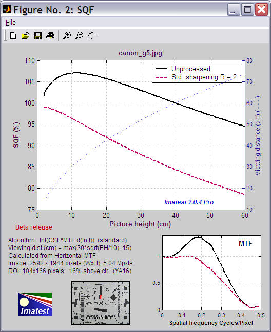
The large plot on top shows SQF without ( —— ) and with ( - - - ) standardized sharpening for print heights from 5 to 60 cm (~2 to 24 inches), assuming viewing distance (cm) = 30 √(picture height/10). For this mildly oversharpened camera, standardized sharpening decreases the sharpness (removes the strong overshoot), and hence reduces the SQF, which is highly sensitive to sharpening. The large plot also shows viewing distance ( - - - ). The plot on the lower right is the MTF without and with standardized sharpening, displayed in the main SFR/MTF figure, but repeated here to make this figure self-contained. The lower middle contains a thumbnail of the image showing the selected ROI in red. The text on the left contains calculation details and image properties.
What do the SQF numbers mean?
Ed Granger developed SQF to be linearly proportional to perceived sharpness. A change in SQF of 5 corresponds to a perceptible change in in sharpness— somewhat more than one "Just Noticeable Difference" (JND). Since SQF is a new feature of Imatest (version 2.0.3, Oct. 2006), we haven't had time to build our own database of SQF impressions. So we'll draw on the experience of others.
Popular Photography has been using SQF for testing lenses for years. They've developed the only generally-available SQF ranking system. Their scale isn't quite linear. {C, C+} takes up 20 SQF units; twice as many as {A, A+}, {B, B+}, or D. But it seems to be a good starting point for interpreting the numbers.
| A+ |
A |
B+ |
B |
C+ |
C |
D |
F |
| 94-100 |
89-94 |
84-89 |
79-84 |
69-79 |
59-69 |
49-59 |
Under 49 |
We encourage readers to examine Popular Photography's lens test results and to search its site for SQF. Imatest results should correlate with Pop Photo's results, but there are a few significant differences.
- Pop Photo measures SQF for lenses alone, while Imatest measures SQF for the entire imaging system. This means that Imatest results are sensitive to signal processing (sharpening and noise reduction; often applied nonlinearly) in the camera and RAW converter. This makes is difficult to compare lenses from measurements taken on different cameras. On the other hand, it means that you know what your camera/lens combination can achieve, and it's excellent for comparing lenses measured on one camera type (with consistent settings).
- Pop Photo's algorithm for calculating SQF (the SQF equation and the viewing distance assumption; both discussed below) is not known.
| The scale on the right was developed by Bror Hultgren of Image Integration, based on extensive category scaling tests. According to Bror, the perceived quality level depends on the set of test images (particularly how bad the worst of them is) as well as the task (e.g., a group of cameraphone users would rank images differently from a group of art gallery curators), but the relationships between categories remains relatively stable. These levels are comparable to Popular Photography's scale. |
 |
Additional considerations in interpreting SQF:
- SQF has the same interpretation regardless of print size. That means a print with SQF = 92 would have the same quality "feel" for a 4x6 print as for a 24x36 inch print. This is in contrast to MTF measurements, where MTF measured at the print surface is interpreted differently for different sizes of prints: you tend to accept lower MTF for larger prints because you view them from larger distances (though the relationship, described here, is far from linear). Viewing distance is built into SQF.
- The SQF calculation omits printer sharpness (for now). It assumes that modern high quality inkjet printers can print as sharp as the unassisted eye can see at normal viewing distances— a fairly safe assumption for large prints (≥ 20 cm high).
Measuring SQF
SQF is measured as a part of Imatest SFR. All you need to do is check the SQF checkbox in the Imatest SFR input dialog box. Settings will be remembered in succeeding runs.
Clicking on Options to the right of the SQF checkbox opens this dialog box for setting SQF options. Most of the time you'll want to leave them (except for Maximum print height, which doesn't affect the calculations) at their default values, which you can always restore by pressing Reset .
CSF equation selects the equation for the Contrast Sensitivity function. There are two choices.
- Flat from 3 to 12 cpd (where cpd is cycles per degree) is the simplifying approximation originally used by Granger and Cupery in 1972, and by a number of authors since. (Granger actually used 10 to 40 cycles/mm at the retina, which translates to 3-12 cycles/degree when the eye's focal length of 17 mm is tossed into the equation.) This setting is recommended only for comparing results between the new and old explanation.
- Equation: (a + bf) exp(-bf) (the default setting) is discussed in detail in the section on Contrast Sensitivity function. This setting is recommended.
SQF integral is the form of the integral used in the SQF calculation. The default setting, 2. Integral( CSF(f) MTF(f) d(ln f) ), is recommended. The other values are experimental and not recommended; they are discussed below.
Viewing distance allows four choices.
- Fixed assumes a fixed viewing distance, which can be selected in the Base viewing distance... box.
- Square root of PH (15 cm min.) (the default setting) assumes that viewing distance is proportional to the square root of the picture height, (d = (base distance) (PH /10)1/2 ), with a minimum of 15 cm. This is the recommended setting, appropriate for typical gallery viewing. We tend to look at large prints at greater distances than small prints. With this assumption, if you viewed a 4x6 inch print at 12 inches (a number often found in the literature), you would view a 16x24 inch print at 24 inches.
- Cube root of PH (15 cm min.) assumes that viewing distance is proportional to the cube root of the picture height, (d = (base distance) (PH /10)1/3 ). With this assumption, if you viewed a 4x6 inch print at 12 inches (a number often found in the literature), you would view a 32x48 inch print at 24 inches. This seems to be a little close, but it could be appropriate in some situations.
- Fixed print height; Distance from 1 cm to max. This option is different from the others. Maximum viewing distance (cm) and Print height (cm) are entered instead of Base viewing distance and Maximum print height. SQF is plotted for viewing distances from 1 cm to the maximum for the fixed print height.
Of course Viewing distance is a broad average: we often move in and out when we critically examine a print. But some assumption must be made for the SQF calculation to proceed. We believe that choice 2, Viewing distance proportional the square root of the picture height, best represents the typical impression of sharpness for a range of prints. If we come across research that suggests a different fuction, we'll add it to the choices.
Base distance Defined according to the Viewing distance setting. It should be left at its default value of 30 cm (12 inches) unless there is good reason to change it. 34 centimeters has also been used for measuring perceived quality in 10 cm high (4x6 inch) prints.
For Viewing distance = 1. Fixed, base distance is the viewing distance in cm.
For Viewing distance = 2. Square root or 3. Cube root (of picture height), base distance is the viewing distance for 10 cm (4 inch) high prints.
Maximum print height is the maximum to plot. (Note that the height setting assumes landscape orientation: wider than tall.) It has no effect on the calculations. The default is 40 cm (16 inches), which is about as large as prints from consumer digital cameras get. Picture heights of 60 cm (24 inches) and larger are of interest to users of professional-quality digital SLRs. 20 cm is a stretch for cameraphone images.
Reset resets settings to their default values. (It doesn't affect Maximum print height, which has no effect on the calculations.) We recommend keeping all settings at their default values, unless there is good reason to change them. This will help ensure standardized measurements and minimize confusion.
The SQF equation
Following the convention elsewhere in the Imatest site, we put the math in green boxes, which can be skipped by non-technical readers. The gist of the box below is that Granger presented the full equation for calculating SQF in 1972, but he used a simplified approximation for his calculations. Although the exact equation is strongly recommended, Imatest can use the simplified approximation where needed for comparing new and old calculations. In reviewing older publications, you should determine which calculation was used.
The SQF equation
The exact equation for SQF implied by Granger is,
SQF = K ∫CSF( f ) MTF( f ) d(log f )
= K ∫(CSF( f ) MTF( f ) / f ) d f for all angular frequencies f
where
CSF( f ) is the contrast sensitivity function of the human eye, discussed below; CSF( f ) is close to zero for f > 60 cycles/degree),
MTF( f ) is the Modulation Transfer function (equivalent to Spatial Frequency Response) of the optical system: the primary output of Imatest SFR,
log (often written ln) is the natural logarithm, i.e., loge. d(log f ) = d f / f .
K = 100% / ∫ CSF( f ) d(log f ) = 100% / ∫(CSF( f ) / f ) d f is the normalization constant: SQF would equal 100% for MTF( f ) with a constant value of 1.
The Nyquist frequency is the upper frequency limit for the integral; energy above Nyquist does not contribute to image quality.
Since Granger had limited access to sophisticated computers (the average personal computer today has about as much power as the entire Pentagon had in 1972), he used an an approximation for his calculations assuming that CSF( f ) is roughly constant from 3 to 12 cycles/degree.
SQF = K ∫ MTF( f ) d(log f ) = K ∫(MTF( f ) / f ) d f for 3 cpd < f < 12 cpd; 0 otherwise;
K = 100% / ∫ d(log f ) = 100% / ∫ d f /f for 3 cpd < f < 12 cpd is the normalization constant.
K = 100% / (log(12)-log(3)) = 72.1348%
Although Imatest offers the option of using this approximation (as a check on older calculations), the exact equation is recommended. The integration limits used by Granger and Cupery were 10 and 40 cycles/mm in the retina of the eye, which translate to 3 and 6 cycles/degree when the eye's focal length (FL = 17 mm) is considered. f (cycles/degree) = f (cycles/mm) (π FL) / 180.
To calculate SQF it is necessary to relate spatial frequency in cycles/degree, which is used for the eye's response CSF( f ), to spatial frequency in cycles/pixel, which is calculated by Imatest SFR.
f (cycles/degree) = f (cycles/pixel) (π nPH d ) / (180 PH )
where
nPH is the number of vertical pixels (along the Picture Height, assuming landscape orientation),
d is the viewing distance
PH is the picture height in units of distance (centimeters is used in Imatest displays). Note that nPH / PH is the actual value of pixels per distance. The "pixels per inch" value of image files rarely corresponds to real prints.
Noisy images
In images with long transitions (10-90% risetime r1090 over 2 pixels) and high noise, increasing the noise can increase the SQF, unless we take preventative steps. What we do is to recognize that most signal energy is at spatial frequencies below 1/r1090. At frequencies over 1/r1090 we do not allow MTF to increase: MTF( fn ) = min( MTF( fn-1 ), MTF( fn ) ). This has little or no effect on the MTF due to the edge, but prevents noise spikes from unduly increasing SQF. |
|
Contrast sensitivity function CSF
The human eye's contrast sensitivity function (CSF) is limited by the eye's optical system and cone density at high spatial (or angular) frequencies and by signal processing in the retina (neuronal interactions; lateral inhibition) at low spatial frequencies. Various studies place the peak response at bright light levels (typical of print viewing conditions) between 6 and 8 cycles per degree. We have chosen a formula, described below, that peaks just below 8 cycles/degree.
You may learn something about your own eye's CSF by viewing the chart below at various distances and observing where the pattern appears to vanish. Chart contrast is proportional to (y/h)2, for image height h. To my eyes (which underwent Lasik refractive surgery in 1998 to correct for 10 diopter nearsightedness) it appears that the peak in the curve on the right should be considerably broader. But this isn't quite the case because of the eye's nonlinear response to contrast. Although the chart below appears to decrease in contrast linearly from top to bottom, the middle of the chart has 1/4 the contrast as the top. |
 |
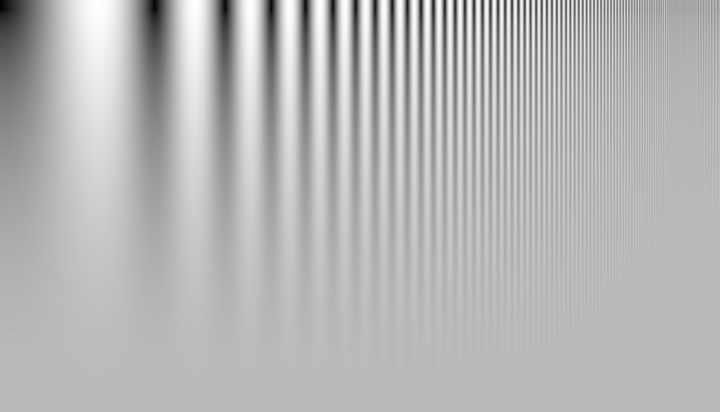
Log frequency-Contrast chart, created by Test Charts.
We have chosen a formula that is relatively simple, recent, and provides a good fit to data. The source is J. L. Mannos, D. J. Sakrison, ``The Effects of a Visual Fidelity Criterion on the Encoding of Images'', IEEE Transactions on Information Theory, pp. 525-535, Vol. 20, No 4, (1974), cited on this page of Kresimir Matkovic's 1998 PhD thesis.
CSF( f ) = 2.6 (0.0192 + 0.114 f ) exp(-0.114 f )1.1
The 2.6 multiplier drops out of SQF when the normalization constant K is applied. This equation can be simplified somewhat.
CSF( f ) = (0.0192 + 0.114 f ) exp(-0.1254 f )
The preferred SQF equation, SQF = K ∫CSF( f ) MTF( f ) d(log f ) = K ∫(CSF( f ) MTF( f ) / f ) d f , blows up when the dc-term (0.0192) is present. Fortunately, as the above plot shows, removing it makes very little difference. The formula used to calculate SQF in the preferred equation is CSF( f ) = 0.114 f exp(-0.1254 f ). |
|
| More geek stuff (additional equations, not used, but can be selected)
Some additional equations are included in the SQF options for experimental study.
- SQF = K ∫CSF( f ) MTF( f ) d f for all angular frequencies f
- SQF = K log( ∫CSF( f ) MTF( f ) d f ) for all angular frequencies f
where
K = 100% / ∫ CSF( f ) d f or K = 100% / log(∫ CSF( f ) d f ) is the normalization constant.
log (often written ln) is the natural logarithm, i.e., loge.
These equations were developed to address concerns about d(log f ) = d f /f , which becomes very large at low spatial frequencies. Integrals containing this term blow up if CSF( f ) contains a dc (constant) term. Fortunately, as noted above, removing the dc term from CSF makes very little difference and works quite well, so we only keep these equations for experimental purposes.
Granger used d(log f ) because he noticed that a constant percentage change in MTF corresponded to a just noticeable difference, i.e., the eye responds logarithmically. Equation 1 is linear. Equation 2 is logarithmic, but presents some scaling problems: What to do about log(1) = 0? Should we use log10 (comparable to density measurements), log2 (comparable to exposure value or f-stop measurements), or loge (in accordance with Boulder, Colorado community standards, where only organic, natural logarithms are employed)? We've chosen not to pursue these equations for now. |
|
Links
Bob Atkins' excellent introduction to MTF and SQF is highly recommended.
Bror Hultgren, with 26 years of experience as an imaging scientist at the Polaroid Corporation, has developed a number of tools that relate SQF to viewer preferences, using category scaling and subjective testing. Bror is available for consulting.
Popular Photography has been using SQF for testing lenses for years. Their test results are well worth exploring.
Noise in photographic images
Introduction
Noise is a random variation of image density, visible as grain in film and pixel level variations in digital images. It is a key image quality factor; nearly as important as sharpness. Since it arises from basic physics— the photon nature of light and the thermal energy of heat— it will always be there. The good news is noise can be extremely low— often impreceptably low— in digital cameras, particularly DSLRs with large pixels (5 microns square or larger). But noise can get ugly in compact digital cameras with tiny pixels, especially at high ISO speeds.
In most cases noise is perceived as a degradation in quality. But some Black & White photographers like its graphic effect: Many favor 35mm 35mm Tri-X film. The pointillist painters, most notably George Seurat, created "noise" (specks of color) by hand; a task that can be accomplished in seconds today with Photoshop plugins.
But by and large, the majority of photographers, especially color and large-format photographers, dislike noise with good reason.
Noise is measured by several Imatest modules. Stepchart produces the most detailed results, but noise is also measured in Colorcheck, SFR, and Light Falloff.
Appearance
| |
(A)
Const.
sensor
noise
|
(B)
Const.
pixel
noise |
(C)
No
noise |
(D)
Canon
EOS-10D
ISO 1600 |
 |
 |
 |
 |
The appearance of noise is illustrated in the stepchart images on the right. Noise is usually measured as an RMS (root mean square) voltage. The mathematics of noise is presented in a green box at the bottom of this page.
The stepcharts in columns (A)-(C) are simulated. They are assumed to have a minimum density of 0.05 and density steps of 0.1, identical to the Kodak Q-13 and Q-14. They have been encoded with gamma = 1/2.2 for optimum viewing at gamma = 2.2 (the Windows/Internet standard). Strong noise— more than you'd find in most digital cameras— has been added to columns (A) and (B). Column (C) is noiseless.
The fourth column (D) contains an actual Q-13 stepchart image taken with the Canon EOS-10D at ISO 1600: a very ISO high speed. Noise is visible, but admirably low for such a high ISO speed (thanks, no doubt, to software noise reduction).
The noise in (A) is constant inside the sensor, i.e., before gamma encoding. When it is encoded with gamma = 1/2.2, contrast, and hence noise, is boosted in dark areas and reduced in light areas. The Kodak publication, CCD Image Sensor Noise Sources, indicates that this is not a realistic case. Sensor noise tends to increase with brightness.
The noise in (B) is uniform in the image file, i.e., its value measured in pixels is constant. This noise must therefore increase with brightness inside the sensor (prior to gamma encoding), and hence is closer to real sensor behaviour than (A). Noise appears relatively constant except for the darkest zones, where it's not clearly visible. Noise is often lower in the lightest zones, where a tonal response "S" curve superimposed on the gamma curve (or saturation) reduces contrast, hence noise.
For this reason the middle zones— where noise is most visible— are used to calculate the average noise: a single number used to characterize overall noise performance. We omit zones where the density of the original chart (hence display density in an unmanipulated image) is greater than 1.5 or less than 0.1.
Noise measurements
Noise measurements should ideally
- correlate with perceived appearance,
- (in many cases) be referenced to the original scene so the measurement is not affected by the tonal response (contrast) of the camera or RAW converter,
- be detailed enough to allow accurate assessment of sensor and camera performance, and
- be simple enough to interpret without difficulty.
Since noise is only meaningful in relationship to a signal, a Signal-to Noise Ratio (SNR or S/N) is often calculated. SNR can be defined in many ways, depending on how Signal S is defined. For example, S can be an individual patch pixel level or the pixel difference corresponding to a specified scene density range (1.45 or 1.5 are often used for this purpose). It is important to know precisely how SNR is defined whenever it is discussed. SNR can be expresed as a simple ratio (S/N) or in decibels (dB), where SNR (dB) = 20 log10(S/N). Doubling S/N corresponds to increasing SNR (dB) by 6.02 dB.
Since these requirements can be somewhat contradictory, Imatest modules have several noise and SNR measurements, some simple and some detailed. Available displays in Stepchart and Colorcheck include:
- Noise a function of pixel level or exposure, expressed in
- Pixels, normalized to the pixel difference corresponding to a scene density range of 1.5 for Stepchart (comparable to the density range of 1.45 for the GretagMacbeth ColorChecker) or the White - Black zones in the ColorChecker (row 3, patches 1 - 6; density range = 1.45). Without this normalization, noise is a function of RAW converter response curve; it increases with converter contrast.
- Pixels, normalized to the maximum pixel value: 255 for 8/24-bit files.
- Pixels (maximum of 255 for 8/24-bit files)
- f-stops (or EV or zones; a factor of two in exposure), i.e., referenced to the original scene. Noise measured in f-stops corresponds closely to human vision. See f-stop noise, below.
- Noise as a simple (average) number
- A good single number for describing noise is the average noise of the Y (Luminance) channel, measured in pixels (normalized scene density difference of 1.5), shown in the lower plot in the figures, below. The lightest and darkest zones, representing chart densities greater than 1.5 or less than 0.1 are excluded from the average.
- S/N or SNR (dB) as a function of pixel level or exposure, where S is the pixel level of the individual test chart patch.
- S/N or SNR (dB) as a simple (average) number.
- A good single number for defining SNR is the White - Black SNR, SNR_BW, where S is the difference in pixel levels between the White and Black patches in the GretagMacbeth ColorChecker in Colorcheck (density range of 1.45), or the pixel difference corresponding to a chart (scene) density difference of 1.5 in Stepchart. Noise N is taken from a middle level patch with density around 0.7.
SNRBW = 20 log10(( SWHITE – SBLACK ) /&sl Nmid )
- a noise spectrum plot, described below.
In addition, Light Falloff displays a spatial map of noise.
Characteristic Stepchart results are shown below.
Column (B): Uniform pixel noise
This image has simulated uniform pixel noise (i.e., constant noise in the image file, measured in pixels).
The upper plot is the tonal response (or characteristic curve) of the camera. It shows the expected ideal response for encoding with gamma = 1/2.2 = 0.4545: a straight line with slope = 0.4545 for the log-log plot.
The middle plot shows noise measured in f-stops (or EV or zones). Noise increases more steeply for dark regions (large negative values of Log Exposure) in actual sensors.
The lower plot shows noise measured in pixel levels, normalized to the difference in pixel levels for a density range of 1.5. It is relatively constant, showing only statistical variation, except for the brightest level (on the right), where the noise is reduced because some samples are clipped at pixel level 255.
The lower plot also contains the single number used to characterize overall noise performance: the average Luminance channel noise (Y = 5.59%, on the right near the top). This number is very high; it corresponds to poor image quality. |
|
This is SNR in dB for simulated uniform pixel noise. (This display option was introduced with Imatest 2.3.16). Because of the gamma = 2.2 encoding, SNR inproves by 6.02/2.2 = 2.74 dB for each doubling of exposure (0.301 density units); roughly 9.1 dB per decade (1 density unit). |
|
Column (D): Canon EOS-10D at ISO 1600
|
Unlike the above figure (for the image in column (B)), real data for the Canon EOS-10D at ISO 1600 is used.
The upper plot shows a slight tonal response "S" curve superimposed on the gamma curve (which is a straight line in this log-log plot). Some converter settings (such as "low contrast") result in a much more pronounced "S" curve.
The middle plot shows f-stop noise, which increases dramatically in the dark regions.
The lower plot shows the normalized pixel noise. It increases in the dark regions. This increase is due in part to the high ISO speed. Digital cameras achieve high ISO speed by amplifying the sensor output, which boosts noise, particularly in dark regions. This curve looks different for the minimum ISO speed: noise values are much lower and subject to more statistical variation. |
 |
This is SNR in dB for the Canon EOS-10D at ISO 1600. (This display option was introduced with Imatest 2.3.16). SNR improves by about 6 dB for each doubling of exposure (0.301 density units); roughly 20 dB per decade (1 density unit), which is what would be expected for constant sensor noise. (This curve would be dramatically different at lower ISO speeds.) |
|
Noise summary
There are two basic types of noise.
- Temporal. Noise which varies randomly each time an image is captured.
- Spatial or fixed pattern. Noise cause by sensor nonuniformities. Sensor designers have made heroic and largely successful efforts to minimize fixed pattern noise.
Temporal noise can be reduced by signal averaging, which involves summing N images, then dividing by N. Picture Window Pro performs signal averaging using the Composite or Stack Images transformations, as described in Using Picture Window Pro in Astrophotography.
When individual images are summed N times, the signal pixel level increases by N. But since temporal noise is uncorrelated, noise power (rather than voltage or pixel level) is summed. Since voltage is proportional to the square root of power, the noise pixel level (which is proportional to noise voltage) increases by sqrt(N). The signal-to-noise ratio (S/N or SNR) improves by N/sqrt(N) = sqrt(N). When four images are averaged, S/N is improved by a factor of 2.
Several factors affect noise.
- Pixel size. Simply put, the larger the pixel, the more photons reach it, and hence the better the signal-to-noise ratio (SNR) for a given exposure. The number of electrons generated by the photons is proportional to the sensor area (as well as the quantum efficiency). Noise power is also proportional to the sensor area, but noise voltage is proportional to the square root of power and hence area. If you double the linear dimensions of a pixel, you double the SNR.
The electron capacity of a pixel is also proportional to its area. This directly affects dynamic range.
- Sensor technology and manufacturing. The biggest technology issue is CMOS vs. CCD. We won't discuss it in detail here. Until 2000 CMOS was regarded as having worse noise, but it has improved to the point where the two technologies are comparable, differing only in detail. CMOS is less expensive because it is easy to add functionality to the sensor chip. Technology also involves other aspects of sensor design and manufacturing, all of which will improve gradually with time.
- ISO speed. Digital cameras control ISO speed by amplifying the signal (along with the noise) at the pixel. Hence, the higher the ISO speed the worse the noise. To fully characterize a sensor it must be tested at several ISO speeds, including the lowest and highest.
- Exposure time. Long exposures with dim light tend to be noisier than short exposures with bright light, i.e., reciprocity doesn't work perfectly for noise. To fully characterize a sensor it should be tested at long exposure times (several seconds, at least).
- Digital processing. Sensors typically have 12-bit analog-to-digital (A-to-D) converters, so digitization noise isn't usually an issue at the sensor level. But when an image is converted to an 8-bit (24-bit color) JPEG, noise increases slightly. The noise increase can be worse ("banding" can appear) if extensive image manipulation (dodging and burning) is required. Hence it is often best to convert to 16-bit (48-bit color) files. But the output file bit depth makes little difference in the measured noise of (unmanipulated) files.
- Raw conversion. Raw converters often apply noise reduction (lowpass filtering) and sharpening (see Noise frequency spectrum, below), whether you want it or not; even if NR and sharpening are turned off. This makes it difficult to measure the sensor's intrinsic properties.
General comments
- Imatest subtracts gradual pixel level variations from the image before calculating noise (the standard deviation of pixel levels in the region under test). This removes errors that could be caused by uneven lighting. Nevertheless, you should take care to illuminate the target as evenly as possible.
- The target used for noise measurements should be smooth and uniform-- grain (in film targets) or surface roughness (in reflective targets) should not be mistaken for sensor noise. Appropriate lighting (using more than one lamp) can minimize the effects of surface roughness.
F-stop noise
The human eye responds to relative luminance differences. That's why we think of exposure in terms of zones, f-stops, or EV (exposure value),
where a change of one unit corresponds to halving or doubling
the exposure.
The eye's relative sensitivity is expressed by the Weber-Fechner
law,
ΔL ≈ 0.01 L –or– ΔL/L ≈ 0.01
where ΔL is the smallest luminance difference the eye can distinguish. (This equation is approximate; effective ΔL tends to be larger in dark areas of scenes and prints due to visual interference from bright areas.)
|
|
Expressing noise in relative luminance units, such as f-stops, corresponds more closely to the eye's response than standard pixel or voltage units. Noise in f-stops is obtained by dividing the noise in pixels
by the number of pixels per
f-stop. (I use "f-stop" rather than "zone" or "EV" out of habit; any of them are OK.)
noise in f-stops = noise in pixels / (d(pixel)/d(f-stop)) = 1/SNR
where d(pixel)/d(f-stop) is the derivative of the pixel level with respect to luminance measured in f-stops (log2(luminance) ). SNR is the Signal-to-Noise Ratio. |
The above-right image illustrates how the pixel spacing between f-stops (and hence d(pixel)/d(f-stop)) decreases with decreasing brightness. This causes f-stop noise to increase with decreasing brightness, visible in the figures above.
Since
luminance noise (measured in f-stops) is referenced to relative scene luminance,
independently of electronic processing or pixel levels, it is a universal measurement
that can be used to compare digital sensor quality when sensor RAW data is unavailable. |
The mathematics of noise (just a taste)
Amplitude distribution
 In most cases, the pixel or density variations that comprise noise can be modeled by the normal distribution. This is the familiar Gaussian or "bell" curve (blue on the right) whose probability density function is In most cases, the pixel or density variations that comprise noise can be modeled by the normal distribution. This is the familiar Gaussian or "bell" curve (blue on the right) whose probability density function is
f(x) = exp(-(x-a)2/2σ2 ) / sqrt(2πσ2 )
where exp(...) represents e = 2.71828... raised to a power, a is the mean (average value) of x, and σ is the standard deviation. σ is proportional to the width of the distribution: for the normal distribution, about 68% of samples are between a ± σ; 95.5% between a ± 2σ; 99.7% between a ± 3σ, etc.
For a set of N samples xi with mean xm , the standard deviation is
Noise is usually measured as RMS (root mean square) voltage or pixel level, where RMS is equivalent to standard deviation. RMS noise voltage is the square root of noise power. The value inside the square root is also called the variance.
Noise varies with the pixel level, i.e., it differs in areas with different tonal values.
The normal curve arises from a remarkable mathematical result called the central limit theorem: When a variable (such as voltage or pixel level) is affected by a large number of perturbations, the overall density function approaches the normal curve, regardless of the distributions of the individual perturbations. This is why the normal curve is by far the most common probability distrubution.
But the normal distribution doesn't apply in all situations. For low light levels (low photon counts), where the normal distribution could result in negative counts, the Poisson distribution (red in the illustration above) gives the correct result.
f(s) = exp(-m)ms/s!
where m is the mean, s ≥ 0 is an integer, and s! = "s factorial" = (s)(s-1)(s-2)...(1). The standard deviation is σ = sqrt(m). Shot (photon) noise, described in the Kodak publication, CCD Image Sensor Noise Sources, has Poisson statistics. For large values of m, the Poisson distribution approaches a normal distribution.
Noise frequency spectrum
In addition to an amplitude distribution, noise is characterized by a frequency spectrum, calculated by taking the Fourier transform of the spatial image. The spectrum is closely related to appearance.
Two spectra are shown below, taken from the second Stepchart figure. The first is for the image from column (B), above, which contains simulated white noise. The second is for the image in column (D), above, taken with the Canon EOS-10D at ISO 1600. The images shown below have been magnified 2X (using the nearest neighbor resizing algorithm) to emphasize the pixel distribution. They are close approximations to the images used to calculate the spectra (but not the exact images).
|
|

White noise,
enlarged 2X
(nearest neighbor) |
Blurred noise,
enlarged 2X
(nearest neighbor) |
White noise has two key properties. 1. The values of neighboring pixels are uncorrelated, i.e., independent of one-another. 2. Its spectrum is flat. The white noise spectrum (above, left) shows statistical variation and a small peak at 0.25 cycles/pixel, probably caused when the image in column (B) was resized for display.
For spectral (non-white) noise, neighboring pixels are correlated and the spectrum is not flat. The spectrum and image (above, right) are the result of blurring (also called smoothing or lowpass filtering), which can result from two causes. 1. The Bayer sensor de-mosaicing algorithm in the RAW converter causes the noise spectrum to drop by about half at the Nyquist frequency (0.5 cycles/pixel), and 2. Noise reduction (NR) software lowpass filters noise, i.e., reduces high frequency components. NR usually operates with a threshold that prevents portions of the image near contrast boundaries from blurring. But NR comes at a price: detail with low contrast and high spatial frequencies can be lost. This causes the "plasticy" appearance sometimes visible on skin. Some people love it; I don't. (Plastic surgeons make a lot more income than I do.)
The visibility of noise depends on the noise spectrum, though the exact relationship is complex. Noise at high spatial frequencies may be invisible in small prints (low magnifications) but very damaging in large prints (large magnifications). Because of the complex nature of the relationship, Kodak has established a subjective measurement of grain (i.e., noise) called Print Grain Index (Kodak Technical Publication E-58).
Sharpening and unsharp masking (USM) are the inverse of blurring. They boost portions of the spectrum and cause neighboring pixels to become negatively correlated, i.e., they exaggerate the differences between pixels, making the image look noisier. Unsharp masking is often applied with a threshold that restricts sharpening to the vicinity of contrast boundaries. This prevents noise from degrading the appearance of smooth areas like skies.
When poor quality lenses are used (or the image is misfocused or shaken), the image is lowpass filtered (blurred) but the noise is not. Some sharpness loss can be recovered with sharpening or USM, but noise is boosted in the process. That's why good lenses are important, even when digital sharpening is available.
RAW converters often perform both sharpening and NR, whether you want it or not. This makes it difficult to compare the intrinsic performance of different cameras. Standardized sharpening is an imperfect attempt compensate for these software differences. |
Links
CCD Image Sensor Noise Sources (a Kodak Application Note) An excellent, highly readable introduction to the different noise sources. Noise sources in CMOS sensors differ only in relative magnitude.
Neat Image is a remarkable program for reducing noise. Instead of lowpass filtering, the software is trained to recognize the structure of the noise. It can reduce noise with minimal side-effects. Particularly valuable at high ISO speeds.
Photography -- Electronic still-picture imaging -- Noise measurements (ISO 15739:2003) Murky, difficult to read, and expensive (106 Swiss Francs), but it's the official standard. If you'll try to read it you'll appreciate why the phrase "designed by committee" (ISO/TC 42) is so pejorative. Frequently refers to other expensive ISO standards. Its dynamic range measurement is bewildering: it uses a target with a black reference density of 2.0.
Sharpening
Why standardized sharpening is needed for comparing cameras
Introduction to sharpening
Sharpening is an important part of digital image
processing. It restores some of the sharpness lost in the
lens
and image sensor. Virtually every digitized
image
needs to be sharpened at some point in its workflow— in the camera, the
RAW conversion software, and/or the image editor.
Almost every digital camera sharpens images to
some degree. Some models sharpen images much more than others—
often more than appropriate. This makes it difficult to compare cameras and
determine
their intrinsic sharpness. Imatest has developed an approach to solving
the
problem— standardized sharpening.
Before we proceed, we need to describe the elementary
sharpening process.
A simple sharpening algorithm subtracts a fraction of two
neighboring
pixels from each pixel, as illustrated on the right. The thin
black curve is the input to the sharpening function: it is the
camera's response to
a point or sharp line (called the line or point
spread function).
The two thin dashed blue curves are
replicas of the input multiplied by -ksharp/2 and shifted by distances of
±2 pixels (typical of the sharpening applied to compact digital
cameras). This distance is called the sharpening radius. The
thin
red
curve the impulse response after sharpening— the sum of the black
curve and the two blue curves. The
thick black and red curves (shown above the thin curves) are the corresponding edge responses,
unsharpened and sharpened.
Sharpening increases image contrast at boundaries by reducing the rise distance. It
can
cause an edge overshoot. (A small overshoot is illustrated in the upper red curve.)
Small
overshoots
enhance the perception of sharpness, but large overshoots cause "halos" near boundaries that can become
glaringly
obvious at high magnifications, detracting from image quality.
Sharpening also boosts
MTF50 and MTF50P (the frequencies where MTF is 50% of its low frequency and peak values, respectively), which are indicators of perceived sharpness. But sharpening also boosts noise, which is not so good.
The formula for the simple
sharpening algorithm is,
Lsharp(x) = [ L(x) - (ksharp /2) * (L(x-V) + L(x+V)) ] / (1- ksharp )
L(
x) is the input pixel level and
Lsharp(
x)
is the sharpened
pixel level.
ksharp is the sharpening constant (related to the slider
setting
scanning or editing program).
V is the shift used for sharpening.
V
= R/dscan
where
R is the sharpening radius (the
number
of pixels between original image and shifted replicas) in pixels.
dscan is the scan rate in pixels per distance.
1/
dscan is the spacing between pixels.
The sharpening algorithm has its own MTF (the
Fourier transform of
Lsharp(
x) /
L(
x)).
MTFsharp( f ) = (1- ksharp cos(2π f V ))/(1- ksharp )
This equation boosts response at high spatial frequencies with a maximum where cos(2π
f V ) = cos(π) = -1, or
f = 1/(2
V )
= dscan/(2
R). This is equal to the Nyquist frequency,
fN
=
dscan/2, for
R = 1 and lower for
R > 1.
Actual sharpening
is a
two dimensional operation.
Standardized sharpening
The degree of sharpening performed by digital cameras
varies greatly. Some cameras and many RAW converters allow you to change
the amount of sharpening from the default value. If an image is
undersharpened,
the photographer will need to apply additional sharpening during the
image
editing process for best results. Many compact digital cameras oversharpen
images, resulting in severe peaks or "halos" near boundaries. This
makes
small prints (4x6 or 5x7
inches) look good straight out of the camera, but it doesn't truly
enhance
image quality: halos can get ugly in big enlargements and noise can
become
objectionable.
Sharpening increases the 50% MTF frequency
(MTF50).
A camera with extreme oversharpening may have an impressive MTF50 but
poor
image quality. A camera with little sharpening will have an MTF50 that
doesn't
indicate its potential. For these reasons, comparisons
between cameras based on simple MTF50 measurements have little meaning.
Raw MTF50 is a poor measure of a camera's intrinsic sharpness,
even though it correlates
strongly with perceived image sharpness.
MTF50P, the frequency where MTF drops to half its peak value, is equal to MTF for weak to moderate sharpening but lower for strong sharpening. Hence it is a somewhat better indicator of perceived sharpness and image quality. Imatest displays MTF50P when standardized sharpening is not displayed (is unchecked in the input dialog box). It is also available as a secondary readout.
To obtain a good measure of a camera's sharpness— to compare
different
cameras on a fair basis, the differences in sharpening must be removed
from the analysis. The best way to accomplish this is to set the
sharpening
of all cameras to a standard amount.
This means sharpening undersharpened images and de-sharpening
(blurring)
oversharpened images.
The algorithm for standardized sharpening takes advantage of the
observation
that most compact digital cameras sharpen with a radius R of about 2 pixels (though R can be as low as 1 for DSLRs). This
has been the case for several cameras I've analyzed using data from dpreview.com
and imaging-resource.com.
The algorithm for standardized sharpening is as follows.
- Apply sharpening (or de-sharpening) with a default radius
of 2 to make the
MTF at feql = 0.3 times the Nyquist
frequency (feql = 0.3 fN =
0.15 dscan;
a relatively low spatial frequency) equal to 1 (100%), which the MTF at
very low spatial frequencies. MTF at higher spatial depends on lens and imager quality. The sharpening radius is adjustable in Imatest; 2 is the default.
- Linearize the phase of the pulse by removing the imaginary part of the MTF. This results in an
antisymmetrical
pulse with a small overshoot (halo) near edges—
typical
of what you would get with carefully-done manual sharpening.
If the edge is seriously blurred (MTF50 <
0.2 fN ), so that there is very little
energy
at feql = 0.3 fN , the sharpening radius is increased and the equalization
frequency is decreased
to feql = 0.6 MTF50. The sharpening radius is not increased if Fixed sharpening radius in the Settings menu of the Imatest main window has been checked.
The formula for standardized
sharpening with radius
R is,
MTFstandard( f ) = MTF( f ) (1- ksharp cos(2πR f/dscan)) / (1- ksharp )
where sharpening constant
ksharp is set so MTF
standard(
feql ) = MTF(0) = 1.
fN =
dscan/2
is the
Nyquist
frequency;
feql = 0.3
fN ;
feql = 0.6 MTF50 for seriously blurred edges where MTF50 < 0.2
fN .
The image is sharpened if
ksharp > 0 and de-sharpened if
ksharp < 0 (a bit
different from standard blurring). For
R = 2,
the
maximum change takes place at half the Nyquist frequency,
f = fN /2
= dscan/4, where cos(2π
R f /dscan) =
cos(π)
= -1. Sharpening with
R = 2 has no effect on the response at
the
Nyquist frequency (
fN = dscan/2) because cos(2π
R fN /dscan) = cos(2π) = 0.
- Raw MTF50, without standardized sharpening, produces the most accurate
results
for comparing lenses
and for comparing the sharpness at the center and
edge of a single image.
- MTF50P is somewhat better when comparing cameras with strong sharpening. MTF50P equals MTF for slightly to moderately sharpened images, but it is lower for oversharpened images. It is a good sharpness indicator when images will not be post-processed, for example, in video cameras.
- Standardized sharpening is the best approach for
comparing
different cameras.
Examples
|
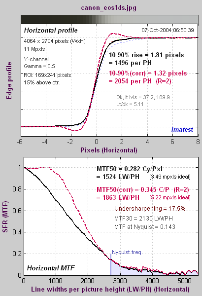
|
An undersharpened image
The 11 megapixel Canon
EOS-1Ds DSLR
is unusual in that it has very little built-in sharpening (at least in this particular sample).
The average edge (with no overshoot)
is shown on top; the MTF response is shown on bottom. The black
curves are the original, uncorrected data; the dashed red curves have standardized sharpening applied.
Standardized sharpening results in a small overshoot in the spatial
domain
edge response, about what would be expected in a properly sharpened
image. It is relatively consistent for all cameras. |
Oversharpening or undersharpening is the degree to which the uncorrected pulse is over- or undersharpened, i.e., sharpened relative to the standard sharpening
value.
It is equal to 100% (MTF( feql )-1). It if is negative (the
case for the EOS-1Ds), sharpening is applied to the original response;
if it is positive, de-sharpening is applied. (I use "de-sharpening"
instead
of "blurring" because the inverse of sharpening is, which applied here,
is slightly different from conventional blurring.) Note that it is not
the actual sharpening applied by the camera and software.
|
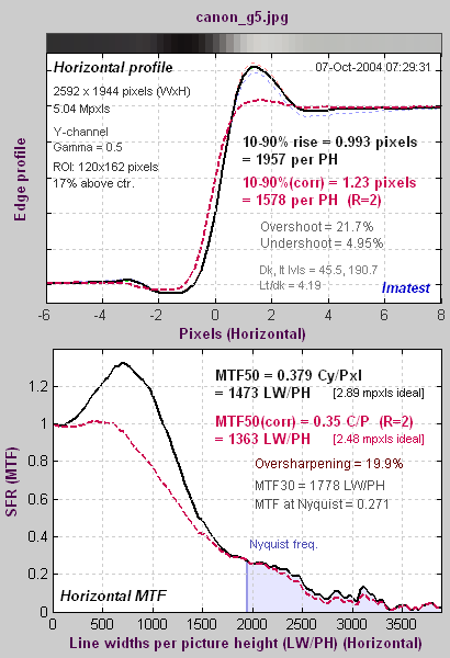
|
An oversharpened image
The image to the right is for the 5 megapixel Canon G5, which
strongly oversharpens the image— typical for a compact digital camera.
The uncorrected 10-90% edge rise distance of the G5 is
considerably
better than the 11 megapixel EOS-1Ds (1940 vs. 1511 per PH), but the
corrected
10-90% rise (with standard sharpening) is 76% of the EOS-1Ds. Based on
pixels alone, the expected percentage ratio would be 100% (1944/2704) =
72%.
MTF50P is not shown on the left. It is displayed when Standardized sharpening is turned off; it can also be selected as a Secondary readout (in place of MTF30 on the left). For this camera MTF50P is 345 cycles/pixel or 1340 LW/PH, almost 8% lower than MTF50. It's a slightly better sharpness indicator for strongly oversharpened cameras, especially in cases like video cameras where the image will not be post-processed.
|
The raw MTF50 of the G5 is close to the EOS-1Ds, but the corrected
MTF50
(with standard sharpening) is 73% of the EOS-1Ds, very close to the
ratio
of vertical pixels.
These results illustrate how uncorrected rise distance and MTF50
can
be misleading when comparing cameras with different pixel
sizes
and degrees of sharpening. MTF50P is slightly better for comparing cameras when strong sharpening is involved.
Uncorrected MTF50 is, however, appropriate
when
comparing lens performance (different focal lengths, apertures, etc.) on a single
camera.
Unsharp masking
"Unsharp masking" (USM) and "sharpening" are often used interchangeably, even though their mathematical algorithms are different. The confusion is understandable and far from serious because the end results are visually similar. But when sharpening is analyzed in depth the differences become significant.
"Unsharp masking" derives from the old days of film when a mask for a slide, i.e., positive transparency, was created by exposing the image on negative film slightly out of focus. The next generation of slide or print was made from a sandwich of the original transparency and the fuzzy mask. This mask served two purposes.
- It reduced the overall image contrast of the image, which was often necessary to get a good print.
- It sharpened the image by increasing contrast near edges relative to contrast at a distance from edges.
Unsharp masking was an exacting and tedious procedure which required precise processing and registration. But that has changed. USM can now be accomplished with only a few mouse clicks in an image editor.
Thanks to the
central limit theorem, blur can be expressed by the
Gaussian function (Bell curve).
Blur = exp(-
x2/2
σx2 ) / sqrt(2
πσx2 )
σx corresponds to the sharpening radius,
R. The unsharp masked image can be expressed as the original image summed with a constant times the
convolution of the original image and the blur function, where convolution is denoted by *.
LUSM(
x) =
L(
x) -
kUSM *
Blur
=
L(
x)
*
[δ(
x) -
kUSM exp(-
x2/2
σx2 ) / sqrt(2
πσx2 )] / (1-
kUSM /sqrt(2
π) )
L(
x) is the input pixel level and
LUSM(
x) is the USM-sharpened pixel level.
kUSM is the USM sharpening constant (related to the slider setting scanning or editing program).
L(x) = L(
x)
*
δ(
x), where
δ(
x) is a
delta function.
The USM algorithm has its own MTF (the
Fourier transform of the portion inside the brackets [...]).
Using
F(exp(-
px2) ) = exp(-α
2/4
p)/sqrt(2
p), where
F is the Fourier transform,
MTFUSM( f ) = [1- kUSM exp(-f 2σx2/2 ) /sqrt(2π) ] / (1- kUSM /sqrt(2π) )
= [1- kUSM exp(-f 2/ 2 fUSM2 ) /sqrt(2π) ] / (1- kUSM /sqrt(2π) )
where
fUSM = 1
/σx. This equation boosts response at high spatial frequencies, but unlike sharpening, response doesn't reach a peak then drop. Actual sharpening is a
two dimensional operation.
Future versions of Imatest may use USM for more highly optimized Standardized Sharpening algorithms.
Sharpness comparisons
for several digital cameras
Sharpness results derived from Websites
Several websites publish images of ISO 12233 test charts that can be entered into Imatest SFR to obtain detailed sharpness measurements. This page contains sharpness results derived from charts downloaded from two sites:
The measurements in the tables below come from two areas of the ISO 12233 image, illustrated by red rectangles in the image below.
- First row: near the center. The rectangle just above the center of the chart (about 15% of the distance to the corners).
- Second row: near the corner. The rectangle in the lower right of the chart (about 78% of the distance to the corner). Results include Chromatic aberration, which cannot be measured near the center.
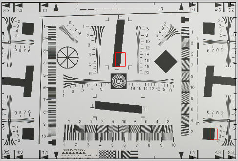
These measurements are limited to
- One lens. For DSLRs this is usually one of the sharpest available, such as the 50mm f/1.4 prime (non-zoom).
- One focal length. Sharpness is a strong function of focal length for zoom lenses. The sites aren't very consistent in their choice of focal length for zooms in compact digital cameras; long, short or intermediate focal lengths may be chosen.
- One aperture, typically around the optimum: f/8-f/11 for DSLRs; f/4-f/5.6 for compact digital cameras.
- One ISO speed, which strongly affects noise and dynamic range, but has little effect on sharpness.
- One sharpening radius, typically 2, used in standardized sharpening calculations, indicated by (corr.) and red columns.
- One or two vertical edges (in most cases), resulting in horizontal MTF measurements. Sometimes vertical MTF (from horizontal edges) is different.
- One RAW converter (usually the JPEG converter built into the camera) with one setting, usually the default. The choce of converter and sharpness setting has a strong effect on sharpness measurements.
- Gamma assumed to be 0.5, typical for digital cameras. A 10% gamma error results in about a 2.5% MTF50 error. Though gamma error is rarely severe, gamma should be measured with Stepchart or Colorcheck for greatest accuracy.
- Exposure and lighting are not always optimum. If the image is too dim or bright there may be some clipping on data (where it goes pure black or white), which reduces the accuracy of the sharpness measurement. Lighting may not be as even as it should be.
If you want to compare your own camera or lenses with the published charts, test lenses at various focal lengths and apertures, or observe the effects of ISO speed and signal processing, you'll need to download Imatest. The trial version allows up to twenty runs.
Explanation of results
| Megapixels |
The total megapixel count for the camera. |
| Picture
height
pixels |
The picture height of the camera. Important because sharpness is measured in units of Edge Rises or Line Widths per Picture Height. |
| Oversharpening % |
The amount of sharpening relative to standardized sharpening, which results in a modest amount of overshoot, similar to what you might get after manually sharpening the image. Undersharpening (as reported in Imatest SFR) is displayed here as a negative number. |
| 10-90%
rises per PH
(raw) |
The number of intervals per Picture Height where the average edge signal (with gamma removed) rises from 10% to 90% of its final value. The more the better, though aliasing can be a problem for extremely high values (significantly larger than the picture height), especially with Bayer sensors. See Understanding sharpness and SFR tour. |
| 10-90%
rises per PH (corr.) |
The number of 10% to 90% rise intervals per Picture height after standardized sharpening. This allows cameras with different degrees of sharpening to be compared on a (relatively) fair basis. A sharpening radius of 2 is assumed, unless indicated below. This radius works well for oversharpened compact digitals, but radius = 1, used by Imaging-resource.com, may be more appropriate for find DSLRs. |
MTF50
LW/PH
(raw) |
The spatial frequency where contrast drops to half its low frequency value. This is the best indicator of sharpness. See Understanding sharpness and SFR tour. |
MTF50
LW/PH
(corr.) |
MTF50 with standardized sharpening applied (corrected). MTF50 with standardized sharpening is best for comparing cameras with different amounts of sharpening; MTF50 without standardized sharpening (uncorrected) is best for testing and comparing lenses on a single camera model. See note on sharpening radius, two rows above. |
| Chromatic aberration (CA) |
A measure of "color fringing" near the edges of the images. Units are pixels. Tends to increase linearly with the distance from the center of the image. Under 0.5 pixels is insignificant. Over 1.5 is severe: quite visible in large prints. See Chromatic Aberration. An improved CA measurement, percentage of distance from the image center, is being implemented. |
Shannon
capacity
MB |
The information capacity of the image, based on sharpness (with standardized sharpnening) and noise. It correlates well with perceived image quality. But it should be interpreted with caution because it is strongly affected by signal processing, especially noise reduction. Best when used with RAW files. The number below is for a signal with the same contrast (100%) as the target (around 80:1). Shannon capacity is a relatively new measurement. We are still learning how to interpret it. |
| Comments |
Contains the source of the image (DPR or IR), and, if available, the focal length, aperture, and ISO speed. |
Tables of results
DSLRs: Digital SLRs, which take interchangeable lenses. Used by professionals and serious amateurs. Sensor size is at least 22 mm diagonal. Larger and heavier than the compact digital cameras, below. This table is more complete than the table for compact digitals because it's where my interest lies (and there are far too many compacts to keep up with). For each camera, the results in the upper and lower rows are for the image center and edge, respectively, as illustrated here.
Reminder: Remember the limitations listed above: one lens, one focal length, one aperture, one ISO speed, one RAW converter & settings (usually) built-in, one sharpening radius (2 unless otherwise indicated), etc., when interpreting these results. Also remember that several important image quality factors such as noise and dynamic range have been omitted.
| Camera |
Mega-
pixels |
Over-
sharp-
ening %
Center |
10-90%
rises/PH
(raw)
Ctr |
10-90%
rises/PH
(corr.)
Ctr
|
MTF50
LW/PH
(raw)
Ctr |
MTF50
LW/PH
(corr.)
Ctr
|
Chro-
matic
Aber-
ration
Ctr |
Shannon
capacity
MB
Ctr |
Comments |
Picture
height
pixels |
| Corner |
Cor |
Cor |
Cor |
Cor |
Cor |
Cor |
| Canon EOS-1D Mk II |
8.2 |
-15 |
1351 |
1741 |
1355 |
1559 |
— |
5.56 |
DPR. 50mm f/9 ISO 100. Very little built-in sharpening. Optimized for speed. Same pixel count as EOS-20D, but larger pixels. |
| 2336
| -21 |
1178 |
1589 |
1173 |
1443 |
0.40 |
4.99 |
| Canon EOS-1Ds |
11 |
-17 |
1509 |
2045 |
1521 |
1860 |
— |
7.11 |
DPR. 100mm f/9 ISO 100. 24x36 mm sensor. Little, if any, built-in sharpening. |
| 2704 |
-17 |
1485 |
2016 |
1519 |
1852 |
0.30 |
7.06 |
| Canon EOS-1Ds Mk II (DPR) |
16.7 |
-16 |
1919 |
2520 |
1922 |
2240 |
— |
11.0 |
DPR. 50mm f/9 ISO 100. 24x36 mm sensor. Little, if any, built-in sharpening. Sharpening radius = 2. |
| 3328 |
(Image cropped (1/4 area); corners unavailable.) |
| Canon EOS-1Ds Mk II (IR) |
Horiz. |
-39 |
1908 |
3310* |
1938 |
3084* |
— |
— |
IR review results are shown. 100mm f/5.6 ISO 100. Horiz. and Vert. refer to the MTF direction, not the edge. *Sharpening radius = 1 improves results. Similar to results from the DPR image with radius = 1. |
| Vert. |
-47 |
1559 |
3063* |
1630 |
2909* |
— |
— |
| Canon EOS-10D |
6.3 |
0 |
1419 |
1508 |
1332 |
1335 |
— |
4.02 |
DPR. 50mm f/9 ISO 100. Nearly identical to
the EOS-300D. Very good
13x19 inch prints. |
| 2048 |
-1 |
1410 |
1480 |
1331 |
1339 |
0.55 |
3.95 |
| Canon EOS-20D |
8.2 |
5 |
2017 |
1907 |
1758 |
1725 |
— |
6.13 |
DPR. 50mm f/9 ISO 100. Successor to the EOS-10D. Excellent 13x19 prints: slightly better than the 10D. |
| 2336 |
3 |
1807 |
1686 |
1603 |
1576 |
0.52 |
4.66 |
| Fuji S2 Pro |
6/12* |
-12 |
1869 |
2104 |
1819 |
1832 |
— |
7.19 |
DPR. 50mm f/9.5 ISO 100. *SuperCCD diagonal
pixel array. Uses interpolation to increase pixel count. Unusual ringing
in edge. High noise reduction? |
| 2848 |
-7 |
1699 |
1987 |
1708 |
1756 |
0.73 |
6.72 |
| Kodak SLR/c |
14 |
7 |
3571 |
3457 |
3184 |
3177 |
— |
15.1 |
DPR. 24x36 mm sensor. No anti-aliasing filter. (MTF > 0.5 at Nyquist.) Exceptional sharpness, but has problems with color Moire, illustrated
here.
Strong noise reduction. Discontinued. |
| 3000 |
(Image cropped (1/4 area); corners unavailable.) |
| Nikon D2X |
12.4 |
-5 |
2082 |
2382 |
2074 |
2098 |
— |
9.04 |
DPR. f/8 ISO 100. 23.7 x 15.7 mm sensor. |
| 2828 |
(Image cropped (1/4 area); corners unavailable.) |
| Nikon D100 |
6 |
-3 |
1381 |
1437 |
1243 |
1262 |
— |
3.44 |
DPR. 50mm f/'9. Competitive with the
Canon EOS-10D. |
| 2000 |
-4 |
1300 |
1373 |
1186 |
1227 |
0.74 |
3.3 |
| Nikon D70 |
6 |
5 |
1590 |
1897 |
1766 |
1759 |
— |
4.72 |
DPR. 50mm f/9. Weaker anti-aliasing
filter than the D100. Excellent sharpness for the pixel count. Relatively high MTF at Nyquist (0.4) could indicate Moire problems, but I've heard few complaints. |
| 2000 |
4 |
1769 |
1849 |
1700 |
1688 |
0.71 |
4.61 |
| Olympus E1 |
5 |
-8 |
1174 |
1351 |
1142 |
1215 |
— |
2.89 |
DPR. 50mm f/5 ISO 100. (Wider than optimum aperture) 4/3" format. Curious spikes in noise spectrum at quarter multiples of Nyquist. Otherwise relatively flat noise spectrum indicates little noise reduction. |
| 1920 |
-10 |
1121 |
1325 |
1105 |
1201 |
0.21 |
2.86 |
| Sigma SD10 |
3.4 |
-2 |
1574 |
1618 |
1508 |
1508 |
— |
3.53 |
DPR. 50mm f/9 ISO 100. Foveon sensor: no
Bayer array. No anti-aliasing filter. Outstanding sharpness for the number
of pixels (if only it had more!) Very high MTF at Nyquist
(0.5), but little apparent problem with Moire. See this Foveon report. |
| 1512 |
-2 |
1463 |
1487 |
1381 |
1383 |
1.0 |
3.18 |
Compact digital cameras: These are primarily consumer cameras, though many produce excellent image quality, especially for letter-size or A4 prints. Most have non-interchangeable zoom lenses. Maximum sensor size is 11 mm diagonal.
| Camera |
Mega-
pixels |
Over-
sharp-
ening %
Center |
10-90%
rises/PH
(raw)
Ctr |
10-90%
rises/PH
(corr.)
Ctr
|
MTF50
LW/PH
(raw)
Ctr |
MTF50
LW/PH
(corr.)
Ctr
|
Chro-
matic
Aber-
ration
Ctr |
Shannon
capacity
MB
Ctr |
Comments |
Picture
height
pixels |
| Corner |
Cor |
Cor |
Cor |
Cor |
Cor |
Cor |
| Canon G3 |
4 |
18 |
1636 |
1360 |
1265 |
1157 |
— |
2.19 |
DPR. 17.6mm f/4.5. Oversharpened. |
| 1704 |
11 |
1346 |
1186 |
1134 |
1052 |
1.27 |
|
| Canon G5 |
5 |
20 |
1931 |
1565 |
1458 |
1346 |
— |
2.88 |
DPR. 14.4mm f/4.0. Oversharpened. The chromatic aberration is not quite as bad as indicated because R and G are together; only B, to which the eye is less sensitive, is separate. |
| 1944 |
12 |
1774 |
1544 |
1399 |
1327 |
1.81 |
2.78 |
| Canon G6 |
7 |
12 |
2024 |
1780 |
1707 |
1612 |
— |
4.39 |
DPR. 15.2mm f/5.0. |
| 2304 |
-1 |
1738 |
1726 |
1599 |
1606 |
0.9 |
4.24 |
Fuji
F810 |
12.3* |
13 |
2085 |
1962 |
1944 |
1791 |
— |
6.02 |
DPR. 15.1mm f/5.6 ISO 80. *SuperCCD diagonal pixel array. Pixels are doubled in the test image. The lens is much better at the edges than the S7000. |
| 3040 |
-6 |
1906 |
1937 |
1829 |
1762 |
2.19 |
5.87 |
Fuji S7000
UL
LR |
6/12* |
22
|
2014
|
1853
|
1912
|
1625
|
—
|
5.21
|
DPR. 13mm f/5.6 ISO 200 (a high ISO speed for a compact; somewhat noisy). Oversharpened. *SuperCCD diagonal pixel array; 6 megapixels orig; 12 used for measurement. Uses interpolation to increase pixel count. UL = upper left; LR = lower right (the usual) ROIs. Softness on the left was noted by dpreview.com. Edge falloff is considerable. |
| 3040 |
-17
-22 |
1137
1202 |
1567
1591 |
1241
1230 |
1388
1446 |
2.67
2.04
|
4.52
4.62 |
| Fuji S9000 |
9.1 |
-3 |
2233 |
2534 |
2233 |
2242 |
— |
|
DPR. "Prosumer" 21 mm f/5.0 ISO 80. Impressive performer. |
| 2616 |
-13 |
1554 |
1979 |
1669 |
1814 |
0.41 |
7.49 |
Konica-Minolta
DiMAGE A2 |
8 |
8 |
1829 |
1696 |
1611 |
1537 |
— |
4.71 |
DPR. 13.3mm f/5.0 ISO 64. |
| 2448 |
-3 |
1500 |
1580 |
1403 |
1432 |
1.29 |
4.37 |
| Sony DSC-F828 |
8 |
9
|
1949
|
1751
|
1694
|
1617
|
—
|
4.69
|
DPR. 22.3mm f/5.0 ISO 64. 8 megapixel. Noisy at ISO speeds above 64. Superb lens. |
| 2448 |
5 |
1884 |
1763 |
1669 |
1627 |
0.11 |
4.65 |
Sony
DSC-P150 |
7 |
9 |
1696 |
1689 |
1622 |
1537 |
— |
4.37 |
DPR. 15.1mm f/8 ISO 100. Stopped down well beyond optimum aperture. |
| 2304 |
-8 |
1331 |
1504 |
1340 |
1427 |
1.9 |
3.95 |
Interpretation of MTF50
What MTF50 do you need? It depends on print size. If
you plan to print gigantic posters (20x30
inches or over), the more the merrier. All
the cameras in the above tables can make excellent 8.5x11
inch (letter-size; A4) prints. At that size the best of
them wouldn't look much better than the 4 megapixel Canon G3 (or
any other high quality 4 megapixel camera).
With fine lenses, careful
technique, and a little extra sharpening, my 6.3 megapixel Canon EOS-10D (corrected MTF50 = 1335 LW/PH) makes very good 12x18 inch prints. Prints are quite sharp from normal viewing distances, but
pixels are visible under a magnifier or loupe; the prints are not as
sharp as the Epson 2200 printer is capable of producing. Prints made with the EOS-20D (corrected MTF50 = 1581 LW/PH) are have a slight edge: I'd call them excellent.
Softness
or pixellation would be visible on 16x24
inch prints made from the EOS-10D. The EOS-20D would perform slightly better, and several of the cameras listed in the table— especially the full frame (24x36mm sensor) DSLRs— perform even better.
The table below is an approximate guide to quality requirements. The equation for the left column is
| MTF50(Line Widths / inch on the print) = |
MTF50(LW/PH)
Print height in inches |
MTF50 in
Line Widths/inch
on the print |
Quality level— after post-processing, which may include some additional sharpening |
| 150 |
Excellent— Extremely sharp at any viewing distance. About as sharp as most inkjet printers can print. |
| 110 |
Very good— Large prints (A3 or 13x19 inch) look excellent, though they won't look perfect under a magnifier. Small prints still look very good. |
| 80 |
Good— Large prints look OK when viewed from normal distances, but somewhat soft when examined closely. Small prints look soft— adequate, perhaps, for the "average" consumer, but definitely not "crisp.". |
Example of using the table: My Canon EOS-10D has MTF50 = 1335 LW/PH (corrected; with standardized sharpening). When I make a 12.3 inch high print on 13x19 inch paper, MTF50 is 1335/12.3 = 108 LW/in: "very good" quality; fine for a print that size. Prints look excellent at normal viewing distances for a print this size.
This approach is more accurate than tables based on pixel count (PPI) alone. Pixel count is scaled differently; the numbers are around double the MTF50 numbers. The EOS-10D has 2048/12.3 = 167 pixels per inch (PPI) at this magnification. This table should not be taken as gospel: itwas first published in October 2004, andit may be adjusted in the future.
Some observations
There has been a good deal of skepticism about
7+ megapixel compact digital cameras. They live up to
expectations for sharpness, but their noise may be objectionable
at high ISO speeds. Dpreview.com
has found the Sony DSC-828's noise
at ISO 64 to be as high as the Canon EOS-300D (similar to the EOS-10D)
at ISO 800.
The 6 megapixel raw/12 megapixel interpolated
Fuji S7000, which uses Fuji's SuperCCD, has sharpness comparable to the
Sony F828. It also has some problems with noise. The SuperCCD is based
on an interesting concept. Thanks to gravity, most detail in nature is
vertical or horizontal, and evolution has made our eyes are more sensitive
to those directions. SuperCCD pixels are located on a diagonal grid where
the spacing between x and y-pixel spacings is 1/sqrt(2) = 0.707 that of
a normal grid the same number of pixels. The diagonal grid is interpolated
to a horizontal grid that has twice the pixels, keeping the reduced pixel
spacing. This results in an impressive gain in horizontal and vertical
resolution, though sharpness is slightly below that of a sensor with the
same number of uninterpolated pixels.
I analyzed the sides of Fuji F7000 because dpreview.com
noted a problem with softness
on the left side. Uncorrected
MTF50 is the appropriate metric for comparing portions of a single image.
The problem is indeed very evident. It seems to be slightly worse on the
left, where MTF50 (uncorrected) is 62% of the center value.
The lens alsohas a problem with chromatic aberration. The Sony DSC-F828
does much better: edge MTF is 93% of the center value. It apears to have
a finer lens, at least at the focal length and aperture chosen for the
test.
The Sigma SD9 has high resolution for its pixel
count because it doesn't have, and probably doesn't need, an anti-aliasing
filter. If only Foveon could break the 3.4 megapixel barrier...
Links
Scanner Bake-off
2004 Jim Hutchinson used Imatest results in his comparison
of scanners.
Chromatic Aberration
AKA Color fringing
Introduction
Chromatic aberration (CA) is one of several aberrations that degrade
lens performance. (Others include coma, astigmatism, and curvature of
field.)
It occurs because the index of refraction of glass varies with the
wavelength
of light, i.e., glass bends different colors by different amounts. This
phenomenon is called dispersion.
Minimizing chromatic aberration is one of the goals of lens design. It
is accomplished by combining glass elements with different dispersion
properties.
But it remains a problem in several lens types, most notably ultrawide
lenses, long telephoto lenses, and extreme zooms.
Lateral and Longitudinal CA; Tangential and radial lines
Measurement tip— Lateral chromatic aberration is best measured using a tangential edge near the side or corner of the image, for example, B on the left. It is not visible on radial edges such as A.
CA cannot be measured reliably if the center of the region of interest (ROI) is less than 30% of the distance from the center to the corners. In this case, the chart will be displayed in pale colors and CA in % will be omitted. |
|
The two types of chromatic aberration are illustrated above.
-
Longitudinal chromatic aberration causes different
wavelengths to
focus on different image planes. It cannot be measured directly by
Imatest;
it causes a degradation of MTF response-- by differing amounts for
different
colors.
-
Lateral chromatic aberration is the color fringing
that occurs because
the magnification of the image differs with wavelength. It tends to be
far more visible than longitudinal CA. Imatest measures Lateral CA. A
software
technique for reducing with is described in Eliminating
chromatic aberration.
Lateral chromatic aberration is
best measured
on a tangential edge near the sides or corners of an image. It's
not
visible on radial edges. Radial lines and tangential curves (which differ by
90
degrees) are shown in burgundy and
blue
on the right side of the above illustration. Because Imatest SFR
requires
edges to have an angle in the range of 3 to 7 degrees with respect to
vertical
and horizontal, only a limited number of locations in the ISO 12233 chart (on the right) are appropriate for
measuring lateral CA. One is rectangle B,
above. SFR/SVG charts, which can be printed any size on high quality photographic inkjet printers, are much better for measuring CA.
The thumbnail on
the right is from a 12 megapixel compact digital camera with
fairly high chromatic aberration. The selected area is shown
below.
Red fringing, the result of lateral CA, is clearly visible. The
black-to-white
edge to the right side of this rectangle has equally vivid green
fringing.
Imatest analyzes the edge and produces a number that indicates the
severity
of the lateral chromatic aberration.
|
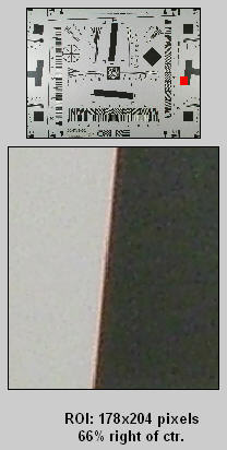
ROI for CA measurement |
Imatest chromatic aberration measurement
The average transitions for the R, G, and B color channels, calculated by
Imatest
SFR for the above edge, are shown in the figure below. The edges have been normalized to have asymptotic limits of 0 and 1, i.e., they are dimensionless, approaching 0 and 1 at large distances from the transition center. Note that the three edges are not simply shifted, as you might expect if the focal lengths for the three colors were slightly different. They are distorted due to demosaicing (RAW conversion), as discussed below. When Bayer RAW images are analyzed, you do indeed see simple shifts.
The visibility of the
chromatic
aberration is proportional to the area between the edges with highest
amplitude
(in this case, red) and
the lowest (in this case, blue). This area can be expressed by the following integral.
CA (area) = ∫ [ Smax(x) - Smin(x) ] dx
|
Since x has dimensions of distance in pixels and S is dimensionless, CA (area) has units of pixels— units of distance even though it is an area. CA defined by this equation is called the area
chromatic aberration. It is displayed in magenta in the figure on the right. (CA
(area)
= 1.92 pixels).
The distance between the crossings (the centers of the transitions) is also shown. It is less visually significant.
While area in pixels is a good measure of CA, it has some shortcomings.
- It penalizes cameras with high pixel counts.
- The result depends on the measurement location. The chromatic aberration in most lenses is roughly proportional to the distance from the image center.
|
Chromatic Aberration figure (relatively high CA)
(shown reversed: levels always increase from left to right) |
To deal with these issues Chromatic aberration is also measured in percentage of the distance from the image center to the corner (percentage of sensor diagonal/2) , corrected for the angle of the ROI with respect to the center. In the above example, CA (area) = 0.115% of the distance from the image center. The correction is described in the green box, below. This measurement gives the best overall results, since it's relatively independent of the measurement location and the number of pixels. A table below presents rough guidelines for the severity of CA. Measurements displayed on the right of the figure are summarized in the following table.
| 10-90% rise distance (original; uncorrected) in pixels and rises per picture height (PH). |
| CA (area): Chromatic aberration area in pixels. An indicator of the visibility of CA. The area between the channels with the highest and lowest levels. In units of pixels because the x-axis is in pixels and the y-axis is normalized to 1. Explained in the page on Chromatic aberration. Measured in along the axis indicated by Profile on the upper-left. Meaning (now obsolete): Under 0.5; insignificant. 0.5-1: minor; 1-1.5: moderate; 1.5 and over: serious. |
| CA (area) as a percentage of the distance to image center. A better indicator than pixels (above). Equal to 100 * (area between the channels with the highest and lowest levels) / (distance from center in pixels), corrected for the angle of the ROI. This number is relatively independent of the ROI because CA tends to be proportional to the distance from the image center. Explained in the page on Chromatic aberration. Measured along the radial line from the image center to the edge. Meaning: Under 0.04; insignificant. 0.04-0.08: minor; 0.08-0.15: moderate; over 0.15: serious. |
| CA (crossing). Chromatic aberration based on the most widely separated edge centers (positions where the edges cross 0.5). Tends to be less indicative of CA visibility than CA (area). Measured two ways: (A) in pixels along the axis indicated by Profile in the upper left, and (B) in percentage of the distance from the image center to corner along the line from the image center. |
| R-G, B-G Red−Green and Blue −Green crossing shift expressed as percentage of the distance from the image center to corner, measured along the radial line from the image center. R-G is r(R)-r(G), where r is radius in percentage of difference to the corner.. |
| R-G, B-G Red−Green and Blue −Green crossing shift expressed in pixels, measured along the axis indicated by Profile in the upper left. R-G is x(R)-x(G) for horizontal profiles or y(R)-y(G) for vertical profiles, where x and y are distances along the horizontal and vertical axes, respectively. The sign may be different from the sign in the percentage measurement, depending on the measurement quadrant. |
| Average pixel levels in the dark and light areas. Clipping can occur if they are too close to 0 or 255. |
Because Chromatic Aberration cannot be measured accurately near the image center, the chart is rendered in pale colors with the Region of Interest (ROI) is less than 30% of the distance from the center to the corner.
Severity
of chromatic aberration
Chromatic
Aberration
in percentage of
distance from
the image center |
Severity |
| 0-0.04 |
Insignificant |
| 0.04-0.08 |
Low. Hard to see
unless
you look for it. |
| 0.08-0.15 |
Moderate.
Somewhat visible
at high print magnifications. |
| over 0.15 |
Strong. Highly
visible at
high print magnifications. |
Severity
of chromatic aberration (old table)
Chromatic
Aberration
in pixels |
Severity |
| 0-0.5 |
Insignificant |
| 0.5-1 |
Low. Not visible
unless
you look for it. |
| 1-1.5 |
Moderate.
Somewhat visible
at high print magnifications. |
| over 1.5 |
Severe. Highly
visible at
high print magnifications. |
�
| Purple fringing
is not chromatic aberration, though it is often mistaken
for it. It's a saturation phenomenon in the sensor, also known as "bloom," caused by the
overflow
of electrons from highly saturated pixel sites to nearby unsaturated
sites.
It tends to be worst in cameras with tiny pixels (e.g., 8+ megapixel
compact
digital cameras). It has everything to do with the sensor and nothing
to
do with the lens. |
Demosaicing
Demosaicing is the process of converting Bayer RAW images, which have one color per pixel (RGRGRG...; GBGBGB...), to standard images, which have three colors per pixel. In the process of demosaicing, missing detail for each channel is inferred from detail in other channels. This is especially significant for Red and Blue pixels, which are half as common as Green. Demosaicing algorithms can be very mathematically sophisticated, but all of them can perform poorly in the presence of lateral CA, where detail is shifted from its expected location.
Demosaicing explains the shifted edges shown in the above example. Lateral CA cannot be reliably corrected after demosaicing, but it can be corrected to near-perfection prior to demosaicing. Correction coefficients can be calculated with Imatest Master, which can analyze Bayer RAW files created by converting manufacturer's Camera RAW files. Details are in the page on RAW files.
Here is an example illustrating the same region for a RAW and demosaiced file. Canon EOS-20D, 17-85mm IS lens, 53mm, f/11.
Chromatic aberration before demosaicing: easy to correct using a different
magnification for each color ( (1-0.00023)x for red;
1.000622x for blue; 1 for green).
Chromatic aberration after demosaicing: difficult to correct.
R-G and B-G are the CA correction coefficients. They are the spacing between the Red and Green and Blue and Green crossings, respectively, expressed as percentage of the center-to-corner distance. This mesurement is relatively independent of the location of the measurement.
 Corrected chromatic aberration measurements
In Imatest, edge profiles are measured along horizontal or vertical lines. The blue line (x) on the right is an example. But chromatic aberration takes place along radial lines-- lines from the center of the image to the region of measurement (shown in red on the right). Unless this line is vertical or horizontal, there will be a measurement error that must be corrected. The correction is illustrated on the right for a near-vertical edge, where the profile, and hence CA, is measured horizontally. In this illustration,
- x = x1 + x2 is the measured chromatic aberration, along a horizontal row of pixels.
- C = the true chromatic aberration, along the radial line (angle = Θ ).
- Φ is the angle of the edge relative to vertical.
x1 = C cos Θ ; y = C sin Θ ;
x2 = y tan Φ ( x2 may be negative if Φ is negative.)
x = x1 + x2 = C cos Θ + y tan Φ = C ( cos Θ + sin Θ tan Φ )
C = x / ( cos Θ + sin Θ tan Φ )
Veiling glare (Lens flare)
Veiling glare is stray light in lenses and optical systems caused by reflections between surfaces of lens elements and the inside barrel of the lens. It is a strong predictor of lens flare— image fogging (loss of shadow detail and color) as well as "ghost" images— that can degrade image quality in the presence of bright light sources in or near the field of view. It occurs in every optical system, including the human eye.
Lenses with low flare have been traditionally known for their excellent color performance. Color saturation is higher, especially in shadows. Low flare may be as responsible as sharpness for the exalted reputations of some classic Leica and Zeiss lenses. Even though lost color saturation and contrast can be recovered with digital processing, lenses with low flare will always have an edge in quality. There are several ways of dealing with lens flare.
- In lens design, veiling glare is controlled by using high quality lens coatings (multiple coatings are best), baffling in the lens barrel, and careful design.
- In the field it is controlled by lens hoods and anything that can shield the lens surface from the sun. Ansel Adams used his hat, as well as a bellows lens shade, made famous in a Datsun (Nissan) commercial.
- In the studio it is controlled by "barn doors" on light sources.
 |
 |
Obligatory bad photo showing
severe lens flare caused by the sun (far left), and
moderate flare with the sun blocked (near left).
Canon EOS-20D, 24-70mm f/2.8L, 24mm, f/8, no hood.
Taken during Colorado's notorious "Winter of 2007"
(five feet of snow in three weeks in December and January)
The veiling glare measurement in Imatest Stepchart is designed to give a good prediction of a lens's susceptibility to lens flare in challenging situations: the larger the number, the worse it's likely to be. But it's not perfect in every detail. For example, it can't predict ghosting (visible behind the Stop sign in the image on the left).
The measurement is fairly simple to perform, but several pitfalls can cause inaccurate or misleading results unless measurements are made with care. Some degree of exposure control— either a manual setting or exposure compensation— can enhance the accuracy of the results. Exposure may be a problem with cameraphones and other simple devices, where little, if any, control is available. |
Veiling glare is measured by photographing a perfectly black object against a uniform white field that extends well beyond the image frame. It is defined as the ratio of the light reaching the sensor from the black object (which emits no light) to the light reaching the sensor from the surrounding white field.
|
 |
Veiling glare = V = L(black object) / L(white surface), where L is the illuminance at the sensor.
Since digital image sensor output is linear, this measurement is straightforward
- if you have access to the linear (RAW) output of the sensor,
- if the white area is unsaturated,
- if the signal in the black area is large enough to be well above the noise, and
- if the black area is perfectly black.
We deal with the last of these issues first: how to create a perfectly black object— a black hole. Don't worry: it's more environmentally friendly than the type that sucks entire planets into its core.
Preparing the target
The black hole
The darkest surfaces— materials or pigments— reflect about 0.5 to 1% of the incident light, i.e., they are are far from perfectly black. To obtain a surface suitable for measuring veiling glare you will need to construct a surface that little light reaches— a black hole— the darkest possible object that can be photographed in a bright environment.
The black hole should be constructed inside a box or tube that is approximately 3x4 inches on its top (or 4 inches in diameter) and 4-8 inches deep. The bottom (inside back surface) should be lined with black velvet— the darkest material you can buy. The sides can be lined with any matte black material. We used black art paper because it was easy to work with. The top is a piece of black foam board with a 1x2 inch opening cut in the center.
The structure should be kept as lightweight as possible. If necessary it can be constructed entirely out of black foam board, with the black velvet in the inside back surface. |
Construction of the "black hole" |
The black hole is mounted next to a standard step chart such as the Kodak Q-13 or Q-14, which performs two functions. It allows you to measure the camera's tonal response (pixel level as a function of scene luminance) and it provides a reference for determining the white level from a deep gray patch, so you don't have to measure it directly. This is important because many, if not most cameras, have nonlinear response in the bright regions, i.e., the response curve has a (film-like) "shoulder"— a good thing pictorially because without it digital cameras have a strong tendency to burn out highlights.
An alternative: Bart van der Wolf sent this link, which suggests that a cone painted glossy black can be used to make a superior black hole.
Gamma (image contrast) for measuring veiling glare is calculated somewhat differently from the average gamma shown in the figures. It is determined from the region where the step chart pixel level is between 0.1 and 0.6 of the minimum-to-maximum pixel range, i.e., the brightest areas, which are frequently nonlinear in digital cameras, are excluded. The white reference is inferred from the patch in the middle of this region. For example, suppose it is patch 11. Since the Q-13/Q-14 has density steps of 0.1, patch 11 is 1.0 density units darker than (1/10 as bright as) patch 1, which is the reference white, i.e., we infer the white level from the measurement of patch 11: the inferred white pixel level would be (10 times the pixel level of patch 11)gamma. Since nonlinearity or even clipping of highlights is quite common, this technique results in a much more accurate veiling glare measurement than you'd get by measuring the white region directly. Tonal response for an in-camera JPEG and a linear (simple gamma curve) RAW conversion are shown here. Here is the modified veiling glare equation.
Veiling glare = V = ( Pixel level (black object) /Pixel level (white surface, inferred) )1/gamma
Assembling the target
A Kodak Q-13 step chart and the black hole box are mounted on a piece of mat board, roughly twice the width of the Q-13 chart— its dimensions are not critical. A 3/4x1 inch hole is cut in the mat board, just to the right of where of where the Q-13 chart will be mounted. The black hole box is mounted behind it. The Q-13 is mounted to slightly overlap the opening. The mat board is attached to the 40x60 inch white foam board with Velcro so it can be easily removed for safe storage.
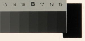 |
Black hole
location
detail |
|
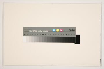
Typical framing for measurements |
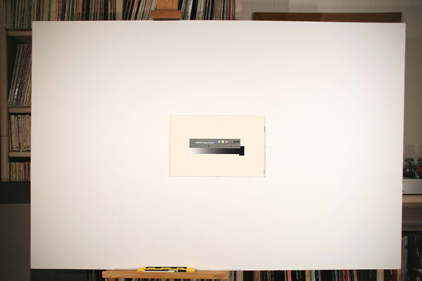
The entire target
Measuring veiling glare
- Illuminate the target evenly, with no more than about ±20% variation in illumination across the target, as described in Imatest test lab. Keep the ambient light near the camera as low as possible ti minimize the light entering the "black hole."
- Note whether you are using a lens hood or a filter (like the ubiquitous UV filter most photographers leave on their lenses for protection). Both affect veiling glare.
- Set the camera to the lowest available ISO speed to minimize the noise in dark patches.
- Adjust the exposure (or exposure compensation) so the white level is close to saturation, i.e., bias it in the direction of overexposure. It doesn't hurt if some highlights are blown out: the Imatest veiling glare algorithm is insensitive to highlight saturation.
- RAW output is preferred, though JPEG may be perfectly fine if the response is reasonably linear.
- Photograph the central portion of the target, leaving some white area around the Q-13 chart and "black hole." Typical framing is shown above, to the right of Assembling the target. The length of the white target to the left and right of the frame should be about equal the frame itself. Similarly, the length of the white target above and below the frame should be about equal to the frame itself. (Light entering the lens from outside the image frame is an important contributor to lens flare.)
- Run Imatest and select Stepchart. Open the image file. If Automatic Zone detection is unchecked and the image is the same size as the previous run you'll be asked if you want to repeat the same ROIs (Regions of Interest). If you enter No, you'll be asked to make an ROI selection. It's OK to make a rough selection: another window will enable you to refine it. After you've made the rough selection, the Stepchart input dialog box, shown below, appears. To measure veiling glare, Automatic Zone detection must be unchecked, Veiling glare must be checked, and the number of patches must be set to one greater than the number of patches in the step chart: 21 in this case.
Stepchart input dialog box, set for veiling glare
- Click OK. The fine adjustment box appears. Press Lighten, just to the right of Zoom out to view the dark patches clearly. The Lighten button changes to Normal when the image is in lightened mode. It also helps to maximize the window and click the Coarse radio button (middle, left).
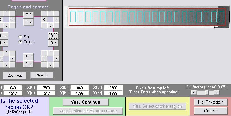
Portion of Fine ROI adjustment window; Lightened view ( Normal box is displayed)
- Click Yes, Continue to run Stepchart and calculate veiling glare.
Results
The first illustration shows the results for the Canon EOS-20D with the 24-70mm f/2.8L lens set at 70mm, f/8. Veiling glare is shown on the middle-right of the first figure.
with UV filter (not multicoated)
No filter: 23% lower veiling glare |
Overexposed about 2 f-stops, with UV filter:
Results are insensitive to overexposure. |
These plots show the difference in linearity between JPEG and RAW (to TIFF) density response. The EOS-20D only deviates slightly from linearity (a straight gamma curve).
JPEG density response,
showing nonlinearity in highlights
|
RAW/TIFF density response,
showing good linearity in highlights
|
Table of results: Canon EOS-20D JPEG data |
| Lens |
Elements |
Groups |
Focal length |
f-stop |
Veiling glare |
Comments |
| Canon 24-70mm f/2.8L USM (no hood; single-coated UV filter) |
16 |
13 |
70 |
8 |
0.453% |
A premium zoom, known for excellent sharpness. Results are strongly affected by the single-coated UV filter, but they are insensitive to overexposure. When working from RAW (CR2) images, veiling glare was 0.564% with the filter and 0.391% with without it. Different results; similar trends. |
| '' (no filter) |
0.348% |
| '' (overexposed 2 stops, with filter) |
0.464% |
| Canon 90mm f/2.8 TS-E (no filter) |
6 |
5 |
90 |
8 |
0.291% |
A very high quality tilt/shift lens with relatively few elements and groups. Has beautiful tonality and color quality. Low veiling glare expected. |
| Sigma 18-125mm f/2.5-5.6 DC (hood, multi-coated UV filter) |
15 |
14 |
77 |
8 |
0.293% |
A remarkably fine lens for the price. Surprisingly low veiling glare. (If you're thinking of buying one: it has poor autofocus performance; it's much better on manual.) |
| Canon 28-80mm f/3.5-5/6 (no filter) |
10 |
9 |
80 |
8 |
0.634% |
(1991 version) A cheap "kit" lens, designed for low cost. Expectations were low. Strangely reddish white balance. |
| Canon 70-200mm f/4L USM (UV filter, hood) |
16 |
13 |
70 |
8 |
0.396% |
Excellent lightweight lens. The IS version has 20 elements in 15 groups, which will increase flare. |
| The table at the bottom shows the relationship between the number of groups (sets of attached elements) and the number of reflections that contribute to veiling glare. |
Most of the results are not surprizing. The Canon 90mm has the lowest flare, while the cheap Canon 28-80 is the worst. The only surprise is the excellent performance of the Sigma 18-125: a lens know for its fine performance and value, though its autofocus performance is mediocre. I use mine on manual.
Limitations
The veiling glare may be underestimated for telephoto lenses— especially if they are measured without lens hoods— because telephoto lenses form an image of only a small fraction of the light reaching the front element (the portion is much larger with normal and wide angle lenses). The target, as shown above, may not be large enough to simulate all the light that reaches the lens. If a hood is used, this error is considerably reduced.
If there are nonlinearities in the camera response at low light levels, the results may be incorrect (although relative results, i.e., comparisons, will still be valid). It's always safest to work with RAW images and convert them with a "linear" (i.e., simple gamma curve) setting. You can read many RAW formats into Imatest, using the dcraw converter.
Lens elements, groups, reflections, and flare— some geeky math fun
Lens flare is closely related to the number of secondary reflections in a lens, i.e., light entering the lens that is reflected off one lens surface, then another, then back to the image plane. For uncoated air-to-glass surfaces, about 4% of the incident light is reflected. Simple coating reduces the reflection to around 2%; muti-coating reduces it to 1% or less. For a simple coating, the amount of the secondary reflection is 0.02 * 0.02 = 0.0004, which doesn't seem like much until you calculate the number of reflections.
A lens consists of N elements in M groups, where a group may consist of several elements cemented together. It's the number of groups M— actually the number of air-to-glass surfaces 2M— that really counts. The first surface has no secondary reflection. The second surface has 1: light that bounces off the second surface, then the first, then back to the image plane. Continuing with this reasoning, we see that the m(th) surface has m-1 secondary reflections, i.e.,
Total reflections = R = (2M-1) + (2M-2) + (2M-3) + ... + 1 = M (2M-1) = 2M2-M
If you add a filter to a lens with M groups, you increase the number of reflections R by 4M+1.
|
Groups
M
1
2
3
4
5
6
7
8
9
10
11
12
13
14 |
Reflec-
tions R
1
6
15
28
45
66
91
120
153
190
231
276
325
378
|
| Zooms typically have more elements than primes. Examples (easy to locate in the Canon Museum): The Canon 24-105mm f/4L IS USM has 18 elements in 13 groups. The Canon 50mm f/1.4 USM has 7 elements in 6 groups. The Canon 90mm f/2.8 TS-E has 6 elements in 5 groups. Now you know one reason primes are still used (others are large apertures, light weight, and excellent sharpness (MTF)), as well as why some photographers avoid using filters (though a UV filter is useful protection for field work). |
|
Color correction matrix
Introduction
Starting with Imatest 2.4.1, Multicharts can calculate a color correction matrix that can be applied to images to achieve optimum color balance, as defined by minimizing a color error parameter on the test chart of choice. (The default is the mean of (Delta-E 94)2 for all patches where L*>10 and L*<95.) The matrix can be used by imaging system designers in their cameras or image processing algorithms. For example, Micron sensors use a 3x3 correction matrix.
Some of the background for the calculation can be found in Color Correction Matrix for Digital Still and Video Imaging Systems by Stephen Wolf, though the Imatest calculation differs in many respects: there is no issue with outliers and optimization is performed using one of the standard color difference metrics.
The color correction matrix is initially included only in Multicharts. In the future it may be added to Colorcheck and additional linearization options will be offered.
The Math
The matrix
Color images are stored in m x n x 3 arrays (m rows (height) x n columns (width) x 3 colors). For the sake of simplicity, we transform the color image to a k x 3 array, where k = m x n. An Original (uncorrected) array O can be represented as
          | O_R1 O_G1 O_B1 |

      O = | O_R2 O_G2 O_B2 |

          |      ...       |
          |      ...       |
          | O_Rk O_Gk O_Bk |
where
O_Ri, O_Gi, and O_Bi represent the normalized R, G, and B levels of pixel i. The transformed (corrected) array is called P, where
P = O A (case 1: A is a 3x3 matrix) — or —
P = [O 1] A (case 2: A is a 4x3 matrix; the added column of 1s provides a dc-offset)
A is the 3x3 or 4x3 color correction matrix. For the 3x3 matrix,
          | P_R1 P_G1 P_B1 |    | O_R1 O_G1 O_B1 |

      P = | P_R2 P_G2 P_B2 | =  | O_R2 O_G2 O_B2 |   | A11 A12 A13 |

          |      ...       |    |      ...       | X | A21 A22 A23 |
          |      ...       |    |      ...       |   | A31 A32 A33 |
          | P_Rk P_Gk P_Bk |    | O_Rk O_Gk O_Bk |
X denotes matrix multiplication. In this case, for row m,
P_Rm = O_Rm*A11 + O_Gm*A21 + O_Bm*A31 (* denotes multiplication.)
P_Gm = O_Rm*A12 + O_Gm*A22 + O_Bm*A32
P_Bm = O_Rm*A13 + O_Gm*A23 + O_Bm*A33
For the 4x3 matrix, a column of 1s is added to provide a dc-offset,
          | P_R1 P_G1 P_B1 |    | O_R1 O_G1 O_B1 1 |   | A11 A12 A13 |

      P = | P_R2 P_G2 P_B2 | =  | O_R2 O_G2 O_B2 1 |   | A21 A22 A23 |

          |      ...       |    |       ...        | X | A31 A32 A33 |
          |      ...       |    |       ...        |   | A41 A42 A43 |
          | P_Rk P_Gk P_Bk |    | O_Rk O_Gk O_Bk 1 |
In this case, for row m,
P_Rm = O_Rm*A11 + O_Gm*A21 + O_Bm*A31 + A41
P_Gm = O_Rm*A12 + O_Gm*A22 + O_Bm*A32 + A42
P_Bm = O_Rm*A13 + O_Gm*A23 + O_Bm*A33 + A43
The goal of the calculation is to minimize the difference (the mean square error metric) between P and the reference array (the ideal chart values) R. The initial values of A (the starting point for optimization) for the 3x3 and 4x3 cases, are
               | k_R 0  0  |               | k_R 0  0  |

      A(3x3) = |  0 k_G 0  | ;   A(4x3) =  |  0 k_G 0  |

               |  0  0 k_B |               |  0  0 k_B |
                                           |  0  0  0  |
where
k_R = mean(R_Ri ; all i)/mean(O_Ri ; all i) for reference array R and original array O
k_G = mean(R_Gi ; all i)/mean(O_Gi ; all i)
k_B = mean(R_Bi ; all i)/mean(O_Bi ; all i)
These starting values are closer to the final values (have less mean square error) than the identity matrix (k_R = k_G = k_B = 1). They tend to converge slightly better.
Linearization
Although most digital image sensors are linear up to the point where they saturate, image files are highly nonlinear— they are designed for display at a specified gamma ( γ ), where display luminance = pixel levelγ. Gamma = 2.2 for the most commonly used color spaces (sRGB, Adobe RGB (1998) and Wide Gamut RGB (WGRGB)), although some well-known color spaces are designed for display at gamma = 1.8 (ProPhoto, Apply, ColorMatch; all RGB).
When cameras encode images (a part of the RAW conversion process), they apply a gamma that is the approximate inverse of the display gamma. Perhaps we should say very approximate: it may vary considerably from 1/γ, and it often includes a tonal response curve "shoulder" (an area of reduced contrast) to minimize highlight burnout. The shoulder makes the response more "film-like," improving pictorial quality in most instances.
The response should be linearized prior to applying the correction matrix, (though Imatest has the option of omitting linearization).
Optimization steps
- Linearize the input image (optional). If Color space gamma linearization is selected, OL = Oγ.
- Call the optimizer, which
- calculates a (temporary) corrected image TL = OL A.
- Remove the linearization: T = TL(1/γ)
- Finds the mean of squares of errors between T and the reference (ideal) array R. The error is one of the standard error measurements: ΔE*ab, ΔC*ab, ΔE94, ΔE94, ΔECMC, ΔCCMC, ΔE00, or ΔC00, described here. ΔE94 is the recommended default. Although the CIEDE2000 color error metrics (ΔE00, ...) are more accurate, they contain small discontinuities that can affect optimization, and hence they should be used with caution. See Sharma for details. The ΔC errors are similar to ΔE with luminance (L*) omitted.
- Adjusts A until a minimum value of the sum of squares of the errors is found, using nonlinear optimization.
- Report the final value of A.
In applying A (generally outside of Imatest), a similar linearization should be used. A may be applied during the RAW conversion process, prior to the application of the gama + tonal response curve.
There is no guarantee that A is a global minimum. Its final value depends to some extent on its starting value.
The Color correction matrix in Multicharts
Options:  Color matrix calculation options can be set by clicking Settings, Color matrix in the Multicharts window. This brings up the dialog box shown on the right. The options are
- 4x3 or 3x3 matrix: Color correction matrix size. The 4x3 matrix (the default) includes a dc-offset (constant) term. It may be slightly more accurate, but it takes more computation time.
- Optimize: Select the color error parameter whose mean of squares over patches with L*>10 (nearly black; color is invisible) and L*<95 (little chroma) is to be minimized. Choices include ΔE ab, ΔC ab, ΔE 94, ΔE 94, ΔE CMC, ΔC CMC, ΔE 00, and ΔC 00, described here. ΔE 94 is the default value, recommended because it gives less weight to chroma differences between highly chromatic (saturated; large a*2 + b*2 ) colors, which is closer to the eye's perception than ΔE ab (the standard ΔE value: the geometrical distance between colors in L*a*b* space).
- Weighting: Set the weighting of the patches for optimization. Choices:
- Equal weighting [default] Patches are equally weighted. May not be the optimum setting because highlight colors may be more visually prominent than shadow colors.
- Emphasize highlights: weight according to CIELAB L* Give more weight to visually-prominent hightlight patches.
- Strongly emphasize highlights: weight according to L*^2.
- Linearization: Choose the method of linearizing the image (or leave it unchanged). For linearization or gamma encoding, the value of gamma ( γ ) for the selected color space (sRGB, Adobe RGB, etc.) is used. The equation for linearization is OL = O1/γ. The equation for gamma application O = OLγ.
- Linearize input, apply matrix, then apply gamma encoding. This is the best choice for images encoded in a standard color space.
- No linearization: apply matrix to input pixels. Not generally a good choice for gamma-encoded images, but useful for experimentation and for images that start and remain linear.
- Assume linear input, apply matrix, then apply gamma encoding. A good choice for images that are not gamma-encoded, but need to be converted into a color space..
To calculate the color correction matrix, read the image into Multicharts, then press the Correction matrix button, shown on the right. The display will change, as shown below. The improvement for this image, which is quite good to begin with, is undramatic. |
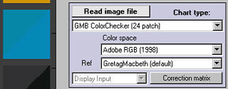 |
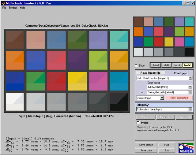
Split view, showing reference, input, and corrected patch colors
The image now shows the corrected colors on the bottom of each patch. The ideal (reference) color remains in the upper-left and the input (original) color remains in the upper right.
The Correction matrix button changes to Matrix calculated, highlighted with a pink background. The correction matrix cannot be recalculated until an image property changes (new image, color space, reference file, or color matrix setting). The Display input (or Corrected) dropdown menu, immediately to its left, is enabled. You can choose one of two selections.
| Display input |
Color differences (input − ideal) are shown in most displays, and [Input − ideal] Color differences are shown in the text in the lower left. Two displays are unaffected by this setting: Pseudocolor color difference and Split colors, where (corrected − ideal) is shown on the bottom. |
| Display corrected |
Color differences (corrected − ideal) are shown in most displays, and [Corrected − ideal] Color differences are shown in the text in the lower left. |
The EXIF data and Color matrix display has a summary of results.
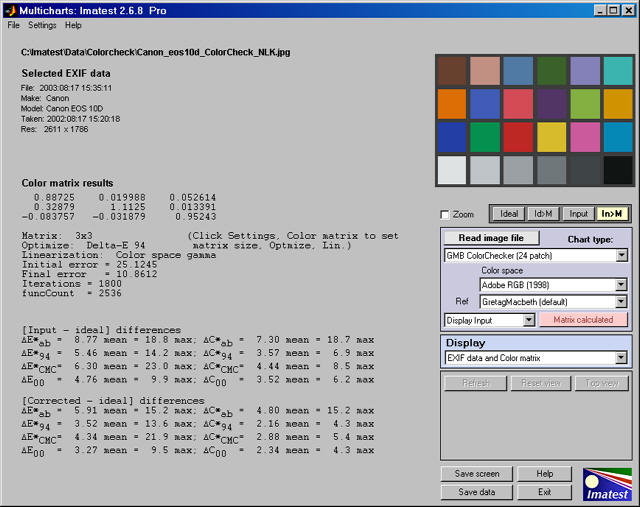
Exif and Color matrix view
The color correct matrix, results summary, and both [input - ideal] and [corrected -ideal] color difference summaries are shown. The initial and final error numbers shows how much the selected metric (in this case the sum of squares of Delta-E 94 for all patches with L*>10 and L*<95) has changed.
Blur units, MTF, and DXO Analyzer's BxU
Blur operations, MTF, and DxO®
Analyzer's BxU®*
In early 2004, DxO
Labs of Boulogne, France introduced a program for analyzing digital
image quality called DxO
analyzer®. It has aroused a great deal of interest,
but its price is far beyond the
means
of most photographers. (If you have to ask...) Several publications,
including
Luminous-landscape.com,
pictchallenge.com
(web), and France's outstanding Chasseur
d'Images (print) use it for testing cameras and lenses.
DxO analyzer measures sharpness using the Blur
Experience Unit (BxU®), which was defined by Luc Marin of DxO in a PMA 2005 PowerPoint presentation.
"Our convention : BxU = -1 for “Adobe PhotoShop 7.0” sharpen function.
Therefore “Sharpen more” BxU = -2.7"
It may seem counterintuitive to define blur in terms of sharpening (yes, it's confusing), but there's a reason: familiarity. Photographers rarely apply blurs, but sharpening is an important part of digital image processing. For best results sharpening needs to be applied to nearly every digital image (in the camera, RAW converter, and/or image editor).
In a conversation in late 2006, Dr. Frederic Guichard of DxO indicated that the BxU is proportional to the variance (σ2) of the line spread function LSF— the derivative of the average pulse— a convenient measurement that does not require an MTF calculation. Variance is displayed by Imatest SFR when Line spread function is selected for the Edge plot (the upper plot of the MTF figure).
In this page we derive an approximate relationship between BxU, MTF, and variance. We present it here, before we get into the details, which most readers will prefer to skip.
One BxU (DxO's Blur Experience Unit) is equivalent to 1 (or perhaps 1.25) applications of the Photoshop Blur filter.
Approximately (using 1 Bxu = 1 Blur),
MTF @ 0.25 cycles/pixel (half-Nyquist) = 0.862 * 0.78BxU).
MTF50 (cycles/pixel) = 1 / sqrt(6.067 BxU + 3.6)
These numbers were derived from the tables below using the observations that Blur is the approximate inverse of Sharpen and that the number of Blur applications is proportional to 1/MTF502. Alternatively,
BxU is approximately equal to 4.6 * LSF variance (σ2) in pixels |
The details
In the paper, "Uniqueness of blur
measure"
by
Jerome Buzzi
and Frederic Guichard, IEEE International Conference on Image
Processing,
2004 (which contains some truly formidable math), blur is is equated
with
the variance (σ
2 ) of gaussian blur, exp(-x
2
/
(2σ
2 )). (This one dimensional equation is somewhat simplified. DxO uses two-dimensions:
Blur = (σ
xx2
+ σ
yy2) / 2 ). Since σ has units of distance, this suggests that BxU is
proportional
to the square of the 10-90% rise distance.
And since the Fourier transform of a gaussian is itself a gaussian,
this
implies that
BxU is proportional to 1/MTF502. We examine this hypothesis below.
|
The effects of the Photoshop
6 Blur More and Blur filters were analyzed by applying each operation
five
times to an ideal edge of moderate contrast (pixel levels 202 and 50),
shown on the right unmagnified and magnified 4x.
The image on the lower right is the edge after two Blur Mores. Imatest
SFR produced the following MTF results.
| |
Blur more |
Blur |
| N |
MTF50
(C/P) |
m1 |
m2 |
R10-90
Pixels |
R10-
902 |
MTF @
.25 c/p |
σ2
Pixels |
MTF50
(C/P) |
m1 |
m3 |
MTF @
.25 c/p |
σ2
Pixels |
| 0 |
0.526 |
3.61 |
0 |
0.953 |
0.91 |
0.862 |
0.121 |
0.526 |
3.61 |
0 |
0.862 |
0.121 |
| 1 |
0.229 |
19.1 |
1.07 |
2.13 |
4.54 |
0.431 |
0.637 |
0.332 |
9.07 |
0.90 |
0.665 |
0.343 |
| 2 |
0.173 |
33.4 |
2.05 |
2.78 |
7.73 |
0.224 |
1.14 |
0.256 |
15.3 |
1.93 |
0.516 |
0.565 |
| 3 |
0.145 |
47.5 |
3.02 |
3.36 |
11.3 |
0.123 |
1.65 |
0.216 |
21.4 |
2.93 |
0.402 |
0.777 |
| 4 |
0.127 |
62.0 |
4.02 |
3.80 |
14.4 |
0.071 |
2.16 |
0.191 |
27.4 |
3.86 |
0.313 |
0.99 |
| 5 |
0.115 |
75.6 |
4.96 |
4.18 |
17.5 |
0.043 |
2.65 |
0.172 |
33.8 |
4.98 |
0.247 |
1.21 |
N = number of applications.
m1 = 1/ MTF502
Blur more: m2 = (m1-3.6)/14.52
Blur: m3 = (m1-3.6)/6.067
|
| Ideal edge |
| |
|
| Edge with Blur More applied twice |
 |
 |
| Unmagnified |
4X Magnified |
|
|
These results confirm an inverse square relationship between MTF50 and the number of Blur More and Blur applications. Two Blur more operations equals five Blur operations. m2 and m3 are approximately equal to the number of applications.
| |
Each application of
Blur More cuts the response at 0.25
cycles per pixel (half the Nyquist
frequency) by half. This suggests an equation (though probably not
the one used to calculate BxU): BxU = -log 2( MH)
= -3.322 * log 10( MH), where MH
is the MTF at 0.25 cycles per pixels (half-Nyquist).
|
The calculation of variance σ
2 is somewhat tricky. The equation is derived from probability theory, but it can behave strangely. σ
2 can have negative values because the line spread function
LSF(
t), which is the derivative of the averaged pulse, can have negative values (undershoots) that never occur for probability density functions.
First, the mean location of
LSF(
t) needs to be calculated. This can be done using
LSF or
LSF2. The latter seems to work better.
E(
t) = Σ
ti LSF2(
ti) / Σ
LSF2(
ti)
σ
2 = Σ (
ti-
E(
t))
2 LSF(
ti) / Σ
LSF(
ti)
The sum in the σ
2 equation has to be taken over a limited region so that noise at large distances from
E(
t) (i.e., outliers) does not distort the results. If
LSF2 had been used instead of
LSF in this equations, undershoots, which make edges look sharper, would
increase σ
2.
After we learned Luc Marin's definition of BxU = -1 for one Photoshop sharpen function, we ran some tests and found that the Sharpen function is the approximate inverse of the Blur function, at least when measured by MTF50. It's a little off when measured by MTF @ 0.25 cycles/pixel. The negative values of σ2 were caused by undershoots due to sharpening. |
|
| Test |
MTF50
(C/P) |
MTF @
0.25 cy/pxl |
σ2
Pixels |
| Original ideal edge |
0.526 |
0.862 |
0.121 |
| with one Blur |
0.332 |
0.665 |
0.343 |
| with one Sharpen |
0.753 |
1.28 |
-0.270 |
with one Blur + Sharpen
(order doesn't matter) |
0.531 |
0.973 |
-0.113 |
|
Pictchallenge.com adds a bit of confusion to the issue. Their extensive description of DxO states, "... une valeur de "2" correspond par rapport a cet ideal a un cran de "plus flou" de Photoshop." This appears to imply that 2 BxUs equals one Blur more, but I'm not certain— I'm not a master of French. They also have a DxO image that shows BxUs of around 1 for the outstanding Macro Nikkor 60mm lens. They translate BxUs into their own rating system, where sharpness (pique) of 3 is poor and 5 is excellent. I haven't been able to figure out the precise relationship between these numbers and BxU.
Since one application of Blur More is equal to 2.5 applications of Blur, Pictchallenge.com's statement implies that one BxU is equivalent to 1.25 Blur applications— a little confusing; 1 seems more likely.
Luminous-Landscape's erroneous BxU description
When we first became aware of DxO in July 2004, we struggled with an apparent discrepancy between published test results and Luminous-Landscape.com's definition of BxU as equivalent to one Blur More. Edge after Blur More has been applied 6 times. Unmagnified.
Reported BxU numbers appeared to be much too large to fit this definition. For example, Luminous-landscape.com, imaging-resource.com and dpreview.com tested the 8 megapixel Sony DSC-F828. The Imatest SFR analyses of the ISO-12233 charts in dpreview.com and imaging-resource.com indicates MTF50 = 0.344 and 0.352 cycles/pixel, respectively, near the image center for focal lengths = 22mm at f/5.0 and 8.2 mm at f/4.0 (both excellent performance). The LL report indicates a Y-channel BxU of about 1.7 for the best combinations of focal length and aperture— much higher than one would expect from MTF50 around 0.35. The LL report on two Canon 400 mm L lenses shows BxUs over 6 for several apertures— up to nearly 12 for the 100-400 at f/22. Assuming the good technique (sturdy tripod and mirror-lock: de rigeur for long tele lenses), this would be horrible performance with the assumption that 1 BxU = 1 Blur More. Horrible even for a Brownie; unimaginable for a Canon L lens.
No, it's not my calculation. You can observe the problem by visually comparing images of the ISO-12233 chart with an ideal edge with Blur More applied one or more times. (You can download the unmagnified ideal edge, above.)
The resolution: We have concluded that the Luminous-Landscape.com's definition of BxU is erroneous. We'll stick with 1 BxU = 1 Photoshop Blur (not Blur More). Case closed. |
*DxO, DxO Analyzer, and BxU are registered trademarks
of DxO
Labs. Photoshop is a registered trademark of Adobe Systems.
Shannon information capacity
information that can pass through a channel without error
Photographic scientists and engineers stress the fact that no single number satisfactorily describes
the ability of a photographic system to reproduce the small-scale attributes
of the subject
Nothing like a challenge! For some time I've been intrigued by
the fact that there is such a metric for electronic communication
channels— one that specifies the maximum amount of information that can
be transmitted through a channel. The metric includes the effects of sharpness
and noise (grain in film). And a camera— or any digital imaging
system— is such a channel.
The metric, first published in 1948 by Claude
Shannon of Bell Labs, has become the basis of the electronic communication
industry. It is called the Shannon channel
capacity or Shannon information
transmission capacity C , and has a deceptively simple equation.
C = W log2(S/N+1)
W is the channel bandwidth, which corresponds
to image sharpness, S is the signal energy (the square of
signal voltage), and
N is the noise energy (the square of
the RMS noise voltage), which corresponds to grain in film. It looks simple
enough (only a little more complex than
E = mc2
),
but the details must be handled with care. Fortunately you don't need to
know the details to take advantage of the results. We present a few key
points, then some results. More details are in the green ("for geeks")
box at the bottom.
Caveat: Shannon capacity is still an experimental measure of perceived image quality, and is not yet a reliable measure of image quality. Much work needs to be done to verify its validity. Furthermore, Shannon capacity measurements can be fooled by commonplace digital signal processing. Noise reduction (lowpass filtering, i.e., smoothing, in areas that lack contrasty detail) may improve the measured signal-to-noise ratio, S/N, and hence C, but it removes fine, low contrast detail, i.e., it removes information. Sharpening (boosting high spatial frequencies in the vicinity of contrasty details) increases bandwidth W, but adds no information. Please keep this in mind when you read this page and interpret Imatest results.
Meaning of Shannon capacity
In electronic communication channels the Shannon
capacity is the maximum amount of information that can pass through a channel
without error, i.e., it is a measure of its "goodness." The actual amount
of information depends on the code— how information is represented. But
coding issues are not important for digital photography. What is important is the following hypothesis:
Perceived image quality is proportional to Shannon information capacity, which is a function of
both MTF (sharpness) and noise (grain).
I stress that this statement is a hypothesis—
a fancy mathematical term for a conjecture. But it strongly agrees with
my experience and that of many others. Now that Shannon capacity can be
calculated with Imatest, we have an opportunity to learn more about it.
The Shannon capacity, as we mentioned, is a function of both bandwidth
W and signal-to-noise ratio, S/N. It's
important to use good numbers for both of these parameters.
It texts that introduce the Shannon capacity, bandwidth W is usually assumed to be the half-power frequency, which is closely related
to MTF50. Strictly speaking, this is only correct for white noise (a flat
spectrum) and a simple low pass filter (LPF). But digital cameras have
varying amounts of sharpening, and strong sharpening can result in response
curves with large peaks that deviate substantially from simple LPF response. Imatest gets around this problem by using standardized
sharpening, which sets the response at 0.3 times the Nyquist frequency
equal to the response at low frequencies. MTF50C (corrected; with standardized
sharpening) is used for bandwidth W.
The choice of signal S presents some serious issues when
calculating the signal-to-noise ratio S/N because
S can vary widely between images and even within an image. It is much larger
in highly textured, detailed areas than it is in smooth areas like skies.
A single value of S cannot represent all situations.
To deal with this we start with a standard value of signal, Sstd:
the difference between the white and black zones in a reflective surface
such as the ISO 12233 test chart. This represents a tonal range of roughly
80:1 (a pixel ratio of about 9:1 for for an image
encoded with gamma = 1/2: typical for a wide range of digital cameras).
Then we plot Shannon capacity C for a range of S
from 0.01*Sstd (representing
very low contrast regions) to 2*Sstd
(about a 160:1 contrast range, which represents an average sunny day scene—
fairly contrasty). Imatest displays
values of C for three contrast levels relative to Sstd:
100% (representing a contrasty scene), 10% (representing a low contrast
scene), and 1% (representing smooth areas). Results are shown below.
The Signal S, which is a part of the equation for Shannon capacity
C,
varies from image to image and even within images. It is large for
detailed, textured areas and small for smooth areas like skies. Sharpness
(i.e., bandwidth W) dominates image quality in detailed areas
where S is large; noise N is more important
in smooth areas where S is small.
For this reason we calculate C for several values of S.
The 100% contrast value is for Sstd , the
difference between white and black reflective surfaces. C
is also calculated for contrasts of 10% and 1% of Sstd,
representing low contrast images and smooth areas, respectively.
Imatest results
Imatest displays noise and Shannon
capacity plots at the bottom of the Chromatic
aberration figure if the (Plot) Shannon
capacity and Noise spectrum (in CA plot) checkbox in the
SFR input dialog box is checked (the default is unchecked) and the selected region is sufficiently large. Here is a sample
for the Canon EOS-10D.
The noise spectrum plot is experimental. Its rolloff
is strongly affected by the amount of noise reduction. The pale
green and
cyan lines
represent two different calculation methods. The thick black line
is the average of the two. The red
line is a second order fit. Noise spectrum will become more meaningful
as different cameras are compared.
RMS noise voltage in the dark and light areas
is expressed as a percentage of the difference between the light and dark
signal levels, i.e., the standard signal S = Sstd.
, i.e., noise is actually N/Sstd.
The inverse of mean (the average of the two) is used as S/N
in the equation forC.
C = W log2((S/N)2+1) = 3.322 W log10((S/N)2+1)
Shannon capacity C is calculated and displayed for three contrast levels.
| Contrast |
Signal S |
Description |
| 100% |
The standard signal, S = Sstd |
This is about an 80:1 contrasty ratio— a moderatly contrasty image.
Indicates image quality for contrasty images.
Weighs sharpness more heavily than noise. |
| 10% |
S = Sstd /10 |
Indicates image quality for low contrast images. |
| 1% |
S = Sstd /100 |
This represents an extremely
low contrast image.
Indicates image quality in smooth areas such as skies.
Weighs noise more heavily. |
The values of C are meaningful
only in a relative sense— only when they are compared to a range of other
cameras. Here are some typical results, derived from ISO 12233 charts published
on the internet.
| Camera |
Pixels V x H
(total Mpixels) |
MTF50
LW/PH |
MTF50C
LW/PH |
S/N |
ISO |
C (MB)
100% |
C (MB)
10% |
C (MB)
1% |
Comments |
| Canon EOS-10D |
2048x3072 (6.3) |
1325 |
1341 |
221 |
100 |
4.01 |
2.30 |
0.66 |
|
| Canon EOS-1Ds |
2704x4064 (11) |
1447 |
1880 |
184 |
100 |
7.18 |
4.01 |
1.02 |
Little built-in sharpening. |
| Kodak DCS-14n |
3000x4500 (13.5) |
2102 |
2207 |
272 |
100? |
10.0 |
5.92 |
1.90 |
No anti-aliasing filter.
Strong noise reduction. |
| Nikon D100 |
2000x3008 (6) |
1224 |
1264 |
148 |
200? |
3.43 |
1.85 |
0.40 |
|
| Nikon D70 |
2000x3008 (6) |
1749 |
1692 |
139 |
? |
4.53 |
2.42 |
0.50 |
Strikingly different response
from D100. Less aggressive anti-aliasing. |
| Sigma SD10 |
1512x2268 (3.4) |
1363 |
1381 |
288 |
100 |
3.20 |
1.9 |
0.63 |
Foveon sensor. No anti-aliasing
filter. Very high MTF50C and response at Nyquist. |
| Canon G5 |
1944x2592 (5) |
1451 |
1361 |
94 |
? |
2.89 |
1.43 |
0.20 |
Strongly oversharpened. |
| Sony DSC-F828 |
2448x3264 (8) |
1688 |
1618 |
134 |
64 |
4.67 |
2.47 |
0.49 |
Compact 8 MP digital with
excellent lens. S/N and C are expected to degrade
at high ISO. |
Performance measurements were taken from the edge
located about 16% above the center of the image.
Here are some additional examples, illustrating
unusual noise spectra. The Kodak DCS-14n shows a steep rolloff indicative
of extreme noise reduction. This is reflected in the unusually high Shannon
capacity at 1% contrast.
The Olympus E-1 has an unusual noise spectrum, with
a spike at Nyquist. I don't know what to make of it.
Summary
Here is a summary of the key points.
-
Shannon capacity C has long been used as a measure of the
goodness of electronic communication channels.
-
Imatest calculates the Shannon capacity C for
the Y (luminance) channel of digital images.
-
The calculation of C is an approximation: it is not
absolutely precise, but it is sufficient for comparing the performance
of digital cameras (or scanned film images).
-
We hypothesize that C is closely related to overall image
quality; that it provides a fair basis for comparing cameras with different
pixel counts, sharpening, and noise levels.
-
We display values of C that correspond to three signal levels,
100%, 10% and 1%, representing moderately contrasty images, low contrast
images, and smooth areas.
-
Shannon capacity has not been used to characterize photographic images
because it was difficult to calculate and interpret. But now it can be
calculated easily, its relationship to photographic image quality is open
for study.
- We stress that C is still an expreimental metric for image quality. Much work needs to be done to demonstrate its validity. Noise reduction and sharpening can distort its measurement. Imatest results for C should therefore be regarded with a degree of skepticism; they should not be accepted uncritically as "the truth."
Further considerations and calculations
-
Since Imatest displays S and N as voltage
rather than power or energy (both of which are proportional to the square
of voltage), the equation used to evaluate Shannon capacity per pixel
is CP = W log2((S/N)2+1),
where W is measured in cycles per pixel. The total
capacity is C = CP* number of pixels.
-
Imatest calculates Shannon capacity
C
for the luminance channel (Y = 0.3*R + 0.6*G
+ 0.1*B), which represents the eye's sensitivity to
the three primary colors and best represents how the eye detects information
in typical scenes. C could be calculated separately for each
of the channels (R, G, and B), but this would cause unnecessary confusion.
-
The channel must be linearized before C
is calculated, i.e., an appropriate gamma correction (signal = pixel levelgamma,
where gamma ~= 2) must be applied to obtain correct values of S
and N. The value of gamma (close to 2) is determined from
runs of Imatest Q-13 and Colorcheck.
-
Digital cameras apply varying degrees of noise
reduction, which may make an image
look "prettier," but removes low contrast signals (which represent real
information) at high spatial frequencies. Noise reduction makes the Shannon
capacity appear better than it really is, but it results in a loss of
information— especially in low contrast textures— resulting in images
where textures look "plasticy" or "waxy." (Some people like this effect enough to take it beyond the virtual realm— to plastic (cosmetic) surgery.)
The exact amount of noise reduction cannot be determined with
a simple slanted-edge target; Imatest is developing more
sophisticated targets for this purpose. Noise reduction results in an unusually
rapid dropoff the noise spectrum— which is evident when several cameras
are compared. Its effects can be examined with RAW conversion software.
For example, Capture One has allow larges DSLR noise reduction to be set
to one of four levels in its Preferences— Develop settings.
Because of a number of factors (noise reduction,
the use of MTF50C to approximate W, the arbitrary nature
of S, etc.) the Shannon capacity calculated by Imatest
is an approximation.
But it can be useful for comparing different cameras.
Green is for geeks. Do you
get excited by a good equation? Were you passionate about your college
math classes? Then you're probably a math geek— a member of a maligned
and misunderstood but highly elite fellowship. The text in green is for
you. If you're normal or mathematically challenged, you may skip these
sections. You'll never know what you missed.
Calculating Shannon capacity
The measurement of Shannon capacity is complicated by two factors.
-
The voltage in the image sensor is proportional
to the energy (the number of photons) striking it. Since Shannon's
equations apply to electrical signals, I've stuck to that domain.
-
The pixel level of standard digital image files is
proportional to the sensor voltage raised to approximately the 1/2 power.
This is the gamma encoding, designed to produce a pleasing image
when the luminance of an output device is proportional to the pixel level
raised to a power of 2.2 (1.8 for Macintosh). This exponent is called the
gamma
of the device or the image file designed to work with the device. Gamma
= 2.2 for the widely-used sRBG and Adobe RGB (1998) color spaces. Since
I need to linearize the file (by raising the pixel levels to a power of
2) to obtain a correct MTF calculation, I use the linearized values for
calculating Shannon capacity, C.
The correct, detailed equation for Shannon capacity
was presented in Shannon's second paper in information theory, "Communication
in the Presence of Noise," Proc. IRE, vol. 37, pp. 10-21, Jan. 1949.
�
W is maximum bandwidth, P(f) is the
signal power spectrum (the square of the MTF) andN(
f ) is the noise power spectrum. There are a number of difficulties
in evaluating this integral. Because P and N
are calculated by different means, they are scaled differently. P(
f
) is derived from the Fourier transform of the derivative of the
edge signal, while N( f ) is derived from the
Fourier transform of the signal itself. And noise reduction removes information
while reducing N(
f ) at high spatial frequencies
below its correct value. For this reason, until we solve the scaling issues
we use the simpler, less accurate, but less error-prone approximation,
C = W log2((S/N)2+1)
where bandwidth W is traditionally
defined as the channel's -3 dB (half-power) frequency, which corresponds
to MTF50,S is standard (white - black) signal voltage,
andN is RMS noise voltage. The square term converts voltage
into power. S/N (the voltage signal-to-noise
ratio) is displayed by Imatest. (S/N can refer
to voltage or power in the literature; you have to read carefully
to keep it straight.)
Strictly speaking, this approximation only holds
for white noise and a fairly simple (usually second-order) rolloff. It
holds poorly when P( f ) has large response
peaks, as it does in oversharpened digital cameras. The standardized sharpening
algorithm comes to the rescue here. Imatest uses MTF50C (the 50% MTF frequency
with standardized sharpening) to approximate W. This
assures that P( f ) rolls off in a relatively
consistent manner in different cameras: it is an excellent relative
indicator of the effective bandwidth W.
RMS (root mean square) noise
voltage N is the standard deviation (sigma) of the linearized
signal in either smooth image area, away from the edge. It is relatively
easy to measure using the slanted edge pattern because the dynamic range
of digital cameras is sufficient to keep the levels for the white and black
regions well away from the limiting values (pixel levels 0 and 255). Typical
average (mean) pixel values are roughly 18-24 for the dark region and 180-220
for the light region, depending on exposure. Imatest uses
the average of the noise in the two regions to calculate Shannon capacity.
It displays noise as N/S: normalized to (divided
by) the difference between mean linearized signal level of the white and
black regions, S.
Noise power N doesn't tell the whole
story of image quality. Noise spectral density plays an important
role. The eye is more sensitive to low frequency noise, corresponding to
large grain clumps, than to high frequency noise. To determine the precise
effect of grain, you need to include its spectral density, the degree of
enlargement, the viewing distance, and the MTF response of the
human eye. High frequency noise that is invisible in small enlargements
may be quite visible in big enlargements. Noise metrics such as Kodak's
print
grain index, which is perceptual and relative, takes this into account.
Fortunately the noise spectrum of digital cameras varies a lot less than
film. It tends to have a gradual rolloff (unless significant noise
reduction is applied), and remains fairly strong at the Nyquist frequency.
It's not a major factor in comparing cameras— the RMS noise level is far
more important.
Very geeky: The limiting case for Shannon
capacity. Suppose you have an 8-bit pixel. This corresponds to
256 levels (0-255). If you consider the distance of 1 between levels to
be the "noise", then the S/N part of the Shannon equation is log2(1+2562)
≈ 16. The maximum possible bandwidth W— the Nyquist frequency— is 0.5 cycles per pixel. (All signal energy above Nyquist is garbage—
disinformation,
so to speak.) So C = W log2(1+(S/N)2)
= 8 bits per pixel, which is where we started. Sometimes it's comforting
to travel in circles.
History Of course I didn't think of it first.
R. Shaw, "The Application of Fourier Techniques and Information Theory to the Assessment of Photogrphic Image Quality," Photographic Science and Engineering, Vol. 6, No. 5, Sept.-Oct. 1962, pp.281-286. Reprinted in "Selected Readings in Image Evaluation," edited by Rodney Shaw, SPSE (now SPIE), 1976.
Links
The University of Texas Laboratory for Image & Video Engineering is doing some interesting work on image and video quality assessment. They approach the problem using information theory, natural scene statistics, wavelets, etc. Challenging material!
Education: Digital X-ray: Image Quality Parameters for Digital Detector from Wipro GE Healthcare. Interesting material related to an application where low noise (high SNR) is more important than high MTF. The exact definition of DQE is hard to find on the web.
How to test lenses with Imatest
Testing lenses: introduction
Lens quality has always been of great interest to photographers. It's what we spend the big bucks for— if we have them. And we look for it in a lens at any price point. Traditionally, lens testing has been highly tedious, best left to professionals and large publications. With Imatest, that has changed forever. All you need to do is photograph a simple target (with careful technique, of course), run Imatest SFR, the similar but more interactive Rescharts Slanted-edge SFR, or the highly automted SFRplus, and interpret the results.
SFR and SFRplus measure the most important lens quality factor: sharpness, which is characterized by spatial frequency response (also called MTF for Modulation Transfer Function). Although the complete MTF response curve is of interest, the spatial frequencies where contrast falls to half its low frequency and peak values, MTF50 and MTF50P, are simple and useful indicators of both image and lens sharpness. Their relationship to print quality is discussed in Interpretation of MTF50 and SQF. SFR and SFRplus also measure lateral Chromatic aberration, which can appear as color fringing toward the edges of the frame. Other lens quality factors are described here.
| RAW files In addition to standard image files, SFR and SFRplus can analyze Bayer raw files: standard files (TIFF, etc.) that contain undemosaiced data. RAW files are not very useful for measurring MTF because the pixel spacing in the individual image planes is twice that of the image as a whole; hence MTF is lower than for demosaiced files. But Chromatic aberration can be severely distorted by demosaicing, and is best measured in Bayer RAW files (and corrected during RAW conversion). Details of RAW files can be found here. |
Imatest is straightforward to use and produces clear numeric results, but careful technique is vital.
To fully characterize a lens you should test it with a variety of settings.
- Aperture: most lenses are relatively soft wide open and sharpest around the middle of their range (the "optimum" aperture): f/5.6 to f/11 for the 35mm and digital SLRs; f/4-f/5.6 for compact digital cameras.
- Focal length in zoom lenses also strongly affects sharpness, but there are no general guidelines about which are best.
- Distance from the image center: Lenses tend to be softer toward the edges. For this reason you should test sharpness at several locations in the frame (easy with SFR; easier with SFRplus). We recommend 9 regions to fully characterize a lens: 1 near the center, 4 part-way out (near the top, bottom, and sides), and 4 near the corners. In a well-manufactured lens, sharpness will be symmetrical about the center of the image, but we live in an era when manufacturers are constantly striving to reduce production costs, often at the expense of manufacturing quality. Even premium lenses may be poorly centered.
You'll need to purchase a chart or print it on a photographic quality inkjet printer ,and you'll need a flat surface for mounting the target (thick foam board from any art supply store is perfect), an environment with even, glare-free lighting, and a sturdy tripod: items most photographers have or can easily locate.
You can learn a lot by testing your own lenses, but you must be aware of one essential fact.
You cannot measure a lens in isolation. It is a part of an imaging system that includes the camera's image sensor and RAW converter (which may sharpen the image), or film, scanner, and scanner software. Hence,
- Measurements are relative. It's difficult to determine an absolute number for the lens alone. But you can accurately compare lenses on similar cameras.
- Camera and RAW converter settings, especially those that affect sharpening, noise reduction, and gamma, strongly affect the results. Record them, and be consistent. RAW files often produce the best results. The dcraw RAW conversion software used by Imatest employs no sharpening or noise reduction and has an ideal transfer curve with a (default) gamma of 0.45.
|
The basic steps in testing the lens are:
The test target
These instructions are excerpted from Using Imatest SFR, Part 1.
Several alternatives are available for obtaining test targets.
- Purchase a target from the Imatest store. We recommend the SFRplus target.
- Download one of the test images shown below and print it on a high quality inkjet printer or send the file to a lab for printing, for example, one of the labs listed by Dry Creek Photo.
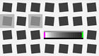 Create and print a test image with the Imatest Test Charts module. A variety of contrast ratios and highlight colors are available. Several Structured vector graphics (SVG) charts are available in Imatest Master. SVG charts with m x n grid patterns (example on right) are well suited for printing large and for automated testing, and have numerous advantages over the ISO 12233 chart.
 - Purchase a chart such as the ISO 12233 (QA-72) or QA-77 (available from Applied Image) or as a less expensive alternative from Danes-Picta in the Czech Republic (the DCR3 chart on their Digital Imaging page). The Applied Image charts are printed with much higher resolution than an inkjet printer can achieve, hence they can be used at much closer distances. Their disadvantage is that they have very high contrasts (>=40:1), which often results in reduced accuracy, and they have a great deal of wasted real estate: usable edges may not be found in regions of greatest interest such as the four corners.
- A printable vector-graphics version of the ISO 12233 chart is available courtesy of Stephen H. Westin of the Cornell University Computer Graphics Department. It should be printed as large as possible (17x22 inches (A2) minimum; 24x36 inches (A1) if possible for 8+ megapixel cameras) so measured sharpness is limited by the camera and lens, not the printer. Because of the limitations of the ISO chart (described above), the Imatest SVG charts are generally preferable.
You
can download printable test charts by right-clicking on the
thumbnails
below. The bitmap chart, which is included in the samples folder of the Imatest
installation, has pixel levels 47 and
255,
has a contrast ratio of (255/47)2.2 = 41 when printed
at gamma = 2.2 (the normal setting). This is close to the minimum
recommended
by the ISO 12233 standard (but higher than optimum; the revised ISO 12233 standard under development will recommend lower contrast). The two SVG charts have contrast ratios of 20 and 2. Instructions for their use can be found in SVG Test Charts. The recommended print size is letter or A4, but these charts print at maximum quality for any size.
| SVG charts — can be viewed, edited, and printed from Inkscape. Right-click on the links to save the file. Download size: 304 KB (SVG); 500 KB (PDF). Printing instructions are here. |
|
Contrast = 20, light, gamma = 2.2, white highlights (SVG) | Contrast = 20 (PDF) High enough contrast to ensure maximum sharpening in most cameras but low enough to avoid clipping most of the time. |
|
Contrast = 2, middle, gamma = 2.2, white highlights (SVG) | Contrast = 2 (PDF) Relatively low contrast: little, if any, sharpening would be expected. The two charts should have the same MTF if no nonlinear processing is applied, for example, with RAW files with dcraw conversion. |
Bitmap chart |
|
|
|
|
Edge_chart_low.png (reduced
contrast;
pixel levels 47, 255) |
|
|
Nonlinear signal processing and chart contrast
Although Imatest SFR is relatively insensitive to chart contrast (MTF is normalized to 100% at low spatial frequencies), measured SFR is often affected by chart contrast due to nonlinear signal processing in cameras, i.e., processing that depends on the contents of neighboring pixels, and hence may vary throughout an image. Nonlinear processing is almost universal in digital cameras (though you can avoid it by using RAW images with dcraw). It improves pictorial quality but complicates measurements. It takes two primary forms.
- Sharpening, applied in the proximity of contrasty features like edges. Boosts response at high spatial frequencies.
- Noise reduction, applied in the absence of contrasty features. Attenuates response at high spatial frequencies, i.e., removes fine, low contrast detail (texture), which is interpreted as noise. Many cameras increase noise reduction at high ISO speeds.
The signal processing algorithms are proprietary; they are a part of a manufacturer's "secret sauce"
for producing pleasing images. Though they vary a great deal, some generalizations can be made.
Most cameras do NOT apply noise reduction and sharpening uniformly throughout an image.
Contrasty edges tend to have better (more extended) MTF than low contrast edges.
For this reason it may be a good idea to photograph both a relatively contrasty edge (though not so high that it causes clipping) as well as a relatively low contrast edge. The SVG charts (above) are excellent choices. Both types of edge can also be produced using Imatest Test Charts. An estimate of chart contrast derived from the average light and dark pixel levels (away from the transition) and gamma is displayed in several places in SFR and Rescharts Slanted-edge SFR. (Estimated chart contrast = (avg. pixel level of light area/avg. pixel level of dark area)^(1/gamma) ).
Nonlinearities are analyzed in depth in the Log F-Contrast module. |
Print the test image (either downloaded or created by Test Charts) from an image editor using a high quality inkjet photo printer on glossy, semigloss, or luster paper. Alternatively, send it to a lab to be printed. Dry Creek Photo has an excellent listing. I recommend printing at least two copies: one for measuring center sharpness and one for edge sharpness. The printed image size should be 8x10 inches (20.3x25.4 cm) or smaller— size is not critical. Be sure the edges look clean and sharp to your eyes; examine them with a good magnifier or loupe. Chart quality is discussed in detail in Chart quality and distance.
The charts should be tilted approximately 5.7 degrees (anywhere between 2 and 7 degrees is OK) when they are photographed. It is tilted 5.7 degrees when the tick marks, located near the edges, are vertically or horizontally aligned with the center. This is illustrated by the red horizontal and vertical lines on the right. Imatest Master can analyze edges of nearly any angle; exact horizontal, vertical, and 45° edges should be avoided for best results. |
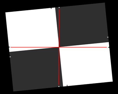
The use of guide marks for tilting the chart
|
The charts are printed straight and physically tilted because the edges print sharper that way. If they were printed at an angle, the printer dot pattern could cause some jaggedness. A 5.71° angle (tan-1(0.1)) is an offset of one part in 10.
Assemble the prints into a target to be photographed.
The following target is described in detail in The Imatest Test Lab. It can be used to measure lens performance near the center, part-way out, and near all four corners. The Log F-Contrast and Star charts to the left and right of center are not necessary for lens testing; they provide information about signal processing. Slanted-edges or other charts (the Kodak Q-14 step chart or the Gretag Macbeth ColorChecker) may be substituted if your primary interest is lens testing.
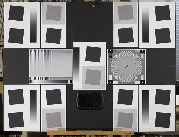
Sharpness target (30x40 inch) for cameras up to 13 megapixels
The printed charts are mounted on a 32x40 inch sheet of 1/2 inch thick black foam board with spray adhesive or double-sided tape. If a ColorChecker is substituted, Velcro is recommended so it can be removed for dark storage. 1/2 inch foam board stays flatter than standard 1/4 or 3/8 inch board. Black board results in less flare light than white board. (Flare light is light that bounces between lens elements and off the inside of the lens barrel, reducing image contrast).
An image of a horizontal or vertical edge on an LCD monitor (desktop or laptop) can also be used as a target. The camera should be tilted with respect to the monitor. The image dark gray and white rather than black and white to minimize clipping. This page contains a description and an image, as well as a description of the Screen Patterns module, which can be used to create an image. The disadvantage of this technique is that you have only one edge to work with; you can't easily create a map of lens performance.
Photograph the target.
Framing
|
Frame the chart so there are usable edges near the center, part-way out, and near the corners. Take care that the chart is properly aligned. A number of useful alignment techniques and tricks are presented in The Imatest Test Lab.
|
|
For a given lens/focal length combination, I recommend testing the lens over a range of f-stops from wide open to fully stopped down. Digital SLR lenses are typically sharpest around f/8. Sharpness is lost to lens aberrations at large apertures and diffraction at small apertures. With Imatest SFR you can find the precise optimum aperture.
Lighting
The chart below summarizes lighting considerations. The goal is even, glare-free illumination. Lighting angles between 30 and 45 degrees are ideal in most cases. At least two lights (one on each side) is recommended; four or six is better. Avoid lighting behind the camera, which can cause glare. Check for glare and lighting uniformity before you expose. A detailed description of the recommended lighting setup, which uses six high quality (CRI > 98) 4700K (near-daylight) 50W SoLux quartz-halogen lamps, can be found in The Imatest Test Lab. SoLux Task Lamps may also be used. The BK Precision 615 Light meter (Lux meter) is an outstanding low-cost instrument (about $100 USD) for measuring the intensity and uniformity of illumination.
Distance
| Distance and field of view |
| The camera must be far enough from the chart so you are measuring the sharpness of your camera and lens, not the chart. But remember, |
It's the field of view, not the chart-to-camera distance, that counts.
|
| A rough rule of thumb: For an inkjet-printed chart the field of view should be at least |
22 inches (60 cm) for a 6-megapixel camera;
35 inches (90 cm) for a 16 megapixel camera. |
| Details below. For a high-quality photographically-printed chart (such as the charts from Applied Imaging) you can get quite a bit closer. |
|
Using a chart printed on Premium Luster paper on the Epson 2200 (a high quality pigment-based inkjet photo printer), the MTF of the 6.3 megapixel Canon EOS-10D showed no change if the image field was at least 22 inches (56 cm) wide-- twice the length of the chart. Performance falls off slowly for smaller widths. Choose a camera-to-target distance that gives at least this image field width. The actual distance depends on the sensor pixel count and the focal length of the lens.
Cameras with more pixels, and hence higher potential resolution,
should
should have a larger image field width. Some guidelines for the minimum
field width are,
| Image field
width (in inches) > 8.8 * sqrt(megapixels)
( > means "greater than.")
Image field
width (in
cm) > 22
* sqrt(megapixels)
-- or --
The distance
to the target
should be at least 40X the focal length of the lens for digital SLRs.
(25X
is the absolute minimum; 40X leaves some margin.) For compact digital
cameras,
which have much smaller sensors, the distance should be at least 100X
the actual
focal length (not the 35mm-equivalent): the field of view is about the same as an SLR with
comparable
pixel count. The recommended distance is described in geeky detail in Chart
quality and distance. |
| The
camera-to-target
distance is not critical as long as it is greater than a reasonable
minimum. |
More on distance can be found in SFR Instructions Part 1.
|
Exposure
|
Proper exposure is important
for accurate Imatest SFR results.
Neither the black nor the white regions of the chart should clip--
have substantial areas that reach pixel levels 0 or 255. The best way
to
ensure proper exposure is to use the histogram in your digital camera.
Blacks (the peaks on the left) should be above the minimum and whites
(the
peaks on the right) should be below the maximum.
|
|
The histogram, taken from the Canon File Viewer Utility, indicates excellent exposure.
| Tips
on photographing the chart |
| Distance
doesn't matter
as long as the target far enough from the camera so sharpness is
limited
by the camera and lens, not
by the target. For a target printed on the Epson 2200 printer, a
distance
that gives at least a 24 inch (horizontal) field of view seems to be
sufficient. |
| The target
should be evenly
lit and free of glare. |
| White
balance should be
approximately neutral. |
| Use a
sturdy tripod and
a cable release. If possible, use the mirror lock. You can use Imatest
SFR to find the difference made by a good tripod or mirror lock. Imatest SFR can
sharpen
your technique, literally ( pun intended ). |
| Be sure to
expose the image
so detail is maintained in both light and dark areas. Neither should be
blocked (clipped). Use your camera's histogram. If more than 0.5% of
the
pixels are at levels 0 or 255, Imatest SFR will assume that clipping
has
taken place and issue a warning message. This has no effect on the
calculations--
it's just a warning that accuracy may be compromised. |
| Be sure
the camera is correctly
focused on the chart. Imatest SFR can test the accuracy of your camera's autofocus. |
| Place
slanted-edge images
near the corners of the field as well as near the center. |
|
Save the image as a RAW file or maximum quality JPEG. If you are
using
a RAW converter, convert to JPEG (maximum quality), TIFF (without LZW
compression,
which isn't supported), or PNG. If you are using film, develop and
scan
it. The file name should be descriptive and should indicate the
parameters
you are testing. Use dashes and underscores ( - and _ ), but try to avoid
spaces, which work with Imatest, but can cause trouble in DOS command
lines
and web pages. An example of a file name is Canon_EOS10D_70-200f4L_100mm_f8.jpg.
If the folder contains meaningless camera-generated file names such as IMG_3734.jpg, IMG_3735.jpg, etc., you can change them to meaningful names that include focal length, aperture, etc., with the View/Rename Files utility, which takes advantage of EXIF data stored in each file.
Run Imatest SFR or Rescharts Slanted-edge SFR
These instructions are excerpted from Using Imatest SFR, Part 2 .
Start Imatest by double-clicking the Imatest icon  on the Desktop, the Windows Start menu, or in the Imatest directory (usually C:\Program files\Imatest in English installations). After several seconds, the Imatest main window opens. Then, either
- Click SFR: New File. The SFR: Current file button is grayed out (inoperative) for the first run because no file has yet been read. It can be used in succeeding runs to save time when analyzing different regions, though multiple ROI (region of interest) runs are more efficient.
- Click Rescharts, then either
- Click Read image file if Slanted-edge SFR is the selected Chart type, or
- Select Slanted-edge SFR from the Chart type: dropdown window.
The Rescharts Slanted-edge SFR module performs the same calculations as SFR, but with more interactive interface, described on the Rescharts page.
Select the image file or batches of files
When you click SFR: New file, the window below appears, requesting the image file name(s). The folder saved from the previous run appears in the Look in: box on the top. You are free to change it. You can open a single file by double-clicking on it.
With Imatest Master you can select multiple files (for combined or batch mode runs) by the usual Windows techniques: control-click to add a file; shift-click to select a block of files. Then click Open. Three image files for the Canon 17-40mm L lens (taken with the EOS-10D) are highlighted. Large files can take several seconds to load. Imatest remembers the last folder used (for each module, individually).
Multiple ROI selection (for batch runs, Imatest Master only).
| Multiple file selection Several files can be selected in Imatest Master using standard Windows techniques (shift-click or control-click). Depending on your response to the multi-image dialog box you can combine (average) several files or run them sequentially (batch mode). |
Combined (averaged) files are useful for measuring the effects of image stabilization. The combined file can be saved. Its name will be the same as the first selected file with _comb_n appended, where n is the number of files combined. |
Batch mode allows several files to be analyzed in sequence. There are three requirements. The files should (1) be in the same folder, (2) have the same pixel size, and (3) be framed identically. |
The input dialog box for the first run is the same as for standard non-batch runs. Additional runs use the same settings. Since no user input is required they can run extremely fast. |
If the order of the files in a batch runs is different from the selection order, click Settings, Options and Settings... (in the Imatest main window) and change the setting in Batch run order. The sequence may be affected by Windows Explorer settings. |
One caution: Imatest can slow dramatically on most computers when more than about twenty figures are open. For this reason we recommend checking the Close figures after save checkbox, and saving the results. This allows a large number of image files to be run in batch mode without danger of bogging down the computer. |
|
Select the ROI (Region of Interest)
If the image has the same pixel dimensions as the last image in the previous run, a dialog box asks you if you want to repeat the same ROIs (regions of interest) as the previous image. You can retrieve saved ROIs from past runs by clicking on Retrieve settings in the Imatest main window prior to selecting SFR.
If you answer No or if the image has a different size, the coarse selection dialog box shown on the right is displayed with the instructions, Select ROI by clicking and dragging, or clicking outside image. Click on one corner of the intended region, drag the mouse to the other corner, then release the mouse button. Click outside the image to select the entire image.
After you make your selection, the ROI fine adjustment dialog box (below) appears. You can move the entire ROI or any of the edges in increments of one pixel. You can also enter the ROI boundary locations in the boxes below the image. If you do this, be sure to press return (or move the cursor) to register the change. You can zoom out to view the entire image, then zoom back in. |
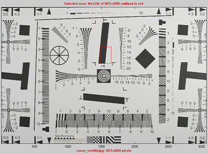
ROI selection using ISO 12233 chart
(popular, but has much wasted area)
|
When you are satisfied with the ROI selection, proceed by selecting one of five choices at the bottom of the box. The ROI fine adjustment is particularly valuable for working with tiny regions and excluding interfering detail.
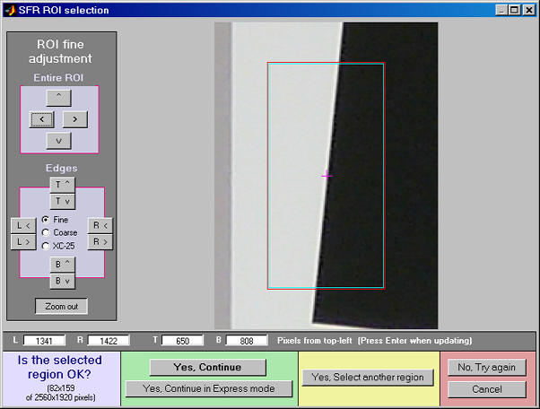
ROI fine adjustment
| Yes, Continue |
The selected ROI is correct; no more ROIs are to be selected. Continue with SFR calculations in normal mode: You will be asked for additional input data, etc. |
| Yes, Continue in Express mode |
The selected ROI is correct; no more ROIs are to be selected. Continue with SFR calculations in Express mode: You will not be asked for additional input data or for Save options. Saved or default settings will be used. |
| Yes, select another region |
The selected ROI is correct. Select another ROI. For multiple ROIs additional Figures will display performance as a function of distance from the image center. |
| No, try again |
The selected ROI is not correct. Try again. |
| Cancel |
Cancel the SFR run. Return to the Imatest main window. |
|
If the selected area is too small, too large, or inappropriate, you'll be asked to repeat the selection. The ROI is normally checked for validity, but there are some cases (e.g., endoscopes) where valid images may fail the usual tests ROI filtering can be relaxed considerably by opening the Options and Settings... button in the Imatest main window (Pro only) and clicking Light filtering in the first group of controls. This can can lead to errors when regions are selected carelessly. Normal filtering is the default.
After the run is complete, you can save ROIs for future runs in a named file by clicking on Save settings in the Imatest main window. These settings can be retrieved later by clicking on Retrieve settings.
Cropping recommendations
For best accuracy the length should be between about 80 and 500 pixels. In most cases little is gained for lengths over 300 pixels.
The width (height in the image on the right) should be at least 50 pixels. The light and dark zones should be at least 10 pixels wide, with 20 preferred. Little is gained for minimum dark/light zone widths over 40 pixels or total width over 100 pixels.
|
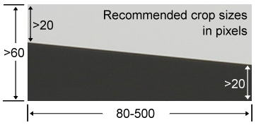 |
My typical crops are between around 120x80 and 300x140 pixels.
The absolute minimum and maximum crop dimensions are 10 and 1200 pixels (800 for strong ROI filtering). For very small crops (width or length less than about 25 pixels) a warning message may appear in place of the light/dark level display: Zero counts in n bins. Accuracy may be reduced. This indicates that some interpolation was required to obtain the final result, and that you should be aware that results may not be as accurate or repeatable as they would be for larger ROIs. Small crops or noisy images may require weaker error filtering than normal crops/images. Press Options & Settings... in the Imatest main window and set SFR ROI filtering to Light filtering.
SFR input dialog box
After you select the Region(s) of Interest (ROI(s)) the Imatest SFR input data window appears, unless Express mode has been selected. All input fields are optional. Most of the time you can simply click OK (the box on the lower right) to continue. Selections are saved and can be used for future express runs. The input data window is described fully in SFR instructions, Part 2. It is divided into sections: Title and Help on top, then Plot, Options, Settings, Optional parameters, and finally, OK or Cancel. Here are a few highlights.
SFR input dialog box (full version)
Plot This area controls which figures to plot. Figures are listed on the left. Plot settings are saved between runs. The boxes adjacent to "Cycles per" control the x-axis display for MTF plots. You can choose between Cycles per pixel (the default), Cycles per inch, or Cycles per mm. If you choose Cycles per inch or mm, you must enter a number for the pixel size— either in pixels per inch, pixels per mm, or microns per pixel. If pixel size is omitted, the x-axis will be displayed in Cycles per pixel. For the second plot you can choose between LW/PH and LP/PH (Line Pairs per Picture Height).
Display options affects the appearance of plots.
- Secondary readout (defaults to MTF30, the spatial frequency for 30% contrast; MTF50 is the primary readout.) Can be set for MTFnn or MTFnnP at any contrast level or to MTF at a specified spatial frequency in cycles/pixel, line pairs/inch or line pairs/mm. For example, you might select MTF at the half-Nyquist frequency, 0.25 cycles/pixel. Details.
- MTF plot freq selects the maximum display frequency for MTF plots. The default is 2x Nyquist (1 cycle/pixel). This works well for high quality digital cameras, not for imaging systems where the edge is spread over several pixels. In such cases, a lower maximum frequency produces a more readable plot. 1x Nyquist (0.5 cycle/pixel), 0.5x Nyquist (0.25 cycle/pixel), and 0.2x Nyquist (0.1 cycle/pixel) are available.
- Edge plot selects the contents of the upper (edge) plot. Three displays are available. 1. Edge profile (linear) is the edge profile with gamma-encoding removed (the default). 2. Line spread function (LSF) is the derivative of the linear edge profile. 3. Edge pixel profile is proportional to the edge profile in pixels, which includes the effects of gamma encoding. The edge can be cropped (default) or the entire edge can be displayed.
- Chart contrast For a medium or low contrast charts (contrast <= 40; not recommended with the old ISO 12233 chart), you can enter the chart contrast (or Off). If the ROI is large enough, the actual (measured) gamma will be calculated and displayed along with the contrast factor (the chart contrast multiplier = measured gamma/nominal gamma, where nominal gamma is entered in the Settings area, described below). If the Use for MTF box just to the right is checked, this value will be used in the MTF calculation, which may result in a modest improvement in accuracy.
- Reset restores the settings in Options and Settings to their default values.
Settings (affects the calculations)
- Standardized sharpening is a software "filter" applied to a camera's MTF response that facilitates comparisons between cameras by compensating for different degrees of sharpening. Standardized sharpening display, which appears as red dashed curves ( − − − − ) in the edge and MTF plots, is selected with the checkbox. Radius controls the sharpening radius. The default value of 2 (pixels) is works well for many compact digital cameras; it is often smaller for Digital SLRs, and can be different for different RAW converters. For very broad transitions, the radius is automatically increased unless Fixed sharpening radius in the Settings menu of the Imatest main window has been checked.
For more detail, see What is standardized sharpening, and why is it needed for comparing cameras?
| Standardized sharpening should be unchecked for most lens tests. Standardized sharpening tends to "flatten" lens comparisons, though it can give a useful indication of what to expect after sharpening. |
- Gamma is the exponent of the curve that relates scene luminance to pixel level. It is explained briefly in the glossary and in detail here. It defaults to 0.5, which is typical of digital cameras, but it is affected by camera (or RAW converter) contrast settings. Gamma is reliably 0.5 when RAW files converted with dcraw are entered into Imatest. Gamma is used to convert pixel levels back to the linear scale required to calculate MTF. A 10% error in gamma results in a 2.5% error in MTF50. If you have doubts about the value of gamma, I recommend running Colorcheck or Stepchart. A nominal value of gamma should be entered, even if the value of gamma derived from the chart (described above) is used to calculate MTF.
- Channel is normally left at it's default value of Y for the luminance channel,
where Y = 0.3*R + 0.59*G + 0.11*B.
In rare instances the R, G, and B color channels might be of interest.
- (Standardized sharpening unchecked ): Standardized sharpening results are replaced with RMS Edge roughness in pixels and MTF50P: the frequency where MTF drops to half its peak value— a useful indicator of the performance of heavily-sharpened cameras without post-processing. (MTF50P = MTF50 for cameras with weak to moderate sharpening.) The plots for the separate RGB channels are emphasized, but the MTF summary .CSV output is unchanged.
- Picture Width and Height defaults
to the width and height of the input image in pixels, assuming landscape format,
where height < width. If the input image
has been cropped, or if it doesn't represent the entire camera image, Picture
Height (and Width) should be entered manually.
When entries are complete, click OK. A Calculating... box appears to let you know that calculations are proceeding. Results appear in individual windows called figures (Matlab's standard method of displaying plots). Figures can be examined, resized, maximized, and closed at will. Their contents are described in MTF (Sharpness) plot, Chromatic Aberration, Noise, and Shannon Capacity plot, and Multiple ROI (Region of Interest) plot.
Two precautions when working with figures
Too many open Figures
Figures can proliferate if you do a number of runs, especially SFR runs with multiple regions, and system performance suffers if too many Figures are open. You will need to manage them. Figures can be closed individually by clicking X on the upper right of the Figure or by any of the usual Windows techniques. You can close them all by clicking Close figures in the Imatest main window. |
Clicking on Figures during calculations
can confuse Matlab. Plots can appear on the wrong figure (usually distorted) or disappear altogether. Wait until all calculations are complete— until the Save or Imatest main window appears— before clicking on any Figures. |
Save the results
At the completion of the SFR calculations the Save SFR results? dialog box appears (unless Express mode has been selected). It allows you to choose which results to save and where to save them. Selections are saved for future runs. The default is subdirectory Results of the data file directory. You can change to another existing directory, but new results directories must first be created outside of Imatest using a utility such as Windows Explorer. (This is a limitation of this version of Matlab.)
Figures, CSV, and XML data are saved in files whose names consist of a root file name with a suffix and extension. The root file name defaults to the image file name, but can be changed using the Results root file name box. Be sure to press enter.
When multiple ROIs are selected, the Save results? dialog box appears only after the first set of calculations. The remaining calculations use the same Save settings.
The first four checkboxes are for the figures. 5-7 are for Excel .CSV results. 8 is for XML output. You can examine the output figures before you check or uncheck the boxes. Checking Close figures after save closes figures after they are saved. This can be useful for large batch runs (Imatest Master only), where too many open figures will degrade the performance of most computers. Details of the output files can be found here. |
SFR Save dialog box. |
The following table lists figures and Excel-readable CSV files produced by Imatest SFR.
Output files
for filename.jpg (Y-channel)
(default location:
subfolder Results)
| Figures
(.PNG image files) |
| filename_YA17_cpp.png |
Plot with x-axis in cycles/pixel (c/p), Y-channel,17% of the way to
the corner above the center of the uncropped image. |
| filename_YA17_lwph.png |
Plot with x-axis in Line Widths per Picture Height (LW/PH). |
| filename_YA17_ca.png |
Plot of Chromatic Aberration, with noise statistics and Shannon information
capacity. |
| Excel
.CSV (ASCII text files that can be opened in Excel) |
| CSV output files are explained in detail below. Click link for detail on individual file. |
| SFR_cypx.csv |
(Database file for appending results: name does not change). Displays
10-90% rise in pixels and MTF in cycles/pixel (C/P). |
| SFR_LWPH.csv |
(Database file for appending results: name does not change). Displays
10-90% rise in number/Picture Height (/PH) and MTF in Line Widths per Picture
Height (LW/PH). |
| filename_YA17_MTF.csv |
Excel .CSV file of MTF results for this run. All channels (R, G, B, and Y (luminance) ) are displayed.The first row has the
headers: cy/pxl, LW/PH, MTF(nchan), MTF(corr), MTF(R), MTF(G), MTF(B), MTF(Y), where nchan is the selected channel. The remaining lines contain the
data. Can easily be plotted or combined with data from other files. |
| filename_Y_multi.csv |
Excel .CSV file of summary results for a multiple ROI run. |
| filename_Y_sfrbatch.csv |
Excel .CSF file combining the results of batch runs (several files) with multiple ROIs. Particularly useful for generating easily-readable Excel plots. |
Repeated runs
If SFR was previously run with an image of the same pixel dimensions and you click on either of the Run
SFR buttons, an image that displays the selected ROIs
appears on the left of the screen and you'll be asked, "Do
you want the same ROIs as the previous image?" A portion
of the previous image and the ROI repeat box for Imatest Studio are shown in the image on the right. Two additional options are available for Imatest Master.
|
ROI repeat dialog box: Imatest Studio
(Pro below) |
| Yes |
Use the previous crop. Open SFR input dialog box. |
| Yes, Express mode |
Use previous crop and run in Express mode.
Do not open the
input dialog box;
use saved data instead. Save dialog boxes are also omitted.
Some warnings are suppress. Speeds up repeated runs, e.g., testing several apertures. |
| Yes, Adjust ROI |
Open a fine adjustment dialog box (shown below), starting with the previous selection.
Useful for a sequence of runs with similar, but not identical, framing.
Imatest Studio: Only available when a single ROI is selected.
Imatest Master : For multiple ROIs, a window that allows ROIs to be shifted and changed in magnification is opened. |
| No |
Crop the image using the Select the ROI... dialog box described above. |
| Cancel |
Cancel the run. Return to the main Imatest window. |
Automatically refine ROIs
Yes |
Imatest Master only
Refine previous crop (see description below) and run in Express mode. |
Automatically refine ROIs
Yes, Express mode |
Imatest Master only
Refine previous crop (see description below). Open SFR input dialog box. |
Multiple ROI fine adjustment (Imatest Master only)
When different cameras or lenses (or different focal lengths in zoom lenses) are tested using the same target, it is not generally possible to maintain exact alignment from image to image. Starting with Imatest Master 2.6 there are two options for refining (shifting) ROI selections during repeated runs: the Multiple ROI fine adjustment dialog box and Automatic ROI refinement, described below.
The Multiple ROI fine adjustment dialog box, shown greatly reduced on the right, is opened if the previous run used multiple ROIs and Yes, Adjust ROI(s) is selected in the ROI Repeat dialog box. It allows all ROIs or individual ROIs to be shifted (up, down, left, or right), enlarged, and shrunk, and the magnification to be changed. This operation may be followed by Automatic ROI refinement if either of the buttons on the right is pressed.
|
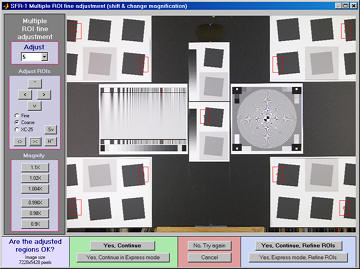
Multiple ROI fine adjustment dialog box:
Imatest Master
|
Automatic ROI refinement (Imatest Master only)
This option is very useful for sequences of runs where chart alignment varies slightly; it can be especially valuable for Imatest API in manufacturing environments.
The Imatest Master ROI repeat dialog box offers two options in the light blue box on the right (Yes and Yes, Express mode) that include automatic ROI refinement. Results of the refinement are shown in the crop of the Multi-ROI 2D summary plot on the right. The original (incorrect) ROIs are shown as cyan rectangles; the automatically refined (shifted) ROIs are shown as bold red rectangles filled with the full contrast image.
Automatic ROI refinement works best with charts dedicated to SFR measurement such as the SFR SVG test charts. It may not work as well with the ISO 12233 charts because of the narrowness of the SFR strips and the presence of interfering patterns.
The length of the ROIs should be no larger than 85% of the length of the edge to be measured. Automatic refinement will succeed if no more than 30% of the ROI length is off the edge. The modified ROI is not saved in imatest.ini.
|
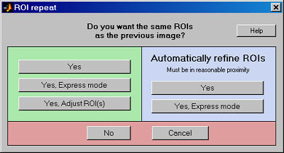
ROI repeat dialog box: Imatest Master
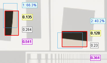
Results of automatic ROI Refinement:
Original (cyan) and refined (bold red)
|
Interpret the results
Multiple regions If you selected multiple regions of interest and checked one of the 2D image plots in the Multi-ROI plots section of the input dialog box, as shown above, the following summary display appears.
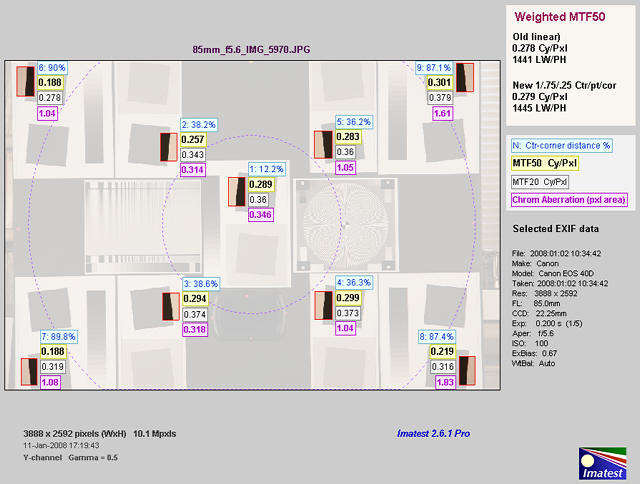
Multi-ROI 2D summary plot, showing Center-corner distances,
MTF50, MTF20, and Chromatic Aberration (in pixels) superimposed on image.
This display, introduced with Imatest 2.5.8, can be particularly useful because lenses are not always centered properly. (If they were, performance would be a simple function of the distance from image center.) You can quickly scan the summary results, then look at the detailed results for the individual region. The legend explaining the four results boxes next to each ROI is on the right. The boxes contain (1) The ROI number (N) and the center-to-corner distance expressed in %, (2) MTF50 in either cycles/pixels or LW/PH, in boldface for emphasis, (3) MTF20, and (4) Chromatic Aberration in pixels of area.
If you saved the CSV summary output files for sequences of multiple ROI runs (for example, for a sequence of apertures: f/4, f/5.6, f/8, f/11, ...) or if you did a batch run using multiple ROIs, you can combine data from several runs and produce concise summary plots in Excel. The technique is described here. Here is an example.
Summary plot for 6 multi-ROI runs (f/5.6-f/32) for the Canon 17-85mm IS lens, EOS-40D (JPEG)
The Excel file was created by combining single-column summary results
from the CSV summary output files for the 6 runs.
Edge and MTF display.
Single region detail The most detailed Imatest SFR figure, shown on the right, contains the average edge profile on top and MTF (spatial frequency response) on the bottom. (Input-related data on the right of the figure is omitted here.)
Although the edge response in the upper figure is relevant to sharpness, the MTF curve in the lower figure is the preferred measurement because
- MTF, and especially MTF50 or MTF50P, the spatial frequencies where contrast drops to half its low frequency or peak levels, correlate well with perceived image sharpness, and
- System MTF response is the product of the MTF of individual components. No such simple formula is available for edge responses.
SQF— Subjective Quality Factor is the best measurement of perceived print sharpness because it includes the contrast sensitivity of the human visual system, print size, and estimated viewing distance, in addition to MTF. Its importance will grow as it becomes more familiar. SQF is strongly affected by sharpening.
Other numbers are available for evaluating lenses. The Secondary readout feature allows you to select (spatial frequency for) MTF at any level or MTF at a spatial frequency specified in Cycles/pixel, lp/mm, or lp/in. For example, you could use MTF30 (which results in a higher spatial frequency), or MTF at a fixed spatial frequency (as is done in manufacturer's data sheets, which typically give contrast (MTF) at 10, 20, and 40 (or 10 and 30 line pairs/mm). If you do this you may want to scale the x-axis to cycles (i.e., line pairs) per mm instead of the default cycles/pixel.
Remember, in evaluating lenses, use the results without standardized sharpening (the black curves and text). It's best to uncheck the Standardized sharpening box. Results with standardized sharpening do, however, have some interest: they indicate what can be achieved after sharpening. But they tend to "flatten" differences between lenses.
Clipping can reduce the accuracy of calculations, though the amount of clipping is a poor indicator of the reduction in accuracy. Click here to learn more.
To learn more about sharpness measurements, see Sharpness: What is it and how is it measured?, SFR Tour, and SFR Results: MTF (Sharpness) plot.
Chromatic Aberration is an important aspect of lens performance. CA is best measured on tangential edges near the borders of the image. The best measure of CA is the percentage of the distance from the image center. Interpretation: under 0.04; insignificant. 0.04-0.08: minor; 0.08-0.15: moderate; over 0.15: serious.
For more information, see Chromatic Aberration and SFR Results: Chromatic Aberration ... plot. |
Chromatic Aberration display. |
Checklist
License holders are encouraged to publish test results in printed publications, websites, and discussion forums, provided they include links to www. imatest.com. The use of the Imatest Logo is encouraged. However you may not use Imatest for advertising or product promotion without explicit permission from Imatest LLC. Contact us if you have questions.
Imatest LLC assumes no legal liability for the contents of published reviews. If you plan to publish test results, you should take care to use good technique. This list summarizes the key points presented above. It's well worth reviewing.
| Sturdy camera support |
Use a sturdy tripod, cable release, and, if possible, mirror-lock. |
| Target mounting |
If you are working outdoors, be sure the target doesn't shake in the wind. |
| Target distance |
Be sure you're far enough fro the target so the printed edge quality doesn't affect the measurements. Target distance considerations are given here. |
| Focus |
Be sure the camera is focused accurately on the target. Note whether you used manual or automatic focus. |
| Target alignment |
Make sure the corners, as well as the center, are in focus. |
| Raw conversion and settings |
The choice of RAW converter (in or out of the camera) and settings, particularly Sharpening, can make a huge difference. Contrast and White balance are also important. Settings that affect contrast and transfer curve can also have a strong effect. If possible a "Linear" setting (meaning a straight gamma curve with no additional tonal response adjustments) should be used. |
Gamma
|
SFR sharpness results are moderately sensitive to the Gamma setting: A 10% gamma error changes MTF50 by 2.5%. For best results gamma should be measured by running Colorcheck or Stepchart. Ideally a Q-14 target (similar to the Q-13, but larger) should be mounted close to the slanted edge images. |
| Cleanliness and filters |
Lens surfaces should be clean. You should note whether you have a protective (UV or Skylight) filter. It can make a difference— more likely reduced contrast than reduced sharpness. With Imatest you can find out. |
| File formats |
Use RAW or the highest JPEG quality. Never use less than the maximum resolution or JPEG quality unless you are specifically testing the effects of these settings. |
| Lens settings |
Lens performance is a strong function of the aperture (f-stop) and focal length (for zooms). Be sure to record these settings (easy because they're saved with the EXIF data) and include them in your writeup. The optimum (sharpest) aperture is of particular interest. Lens performance is also somewhat affected by the distance to the target. |
| White balance |
Should be close as possible to neutral, particularly in Colorcheck. |
This may seem like a lot of fuss, but the technique you develop in testing cameras and lenses will spill over to your daily photography. Alfred Stieglitz tested film and developers extensively when he discovered photography as a student in Berlin. Ansel Adams performed extensive tests in the development of his zone system. Although nobody would claim that testing is responsible for their unique vision, it certainly contributed to the skill that transformed their vision into prints of transcendent beauty.
The Imatest Test Lab
How to build a testing lab
The Imatest Laboratory was set up for several purposes.
- To demonstrate how to construct a cost-effective image quality testing lab.
- To validate new Imatest modules and image quality testing concepts.
- To perform tests for clients who need low volumes of testing or want to verify their own testing methods.
- To photograph artwork. The optimum setup for measuring image quality is, not coincidentally, optimum for photographing fine art.
The lab was designed to meet the following goals.
- Low cost, easily obtainable, high quality components.
- Portable: easy to move if needed.
Hardware
Substitutions can be made for most of the parts listed below. Creativity is encouraged in assembling a lab.
Lighting
To obtain high quality illumination covering up to 40x60 inch (100x150 cm) foam board with reasonably good uniformity and smaller areas with high uniformity, we selected a track lighting system that takes the outstanding SoLux 4700K (near daylight) 12V MR16 halogen lamps, which use long-lasting built-in dichroic filters.
Fixture. The Hampton Bay K15 expandable halogen track lighting kit (724-491), available from Home Depot, along with the A18 end connector with cord and switch (678 546) is inexpensive and excellent. It's not on their website. Similar products should work equally well, for example, the Pro Track 150 Watt Low Voltage Track Kit
(65227) from Lamps Plus. |
|
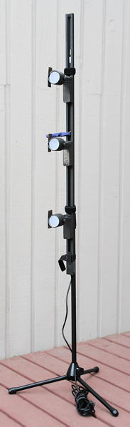
Lights & stand |
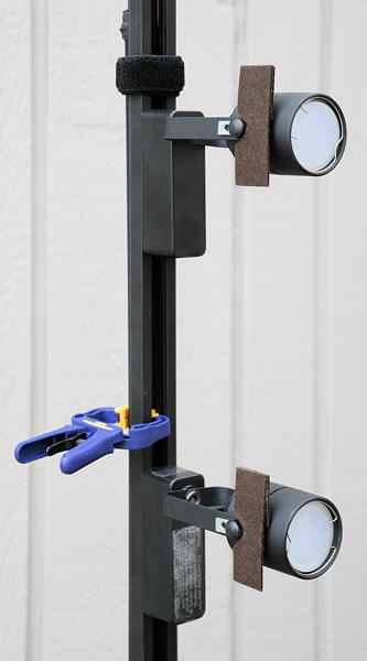
Lamp detail |
Lamps. We use 6 SoLux 50W 4700K/36 degree MR16 bulbs, along with 6 Plano Convex diffusers, which are necessary for even light. The diffusers are mounted in front of the lamps (rightmost image), in place of the clear glass supplied with the track lighting kit. "T" braces with self-adhesive felt pads were added to the sides of the lamp fixtures to block stray light from reaching the lens (rightmost image).
SoLux halogen bulbs are inexpensive and produce extremely high quality near-daylight 4700K illumination, with a CRI (Color Rendering Index) of 98 out of 100. They were featured in a recent article in Inkjetart.com. SoLux also sells track lighting components.
Stand. The Radio Shack 33-335 folding microphone stand is simple, lightweight, sturdy, and cheap.
Assembly. The track is attached to the stand with an 8-32 bolt. Here is the procedure.
Drill holes large enough for an 8-32 bolt about 1.25 inches (3.5 cm) below the top of the upper shaft of the microphone stand and about 10 inches (25cm) below the top of the track (the end without the cord). The head of a 1.25 or 1.5 inch 8-32 bolt is placed inside the track, then attached with two nuts on the back of the track to provide a little spacing with the stand. A wing nut (optional) is used to secure the bolt to the stand. [Parts sequence: 8-32 bolt (head), track, 2 8-32 nuts, upper shaft of microphone stand, 8-32 wing nut.] (CAUTION: do not do this unless you know how to work with electrical wiring safely. DO NOT do this when the track is plugged in! )
The remainder of the track is attached to the stand by a combination of materials that allow the stand to be raised and lowered.
- Cambuckles and nylon webbing. Nice because they put tension on the webbing when they are closed. 1 inch and 2 inch Available from REI.
- Strapall heavy-duty Quick Tape, available from REI and many other sources. This is a strong double-sided Velcro tape.
- Sticky-back Velcro tape. Can attach to both the mic stand and the back of the track, but contact area is limited.
The lights are mounted near the top, middle, and bottom of the 40 inch high targets.
If you have a large budget and need high intensity illumination, check out the Imaging Resource laboratory-grade lighting system, which uses HMI lamps.
Easel
The Mabef M-10 easel was chosen because it was sturdy, could be adjusted vertically (checked with a small level), had just the right features, and was on display at a local art supply store. A self-adhesive felt pad on the bottom of the upper clamp helps secure targets. |
 |
Light measurement
The BK Precision 615 Light meter (Lux meter) is an outstanding low-cost instrument (about $100 USD) for measuring incident light (illuminance). It has a flat diffuser and photopic response (similar to the human eye in bright light). It is particularly useful for measuring evenness of illumination. We purchased ours from Action Electronics, which offers several alternative choices. The BK was chosen over similar Easyview meters because it has a flat (rather than hemispheric) diffuser that better represents the geometry of the flat targets. Readings can be somewhat slow, with settling times around 3-5 seconds.
Miscellaneous
Several additional items can come in handy: a small level, a flashlight (LED models are cool), rulers, a few clamps, etc. A bubble level mounted on a camera's accessory shoe can be particularly helpful. A few Irwin Quick-Grip Handi-Clamps are useful for attaching the targets to the easel. |
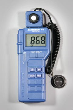 |
Tripod and accessories
The tripod should be sturdy, easy to adjust, and easy to move. Any good tripod with a pan/tilt head should work. Ball heads are not recommended for the lab. A head that takes quick-release plates is strongly recommended. Any tripod can be adapted for quick release with the Bogen/Manfrotto RC2 adaptor, which is supplied with one 3157N plate. We illustrate a few Manfrotto components, which offer good value for the price. These represent typical choices; many more are available to meet special needs.
Manfrotto 475 or 475B tripod legs with geared center column - supports 26.5 lbs. Height 16.6 – 74 in. A geared center column is not strictly necessary (we don't have one on our old Bogen/Manfrotto 3021BN), but can be convenient in a tripod dedicated to a test lab. The built-in spirit level is valuable for leveling the tripod: If the base (where the head is mounted) is level, fine adjustments are much easier to make because head movements (swivel, etc.) don't interact.
Manfrotto 804RC2 3-way pan-tilt head with quick release - supports 8.8 lbs. A very nice head, very reasonably priced. Uses the versatile RC2 quick release system. Get several 3157N mounting plates if you purchase this head. |
|
Manfrotto 3275 / 410 compact geared head with quick release - supports 11.1 lbs. A more elegant but more expensive head: especially nice for making precise adjustments. Uses the less common 3271 quick release mounting plate.
Manfrotto 3137 variable leg spread portable dolly. Very useful for keeping legs in place while moving the tripod.
804RC2 pan/tilt head |
3275/410 geared head |
Manfrotto 3137 dolly |
 Manfrotto 3416 leveling head. Optional. The level built into the 475B (and several other) legs may suffice for most users. Mounts between the tripod legs and the head. Ensures that the base of the head is level so that the various movements (swivel, etc.) don't interact. This greatly facilitates fine adjustments.
Clamps
Although a regular quick-release tripod mount is fine for most cameras, a good sturdy clamping system is needed for testing cameraphones and webcams. We put two of them together after rummaging through the aisles of Home Depot. They consist of Irwin Quick-Grip Mini or Micro bar clamps mounted on Manfrotto quick release plates. The images below give a good idea of how they're constructed. A hole had to be drilled in the larger clamp (above) and enlarged in the lower clamp (below) to accommodate the 1/4 inch bolt.
Clamp parts (top to bottom)
|
Larger (Mini) clamp (above)
1.5" long 1/4" bolt
1/4" coupling nut
Irwin Quick Grip Mini bar clamp
1/4" coupling nut
"T"-brace
Quick release plate
|
Smaller (Micro) clamp (below)
3/4" long 1/4" bolt
1/4" washer
Irwin Quick Grip Micro bar clamp
large 1/4" washer
1/4" coupling nut
"T"-brace
Quick release plate |
The larger clamp (the Mini) is sturdier, and has proven to be more useful.
Putting it together
The image below summarizes how the lights should be positioned. The goal is even, glare-free illumination. The lamps represent the stacks of three SoLux track lamps, described above. This may involve a tradeoff, especially with wide-angle lenses. Lighting angles between 35 and 45 degrees work well for normal and long lenses. Avoid lighting behind the camera, which can cause glare. Ambient light should be kept subdued. Check carefully for glare and lighting uniformity before you expose, especially with wide angle lenses, where glare can be difficult to avoid: you may have to move the lights further than normal from the target— or allow glare in portions of the target, taking care that it doesn't affect critical areas.
Use the meter to check for the evenness of lighting. ±20% over the entire target is sufficient for SFR and Distortion measurements, where small portions of the target are analyzed and exposure is not critical. ±5% or better should be the goal for tonal and color measurements (Stepchart, Colorcheck, and Multicharts). This should be easy to achieve because illumination only needs to be even on the relatively small charts themselves, not on the entire target. The widest (the Kodak Q-14) is 14 inches (35 cm) wide; most are under 11 inches (28 cm). Lighting uniformity is strongly affected by the distance and orientation of the lamps. Our lamps are roughly 50 inches (125 cm) from the center of the target.
Targets
Charts are mounted on 40x60 inch (100x150 cm) or 30x40 inch (75x100 cm) 1/2 inch (1.25 cm) thick foam board, which is lightweight, rigid (unlikely to warp), and easy to find at art supply shops. The images below show entire targets. Framing would normally be tighter for test images (much tighter for the Q-14, ColorChecker, and OECF targets). In some cases, the charts are mounted on neutral, middle gray (~18% reflectance) mat board, which is attached to foam board, to ensure correct exposure in cameraphones and webcams with autoexposure.
Charts are mounted using permanent double-sided tape or spray adhesive, available from hardware and art supply stores. We have used 3M 45 and 3M Photo Mount sprays, both of which are "Photo safe." 3M Super 77™ is not labeled "Photo safe," (and can't be sold in California), but it should be OK for attaching gray mat board to foam board.
Sharpness targets
The SFRplus chart, introduced with Imatest 3.2, features automated detection of up to 23 regions for sharpness measurements. It offers numerous advantages over the well-known ISO 12233 chart, particularly more accurate measurements due to reduced contrast, sufficient regions to produce a good lens response map, and compatibility with automatic region detection. SFRplus also measures distortion, tonal response, gamma (contrast), and color accuracy for the color chart (shown below). It is especially useful for automated testing. SFRplus charts are available for purchase.
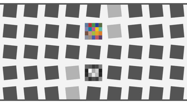
SFRplus color chart (ideal values shown)
Two additional sharpness targets are also used in the Imatest lab, though less frequently than the SFRplus chart. Both consist of several charts printed on Epson Enhanced Matte (Ultra Premium Presentation - Matte) paper, which resolves detail as well as semigloss and glossy inkjet papers, but is much less susceptible to glare. These charts support SFR as well as several Rescharts modules (SFR, Log F-Contrast, Log Frequency, and Star Chart).
Sharpness target (30x40 inch) for cameras up to about 16 megapixels
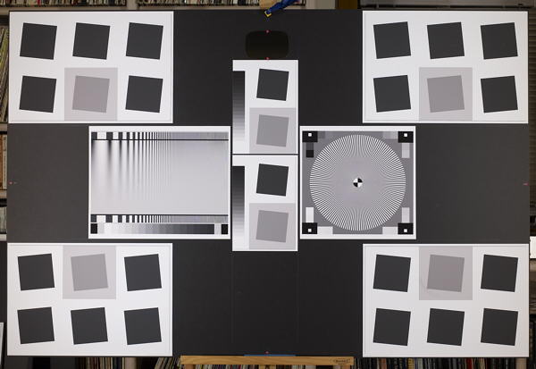
Sharpness target (40x60 inch), for cameras over about 16 megapixels
(recommended for cameras over 8 megapixels)
Target size
|
40x60 inches (100x150 cm) |
30x40 inches (75x100 cm) |
Chart
location | For images over 13 megapixels;
Recommended for images over 8 megapixels |
For images up to 13 megapixels |
| Center |
1x2 SVG SFR chart, 20:1 and 2:1 contrast, trimmed. |
2 – 1x2 SVG SFR charts, 20:1 and 2:1 contrast, trimmed. |
| Right of center |
Standard 144-cycle sinusoidal Siemens Star chart, printed 30 cm (11.81 inches) high on 13x19 inch paper, trimmed on left and right. |
Standard 144-cycle sinusoidal Siemens Star chart, printed 20 cm (7.87 inches) high on US letter-size paper |
| Left of center |
Log F-Contrast chart, printed 30 cm (11.81 inches) high on 13x19 inch paper |
Log F-Contrast chart, printed 20 cm (7.87 inches) high on US letter-size paper |
| Corners |
SVG Squares 2x3 (Same orientation). Two of the charts must be printed as mirror images to obtain approximately radial and tangential edges: in Inkscape, select the chart, then click on Object, Flip Horizontal before printing. |
1x2 SVG SFR chart, 20:1 contrast. See note on left about printing mirror images. |
| Inside (L,R) of corners |
N/A |
1x2 SVG SFR chart, 20:1 and 2:1 contrast, trimmed to remove step chart. See note on left about printing mirror images. |
| Mirror |
Mount a mirror, centered horizontally on the target, above or below the center charts. Automotive mirror replacement glass (easy to find in automotive supply shops) or hobby/cosmetic mirrors should do. Mark the center of the chart (with a sticker, bright pen, etc.). Use the "rope trick" described below to center the camera horizontally. |
Notes on the charts:
- MTF measurements for the two charts were compared using a 39-megapixel medium format camera with an excellent lens. MTF was approximately 10% higher when measured on the 40x60 inch target. That is the basis of the above recommendation that the larger chart be used for cameras with over 13 megapixels.
- The mirrors are difficult to see in the above images because they are reflecting a darkened room on a dark background. The mirror above the center of the 40x60 inch target is illustrated on the right.
- The 20:1 slanted edges are used as the standard edges for SFR sharpness measurements. They are arranged so sharpness can be measured near the image center, half-way between the center and the four corners, and near the corners. This is important because lens response may be asymmetrical in lenses that are decentered due to sloppy manufacturing. This contrast is lower than the minimum specified by the ISO standard (40:1), which is now understood to result in large errors if gamma is poorly estimated or if the tonal response is nonlinear (clips or deviates from a straight gamma curve). Much lower contrast will be recommended in the revised ISO standard.
- The 2:1 slanted edges measure MTF in regions where contrasty edges are absent. In such regions there may be less software sharpening; software noise reduction (lowpass filtering; the opposite of sharpening) may be employed. Signal processing that differs in different parts of the image is called nonlinear.
|
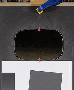
Mirror, showing red dot • stickers
marking the horizontal target center |
Aligning the camera with the target
To obtain the most accurate and consistent results from Imatest's spatial measurements (sharpness, chromatic aberration, and distortion), the camera and target must be aligned presicely. This means that
- The axis of the lens should be normal (perpendicular) to the surface of the target,
- The edges of the image should be parallel with the edges of the charts in the target,
- In most cases, the center of the image corresponds to the center of the target.
Accurate alignment is easy to obtain with an optical bench, but optical benches large enough for Imatest testing are extremely expensive. For this reason users need to develop a collection of tricks to facilitate alignment for different cameras, lenses, or focal lengths.
Leveling (horizontal, vertical (front/back))
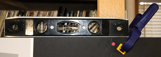
Level the target horizontally (illustrated above) and vertically (front/back) (illustrated on the right). Then mount a spirit (bubble) level on the camera (shown below) and level the camera horizontally and vertically. This gets the leveling very close to the final setting. The "Adorama Double Bubble Level" (sounds like chewing gum) costs about $29; identical levels from Cullmann, Hasselblad, or Manfrotto, all of which fit in the accessory shoe, cost about $33 at B&H. (They're probably all made in the same factory in China.)
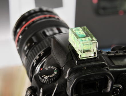
|
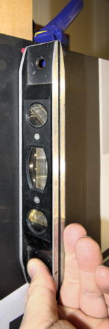 |
Rope trick (for horizontal positioning)
This trick uses rope and mirrors, as well as the red dots • tht mark the horizontal center of the target (or whatever marker you choose). This is as close to smoke and mirrors as Imatest gets.
The cord should be about 1 meter long and have a weight on one end. A heavy nut— the type that mates with a bolt, not the type that grows on trees— serves well.
Hold the cord in front of the camera (between the camera and mirror), and align your eye and the cord so the so the cord passes in front of the horizontal center markers (red dots • in the images), and so the reflection of the cord passes directly behind the cord. The camera is positioned properly if the center of the lens is aligned with the cord. If it isn't, shift the camera horizontally until it is.
To complete the horizontal adjustment, rotate (pan) the tripod pan/tilt head so the chart is centered in the image frame.
At this point you should be close enough to correct alignments so the final, fine adjustments should proceed quickly. |
 |
Other targets
The images below illustrate a problem that can arise using wide angle lenses. Glare appears in the outer patches, but it doesn't affect the critical outer edges. It's difficult to remove glare entirely: it can be impractical to place lights further from the target, and reducing the angle may make lighting too uneven. We have recently been dealing with glare by printing charts on high quality matte paper (Epson Ultra Premium Presentation - Matte), which resolves detail as fine as glossy and semigloss papers. Glare is rarely a problem with normal and telephoto lenses.
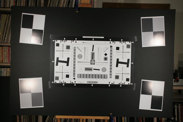
Modified ISO 12233 (QA-77) and slanted-edge charts
The QA-77 modified ISO chart, available from Applied Image, is printed on photographic media with higher resolution than is attainable with inkjet printers. It can be used with smaller image fields than inkjet-printed charts: valuable for close-up work and for analyzing telephoto lenses when space is limited. Note that the glare in the corner targets (no longer used) is doesn't affect the outer-most tangential edges. Careful positioning of lights is critical when working with wide-angle lenses.
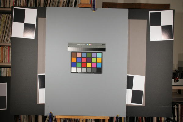
Kodak Q-14 Step chart and GretagMacbeth™ ColorChecker®
These charts (normally framed much closer) are analyzed with Imatest Stepchart, Colorcheck, and Multicharts. They are mounted on neutral middle gray (~18% reflectance) mat board, which is mounted on foam board for rigidity. Shown in front of the wider slanted-edge target. The Q-13/Q-14 can be mounted vertically to reduce glare when used with wide angle lenses.
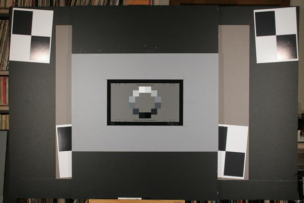
OECF target, available from Applied Image
The OECF target is valuable for measuring tonal response in cameras that have significant light falloff (vignetting)— especially for cameraphones, which are constrained to be extremely thin.
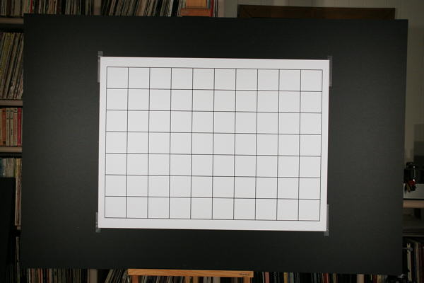
Distortion target, printed on an Epson 9800 inkjet
using a file generated by Imatest Test Charts
Additional targets: The veiling glare target is illustrated here.
Training
Two-day training
July 10-11 in Boulder, Colorado)
When: Thursday and Friday, July 10-11, 2008 | Where: Hotel Boulderado, Boulder, Colorado
Price: $1199
Students Will Learn How To:
- Measure key image quality factors using Imatest
- Understand and interpret Imatest output
- Avoid common mistakes in applying Imatest
- Select appropriate test charts
- Tailor Imatest options to target environments
- Assess overall image quality
|
|
|
Description: This
hands-on course provides the knowledge and skills needed
to effectively use Imatest and assess digital image quality. Students will learn the key factors that contribute to
overall image quality and how to apply Imatest to accurately measure
each factor. They will also learn how to
select appropriate test charts, configure Imatest options, and
interpret Imatest output. Small-group exercises will reinforce
learning and allow students to explore advanced image testing
techniques.
Day 1:
- Overview of key image quality factors
- Application of Imatest to measure key image factors
- Small-group exercises
- Discussion of results
Day 2:
- Advanced techniques and options for applying Imatest
- Understanding and interpreting Imatest output
- Small-group exercises
- Discussion of results
Instructor:
Norman Koren, inventor, founder of Imatest and primary author of Imatest software
For more information or to register over the phone, Contact Randy Bockrath, 720-235-2407,
.
| You may register using your credit card through PayPal. |
|
About Boulder: Located at the foot of the Rocky Mountains, 45 minutes from the Indian Peaks wilderness and just over an hour from Rocky Mountain National Park, Boulder has an outstanding variety of outdoor activities (especially hiking and bicycling) and cultural activities such as the Colorado Music Festival. For more, see Norman Koren's Boulder Visitor's Guide. The Hotel Boulderado offers a 20% discount for training participants. The Boulder University Inn, a short walk from the Boulderado, is a good budget alternative. Boulderlodging.com has a comprehensive list of lodgings.
Imatest Instructions
Installation
and getting started
Install Imatest
If you haven't dowloaded Imatest, go to the Imatest
download page before proceding. If you plan to install Imatest
on a computer that will not be conected to the Internet during
installation (or if you are behind a strong corporate firewall), download
the Matlab runtime library,
Imatest-lib.exe
(8.5 MB), to the same folder as the Imatest installer file. This only needs to be done on the initial installation, not for updates. If Imatest-lib.exe is not in this folder during installation, the installer attempts to download
it from the Internet.
You must have administrator priveleges on your computer during installation. This is rarely an issue, except on networked systems with strong security.
If
you have a strong personal firewall, you may need to disable it before you install
Imatest for the first time. You may re-enable it when the installation
is complete. This should not be necessary on subsequent installations.
Open Windows Explorer and double-click on the Imatest installer file, Imatest-version.exe.
(Version is the version number, 2.n.m. The Change Log contains the update history.) The version is displayed in the welcome window. Follow the instructions
in the installation wizard (mostly clicking
Next
>). The Imatest installation requires approximately 34 MB
(mostly the Matlab libraries).
When you install Imatest you agree to the terms of the Imatest license, which allows you to register and use the
software on (A) a maximum of three computers (for example, home, laptop,
and office) used exclusively by a single individual, or (B) a single workstation
used nonsimultaneously by multiple people, but
not both. It is not a concurrent use license. The full text of the license can be found here.
Imatest can be run by clicking the Imatest icon
on the Desktop, the Start menu, or in the Imatest installation folder (C:\Program
files\Imatest in English language installations). Instructions for running Imatest
are located in Imatest instructions.
Links to instructions for individual Imatest
modules are located in the Imatest Documentation
page.
If you encounter difficulties (usually caused by strong firewalls), make sure Imatest-lib.exe is in the same folder as the Imatest installer file. More details can be found on the Troubleshooting page.
When you first run Imatest,
it will be in evaluation mode, which allows up to 20 runs of individual
modules. Evaluation mode has all the capabilities of the registered
version except for two.
- It does not save results files.
- There is a watermark in the background of the plots.
You can upgrade to full unrestricted version by purchasing and registering Imatest.
Enhanced EXIF data acquisition
EXIF data is image file metadata that contains camera and lens settings. Selected EXIF data (important values such as aperture, exposure time, ISO speed, and focal length) is displayed in several figures and saved in CSV and XML output files.The jhead.exe program included in the standard Imatest installation can only read limited EXIF data from JPEG files. Imatest's EXIF acquisition capabilities can be greatly enhanced using Phil Harvey's ExifTool, which must be downloaded and installed separately from Imatest:
- Go to the ExifTool home page and download the Windows standalone executable (a zip file). This file is not included in the Imatest installation because it is frequently updated.
- In Windows Explorer, double-click on the downloaded zip file.
- Copy the contents ( exiftool(-k).exe ) to the Imatest installation folder (typically C:\Program files\Imatest in English-language installations).
- Rename exiftool(-k).exe to exiftool.exe.
- Make the approprite selection in the Exif Data Acquisition area of Options & Settings II. More details here.
Purchase
Imatest
You may purchase Imatest at any time from Imatest's online store. You will be entitled to updates for one year from the date of purchase. After one year you will need to renew your subscription to install new upgrades.
You can also click on the Purchase
button in the Imatest main window.
After you purchase Imatest you'll receive an e-mail confirmation
of your purchase.
This may take a few minutes. You may register Imatest as soon as you receive
this e-mail; the password is the same one you used to sign up to Imatest.com.
If you don't receive the email within about fifteen minutes, contact us.
Register
imatest
After you've installed and purchased Imatest or Imatest Renewal you'll need to register it by clicking on the Register button in the Imatest main window or by clicking on Help, Register. It's a good idea to check the Imatest
download page or Change log for the latest version.
If
you have a personal firewall, be sure to disable it before you register.
You may re-enable it as soon as registration is complete. If you can't disable it or you can't register following the instructions below, try Offline registration.
You must have administrator priveleges on your computer. This is rarely an issue, except on networked systems with strong security.
Fill in the the Register Imatest
window: Enter your name, company (if applicable), e-mail, and the password
you entered when you signed up on Imatest.com, then click on Register.
If you forgot your password, click on Recover
password. This opens a web page that enables you to recover your lost password via e-mail.
If your computer is connected to the internet, you will receive a confirmation of your registration. The version of Imatest you purchased (Light or Pro) will be activated immediately. In rare instances where the pressing Register hangs up the computer, click on Manual activation and follow the instructions below.
Offline registration
If your computer is offline, or if you are unable to connect because
of a firewall that can't be disabled, the following box appears in response to Register.
Click on Offline activation. The box below appears with instructions
for offline (manual) registration. Steps 2-4 can be performed on any computer connected
to the internet.
On www.imatest.com/activate, fill in all the fields as shown below, then click Make Activation Code . Don't leave any fields blank— always enter something. Your code will be e-mailed to you. Enter it into the Activation key: field, above.
Reminder: For offline installation, the Matlab runtime library,
Imatest-lib.exe (8.5 MB), must be downloaded to the same folder as the Imatest installer file. If you have difficulties, refer to the Troubleshooting page.
Files
When the installation
is complete the Imatest folder should contain the following folders and
files.
The default installation
folder for Imatest is C:\Program files\Imatest.
(It may differ in non-English
installations.)
.
| samples (folder) |
Contains several image files
with sample data for testing the three Imatest modules. Includes
several
cropped JPEG files for testing SFR, indicated by _sfr in their names.
Canon_EOS10d_ColorCheck_lt_small.jpg — for testing Colorcheck.
Canon_EOS10D_Q13_ISO400_small.jpg — for testing Q-13.
Edge_chart.png and Edge_chart_low.png — the printable SFR edge images.The latter
(low contrast) is recommended.
|
| images (folder) |
Contains several image files
used by Imatest. |
| bin (folder) |
Contains the .fig files
used in the graphic user interface (GUI), as well as Matlab library files.
Includes FigureMenuBar.fig and FigureToolBar.fig: library files missing
from Imatest-lib.exe. |
| toolbox (folder) |
Subdirectories contain Matlab
library files (mostly DLLs). |
|
Imatest |
(full name Imatest.lnk)
The standard icon for running Imatest. Runs start.bat, which sets the path
then runs imatest.exe. Copied to Windows Start Menu and Desktop. |
|
Diagnoistics |
(full name Diagnostics.lnk)
Runs Imatest in diagnostic mode. Doesn't close when Imatest terminates.
This allows error messages to be viewed. Runs diagnostics.bat, which sets
the path then runs imatest.exe. |
| jhead.exe |
DOS application for reading
EXIF data (digital camera information). |
| dcraw.exe |
Dave Coffin's dcraw RAW conversion program. |
| imatest.exe |
Imatest executable program. |
start.bat
imadiag.bat |
Batch files that set the
Windows Path and run Imatest.exe. Diagnostics.bat is used for diagnostic
mode: the DOS window remains open if Imatest terminates with an error. |
| License.txt |
The Imatest End User License Agreement (EULA) |
The Imatest License
The Imatest license for Light and Pro allows an individual user to register and use the software on (A) a maximum of three computers (for example, home, laptop, and office) used exclusively by a single individual, or (B) a single workstation used nonsimultaneously by multiple people, but not both. It is not a concurrent use license.
License holders are encouraged to publish test results in printed publications, websites, and discussion forums, provided they include links to www.imatest.com. You may not use Imatest for advertising or product promotion without explicit permission from Imatest LLC. Contact us if you have questions. The full text of the license can be found here.
Using Imatest
Running Imatest
Imatest is opened by double-clicking the Imatest icon on
- the Desktop,
- the Windows Start menu ( Start → All Programs →Imatest → Imatest ),
- or the Imatest directory (usually C:\Program files\Imatest in English language installations).
| |
To run Imatest in Windows Vista, you'll need version 2.3.3 or later. |
After several seconds, the Imatest main window, shown below, opens. Imatest modules are run by clicking on one of the buttons on the left. Instructions for the individual modules are on their own pages, listed below. Click here for the documentation Table of contents.
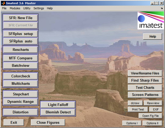
Imatest main window
When you first install Imatest it operates in evaluation mode, which allows 20 runs and does not allow data to be saved. A welcome page summarizing Imatest's capabilities and operations is displayed when Imatest is started in evaluation mode. To continue using Imatest you must purchase and register it.
 Font size/DPI scaling issue Font size/DPI scaling issue
If DPI scaling is set to Larger scale (120 DPI), buttons at the top and the right of the Imatest main window may be truncated. This problem should be fixed with Imatest 3.2.1. In earlier versions there are two fixes.
1. In the Imatest main window, click Settings (on the top bar), Enlarge screen.
2. (In Vista) Right-click on the wallpaper, click on Personalize, then click on Adjust Font size (DPI) (near the top of the left bar) to open the DPI scaling window. Select Default scale (96 dpi) instead of Larger scale (120 dpi). Reboot for the change to take effect. |
The following steps are typical for most Imatest modules.
-
Open the image file. A dialog box requests the name of the input image file. Imatest supports
TIFF (24 or 48-bit; without LZW compression), JPEG, PNG (24 or 48-bit), BMP, HDF, PCX, XWD, and PPM (24 or 28-bit) file
formats. It also supports RAW files for a large variety of digital cameras, using Dave Coffin's dcraw. New cameras are typically added to dcraw within a month or two of their introduction. The dcraw page has the latest list of cameras.
Multiple file read
In Imatest Master you can select several files to read.
Depending on how you respond to the multi-image dialog box (below),
- The files can be analyzed individually in sequence (batch mode), or
- The files can be combined— averaged— and the mean analyzed (it can also be saved). This is useful for measuring sensor fixed pattern noise in Stepchart, Colorcheck, and Light Falloff and in SFR for measuring performance of image stabilization.
The files should be in the same folder, have the same pixel dimensions, and be framed identically. If you choose Combine files, you'll have the option of saving the combined file with 16-bit TIFF format as default. Batch mode is not supported in Rescharts.
The saved file name is the same as the first selected file name with _comb_n appended, where n is the number of combined files. |
- Enter additional input data. Unless Express mode has been selected, a dialog box opens that requests the title (which defaults to the file name)
and other data, depending on the module. Most additional data is optional (most is saved from previous runs); you only need to pay attention to settings you wish to change. Click OK to continue or Cancel to terminate
the run.
- Run the program by clicking OK. The results are presented in individual Figures.
- Save results? A dialog box asks if you would like to save the results. Checkboxes in
the dialog box enable you to select the Figures and .CSV (Excel-readable) and XML files to be saved. You may examine
the results before deciding which, if any, to save. (The Save box is omitted in the evaluation version.)
About RAW files
RAW files are the unprocessed output of digital image sensors. For Bayer sensors, each RAW pixel represents a single color in RGRGRG, GBGBGB, ... sequence. To be converted into usable, standard file formats (TIFF, JPEG, etc.), raw files must be processed by a RAW converter. RAW converters perform several functions: demosaicing (converting the Bayer sequence into full color), applying a gamma curve, often with an additional tonal response curve, reducing noise, and sharpening the image. These operations can affect Imatest's measurements, especially SFR.
More detail can be found in RAW files.
|
dcraw input dialog box
|
The best way to be sure an image file faithfully resembles the RAW file— that it has a pure gamma curve, no sharpening, and no noise reduction— is to read a RAW file into Imatest and convert it into a standard format (typically TIFF) using Dave Coffin's dcraw. If you select any of the standard RAW formats (CRW, NEF, etc.) or if a file that contains RAW data (e.g., Phase One TIF) is detected the dialog box on the right appears. It allows you to choose among several RAW conversion options.
dcraw conversion details:
You can select normal raw conversion (with demosaicing) or 8 or 16-bit Bayer raw (RGRGRG, GBGBGB, ... sequence; undemosaiced). The latter formats allow several Imatest Master modules to examine the unprocessed pixels. Choices:
| Demosaicing |
Normal RAW conversion (demosaiced) |
| RAW 8-bit (Bayer RAW; no demosaicing) |
| RAW 16-bit (Bayer RAW; no demosaicing) |
You can choose among three conversion programs (all based on dcraw).
| Program |
dcraw |
The original; may not work in Vista |
| LibRaw |
dcraw emulator (works in Vista; no Bayer RAW) |
| dcrawMS |
Works in Vista |
The following output color spaces are available for demosaiced output.
RAW (not true RAW pixels):
Demosaiced with no color space conversion or White Balance.
The camera's color profile is needed to correctly interpret the colors. Gamma = 0.45. |
| sRGB, Adobe RGB (1998), Wide Gamut RGB, ProPhoto RGB, and XYZ. |
Profile tags are embedded in the output file for the four standard color spaces. For 24-bit conversion, gamma appears to be fixed at 0.45, independent of the output color space. (It should be different for ProPhoto, which is designed for display at gamma = 1.8.) For 48-bit conversion gamma is fixed at 1 (linear conversion; does not correspond to standard color spaces).
Auto-exposure is always applied for 24-bit conversion (but not for 48-bit). I've changed the default to make it slightly darker than the dcraw default (using -b 0.99 in the command line) to reduce the likelihood of clipping pixels. For now we're stuck with auto-exposure for 24-bit conversion: see dcraw Frequently Asked Questions.
Dcraw converts RAW files into TIFF files. (The obscure PPM format is available as an option.) If check the box to delete the converted (TIFF) file, you may save the image in one of two compressed formats: PNG (lossless compression; takes longer) or JPEG (lossy compression; maximum quality; 24-bit only).
A list of supported cameras appears on the dcraw site. New cameras are typically added within one to three months of their introduction. The dcraw version included with Imatest sometimes falls behind. According to Dave Coffin, "Francisco Montilla provides Mac OS and Windows executables on his website. And Benjamin Lebsanft has volunteered to maintain Windows executables optimized for specific CPUs."
|
Dcraw does not currently run on Windows Vista. According to the dcraw FAQ, it should work when Service Pack 1 (SP1) is released. |
|
Miscellaneous controls
Exit closes all figures and terminates Imatest.
Close figures closes all figures. You can close figures individually by the usual Windows methods — clicking
the X in the upper right or
right-clicking on the figure icon on the Taskbar and selecting Close.
Saved settings: Imatest saves a number of settings, including Font size, folders for opening and
saving images (for all modules), plot selection (for SFR), and figures to save. To restore these settings to their
original defaults, click the Settings menu
(in the toolbar on the top of the Imatest window), then click Reset defaults, Yes. The settings are stored in Imatest.ini.
Options I... and Options II... (at the bottom of the Imatest main window to the left of the Fonts menu); also in the Settings dropdown menu) opens the boxes shown below, which allow several options to be specified.
Options I
Options I for setting ROI options, Large file processing, and Batch run order.
Expert vs. Basic mode affects the complexity of input dialog boxes. Basic (beginner) mode uses a simplified dialog box and uses defaults for settings that are not displayed. Modules are gradually being added.
ROI (Region of Interest) section controls cropping options.
- SFR ROI filtering When Light filtering is checked the tests that validate the SFR ROI (region of interest) are relaxed. This can be useful when testing noisy images, rough edges, images of endoscopes or other devices with interfering patterns, but it can lead to errors if regions are selected carelessly. Normal filtering is the default.
- Stepchart ROI selection Automatic selection (the default) can be toggled. If it is turned off, a fixed number of patches (6-41) can be selected for Stepchart analysis. This option is useful when high noise in dark regions confuses the automatic ROI detection.
- Colorcheck, Distortion, Light Falloff Cropping options. You can select whether to ask for cropping and whether to use the last crop (for same-sized images). For Colorcheck you can also choose between traditional automatic patch detection and Multicharts-like patch detection, where all squares are shown in the fine adjustment window.
LARGE FILES (Light Falloff, Distortion) These two modules typically use little or no cropping. As a result, memory may sometimes overflow. This setting offers the option of cutting the image dimensions in half (1/4x in area and memory) to avoid memory problems.
Batch run order The actual order of batch runs may differ from the order of selection in curious ways that depend on the operating system or other factors. With one of the choices in this popup menu the run and selection orders should be the same.
Reset restores defaults: it sets SFR ROI filtering to Normal, Stepchart ROI selection to Automatic, turns off all global folder settings, and checks Get EXIF data .
Options II
Options II for setting folder options, SFR save file suffix, etc.
Global folders The default folders for opening files and saving results can be set globally using the second group of controls. Normally (with Global folder for opening files unchecked), the default folder for opening files is changed only for the Imatest module in use: one module at a time. When it is checked, the default folder for opening files is changed for all modules. This can be convenient if project data for several modules is stored in the same file.
When either of the Global folder for saving results... radio buttons is set, the default save folder is changed for all modules whenever the input folders are changed.
EXIF data acquisition This selects the program used to read EXIF data: image file metadata that contains camera and lens settings. Selected EXIF data (important values such as aperture, exposure time, ISO speed, and focal length) is displayed in several figures and EXIF data is saved in CSV and XML output files. There are four settings:
| 1 |
Get EXIF data from jhead.exe (default; JPEG-only, limited) |
Default |
| 2 |
Get EXIF data from Phil harvey's ExifTool (all file types; must download & install) |
Recommended |
| 3 |
Get EXIF data from ExifTool & save ALL EXIF data in csv output (LOTS)! |
Detailed! |
| 4 |
Do not get EXIF data (for rare cases of errors) |
EXIF off |
Setting 1, jhead.exe, is the default. Jhead is a compact program with limited capabilities included in the Imatest installation file. It only works with JPEG files, and it captures limited EXIF data. Settings 2 and 3 (ExifTool; introduced with Imatest 3.2.1) work with virtually any file type and capture virtually all available EXIF data. If the setting 3 (save ALL EXIF) is selected, all the EXIF data— a huge amount; some quite obscure— is written to the CSV output files.
The second and third settings require that ExifTool be downloaded and installed.
- Go to the ExifTool home page and download the Windows standalone executable (a zip file). This file is not included in the Imatest installation because it is frequently updated.
- In Windows Explorer, double-click on the downloaded zip file.
- Copy the contents ( exiftool(-k).exe ) to the Imatest installation folder (typically C:\Program files\Imatest in English-language installations).
- Rename exiftool(-k).exe to exiftool.exe.
The final selection is for very rare cases (e.g., industrial prototypes with non-standard EXIF data) that cause the EXIF read routine to crash.
Suffix for saved SFR plots and CSV and XML files Normally the root name (input or selected file name ) is followed by the channel, ROI orientation (AL = above left (relative to the center), etc.) and distance from the center in percentage of distance to the corner. Example: rootname_YAL79_MTF.png for the Edge/MTF plot. An alternative can be selected where _ROI_ followed by the ROI number nn is used in place of the orientation and distance. Example: rootname_ROI_03_MTF.png
Special user code enables custom features for specific users. Normally blank.
Reset restores defaults: it sets SFR ROI filtering to Normal, Stepchart ROI selection to Automatic, turns off all global folder settings, and checks Get EXIF data .
Help opens a relevant web page on computers connected to the Internet.
Dropdown menus
Dropdown menus are located at the top of the Imatest main window. Most items duplicate the controls elsewhere in the window, but some are unique.
File contains Clear Memory, Close Figures, and Exit. Clear Memory removes the image data stored after running SFR. This may release enough memory to speed up other modules, such as Light Falloff, which can use large amounts of memory.
Modules opens the Imatest modules. The entries duplicate the buttons on the left of the Imatest main window.
Settings contains functions that control various aspects of Imatest operation.
- Small / Normal / Large fonts alters the font size in output
figures and GUI windows. The default is Normal.
The setting is saved between runs. This address problems with tiny fonts in high resolution
screens (1600x1200 pixels and above)
or larger than expected fonts which appear when the video card DPI setting
is Large size (120 DPI) instead of Normal. The video card setting can be accessed by
right-clicking on the Windows background, then clicking Properties, Settings,
Advanced, General (tab). Large fonts are displayed if DPI is set to Large size (120
DPI). 96 DPI is normal. Windows may need to be rebooted
before new settings take effect.
- Save Settings copies settings from imatest.ini (which stored the current, active settings) to a named file (with extension ini). Particularly useful for saving regions of interest (ROIs) for SFR runs and for controlling Imatest API modules. The most recent folder used to save or retrieve settings is displayed in the file selection dialog box, but any folder may be selected.
- Load Settings retrieves settings from a named file (with extension ini) and stores them in imatest.ini. It is useful for restoring ROIs or for restoring settings after they have been reset. The most recent folder used to save or retrieve settings is displayed in the file selection dialog box, but any folder may be selected.
- View Settings displays the settings— the contents of imatest.ini— in the Notepad viewer. You can edit this file (with care!) and save it as a named file if desired. You can send us the contents of imatest.ini for help with troubleshooting. The Notepad window should be closed when you are finished viewing it: it may interfere with some Imatest operations.
- Reset defaults restores settings to their default values by resetting imatest.ini. On rare occasions this clears bugs. See Troubleshooting. It is a good idea to save settings prior to resetting them.
- Edit/reset module(s) opens a special editor that allows ini file values to be examined and entire sections to be deleted if the corresponding module crashes. Described in Troubleshooting.
- Options and settings I and II contain settings that affect SFR ROI (region of interest) error checking, Stepchart ROI selection, and folder names for storing results, and more.
- DOS command allows you to enter a DOS command while Imatest is running. Useful for troubleshooting, for example, for diagnosing path issues.
- When checked, Fixed sharpening radius keeps the SFR standardized sharpening radius fixed, even for edges with poor MTF where it would otherwise automatically increase.
- API options sets several options for controlling API runs.
- Enlarge hi res figs applies only to high resolution screens (1600x1200 pixels and above). When this box is checked (by default), images are enlarged so they don't look tiny on the screen. Unchecking the box turns this feature off. Images are smaller but better suited for website presentation. The setting is saved.
Help contains Online Help, Register, Register Upgrade, and About, and Welcome window.
- Online Help corresponds to the Help button; it opens a browser window.
- Register and Register Upgrade is used to register Imatest.
- About displays the Imatest version and user registration information.
- Welcome window displays the window that normally appears when Imatest is started in evaluation model.
Figures
Imatest results are displayed in individual windows called figures.
A typical figure— the result of running SFR for the Canon EOS-10D— is
shown below.
|
Figures
may be resized, minimized, maximized, or closed using standard Windows
operations. In addition, several Windows and Matlab-specific operation
can be found in the toolbar at the top of the image.
The first four icons
in the toolbar are standard Windows icons: New file, Open, Save, and Print.
Open and Save refer to Matlab .fig figures, which can only be opened from
the Matlab program or a Matlab figure window. Imatest allows you to save figures as PNG files— an excellent format with lossless
compression.
Of the remaining three icons, the most useful is Zoom
in:  .
Clicking on it highlights it and enables you to zoom in on regions of the
plots. You can click and drag to create a zoom rectangle or you can click
on any point to zoom in on that point. Double-clicking anywhere on the image
restores the magnification to its initial state .
Clicking on it highlights it and enables you to zoom in on regions of the
plots. You can click and drag to create a zoom rectangle or you can click
on any point to zoom in on that point. Double-clicking anywhere on the image
restores the magnification to its initial state |
Imatest figure: You can resize it or zoom in on individual plots.
|
Two precautions when working with Figures
|
Too many open Figures
Figures can proliferate if you do a number of runs, especially SFR runs with multiple regions,and
system performance suffers if too many Figures are open. You will need to manage them. Figures
can be closed individually by clicking X on the upper right of the
Figure or by any of the usual Windows techniques. You can close them all
by clicking Close figures in the Imatest main window.
|
Clicking on Figures during calculations
Plots can appear on the wrong figure (usually distorted) or disappear altogether.
Wait until all calculations are complete— until the Save or Imatest main
window appears— before clicking on any Figures.
|
To see Figure resource use, open the Windows Task Manager. In Windows XP, click
Control-Alt-Del or right-click in the Taskbar, usually at the bottom of
the screen. Click on the Processes tab, then click CPU twice so the tasks
with the most CPU usage appear at the top. Imatest can be a real CPU hog when several Figures are open; CPU use appears to increase with the
square of the open Figures. On my dual 1 GHz Pentium Windows XP machine,
8 open Figures use 6% of the CPU; 16 open Figures use 33%. Over 20 would
seriously slow the computations.
.CSV and XML output files
Individual Imatest modules can optionally write two types of output file, which contain most of the results. They may, if desired, be entered into other programs. .CSV files are most often displayed with Microsoft Excel. XML files can be used as input to database programs and for additional applications yet to be developed. They can be displayed in somewhat readable form with any web browser. Please contact us if you have requests or suggestions about Imatest output. Note: These files are not saved in evaluation mode.
CSV files– Excel-readable Comma-Separated Variable format. Here is an example of typical output.
Module,Colorcheck
File,Canon_EOS10d_ColorCheck_lt_small.jpg
Run date,31-Dec-2005 18:11:00
Zone,Gray,Pixel,Pixel/255,Px/255 ideal,Log(exp),Log(px/255),WB Err Deg,WB Err Mired
19, 1, 241.6, 0.9475, 0.9569, -0.050, -0.023, 163, -3.8
20, 2, 215.8, 0.8464, 0.7922, -0.230, -0.072, 491, -10.8
21, 3, 179.0, 0.7020, 0.6353, -0.440, -0.154, 450, -10.0
The same data displayed in Excel looks like this.
XML files– Similar output to the .CSV data above is shown below, displayed in the Firefox browser, which formats the results slightly (adds indentation and colors). XML output was introduced with Imatest 1.6.4. It will be refined in succeeding releases.
Use of Imatest
The Imatest license for Light and Pro allows an individual user to register and use the software on (A) a maximum of three computers (for example, home, laptop,
and office) used exclusively by a single individual, or (B) a single workstation
used nonsimultaneously by multiple people, but
not both. It is not a concurrent use license.
License holders are encouraged to publish test results in printed publications,
websites, and discussion forums, provided they include links to www.imatest.com.
The use of the Imatest Logo is encouraged. However you may not use Imatest
for advertising or product promotion without explicit permission from
Imatest LLC. Contact us if you have questions.
The full text of the license can be found here.
Imatest LLC assumes no legal liability for the contents of published
reviews. If you plan to publish test results, especially for MTF, you should take care to use
good technique. Considerations include,
| Sturdy camera support |
Use a sturdy tripod, cable
release, and, if possible, mirror-lock. |
| Target mounting |
If you are working outdoors,
be sure the target doesn't shake in the wind. |
| Target distance |
Be sure you're far enough
from the target so the printed edge quality doesn't affect the measurements.
Target distance considerations are given
here. |
| Focus |
Be sure the camera is focused
accurately on the target. Note whether you used manual or automatic focus. |
| Target alignment |
Make sure the corners, as
well as the center, are in focus. |
| Illumination |
Should be as even as possible. |
| Exposure |
Take care not to clip shadows or highlights. This will reduce accuracy of the results. |
| Raw conversion and settings |
The choice of RAW converter
(in or out of the camera) and settings, particularly Sharpening, can make a
huge difference. Contrast
and White balance are also important. Settings that affect contrast and
transfer curve can also have a strong effect. If possible a "Linear" setting (meaning a straight gamma curve with no additional tonal
response adjustments) should be used. |
Gamma
|
SFR
sharpness results are moderately sensitive to the Gamma setting: A 10%
gamma error changes MTF50 by 2.5%. For best results gamma should be
measured by running Colorcheck or Stepchart. Ideally a Q-14 target (similar to the Q-13, but larger) should be mounted close to the slanted edge images. |
| Cleanliness and filters |
Lens surfaces should be
clean. You should note whether you have a protective (UV or Skylight) filter.
It can make a difference— more likely reduced contrast than reduced sharpness.
With Imatest you can find out. |
| File formats |
Use RAW or the highest JPEG
quality. Never use less than the maximum resolution or JPEG
quality unless you are specifically testing the effects of these settings. |
| Lens settings |
Lens performance is a strong
function of the aperture (f-stop) and focal length (for zooms). Be
sure to record these settings (easy because they're saved with the EXIF
data) and include them in your writeup. The optimum (sharpest) aperture
is of particular interest. Lens performance is also somewhat affected by
the distance to the target. |
| White balance |
Should be close as possible
to neutral, particularly in Colorcheck. |
This
may seem like a lot of fuss, but the technique you develop in
testing cameras and lenses will spill over to your daily photography. Alfred
Stieglitz tested film and developers extensively when he discovered photography
as a student in Berlin. Ansel Adams performed extensive tests in the development
of his zone system. Although nobody would claim that testing is responsible
for their unique vision, it certainly contributed to the skill that transformed their vision into prints of transcendent beauty.
RAW files
Bayer RAW support:
Imatest 2.7.1
SFR, Stepchart, and all Rescharts modules (SFR, Log Frequency, Log F-Contrast, and Star chart) all support Bayer RAW files.
Light Falloff is the most important module that does not yet support it. |
RAW files
The unprocessed digital output of an image sensor is called a RAW file. In this document we sometimes refer to it as Camera RAW to distinguish it from Bayer RAW files, which are standard image files that contain undemosaiced (Bayer) data.
The pixels in most digital image sensors are covered with a Bayer Color Filter Array (CFA), which makes each pixel sensitive to a single primary color, Red, Green, or Blue. The order of the colors is RGRGRG..., GBGBGB..., etc. There are twice as many greens as reds or blues because the eye is most sensitive to green. The four possible pixel arrangements (Red locations) are shown in the diagram below, where pixel locations start with Row 1 Column 1 (R1C1) in the upper left corner. There is no univesal standard for mapping colors (R, G, or B) to pixel position (RmCn) in RAW files. The arrangement can be determined by examining a Bayer RAW image file with the Rawview utility, which can be called from a button on the right of the Imatest main window.
R1C1
|
R1C2
|
R1C3
|
R1C4
|
R2C1
|
R2C2
|
R2C3
|
R2C4
|
R3C1
|
R3C3
|
R3C3
|
R3C4
|
R4C1
|
R4C2
|
R4C3
|
R4C4
|
Red in R1C1 |
R1C1
|
R1C2
|
R1C3
|
R1C4
|
R2C1
|
R2C2
|
R2C3
|
R2C4
|
R3C1
|
R3C3
|
R3C3
|
R3C4
|
R4C1
|
R4C2
|
R4C3
|
R4C4
|
Red in R1C2 |
R1C1
|
R1C2
|
R1C3
|
R1C4
|
R2C1
|
R2C2
|
R2C3
|
R2C4
|
R3C1
|
R3C3
|
R3C3
|
R3C4
|
R4C1
|
R4C2
|
R4C3
|
R4C4
|
Red in R2C1 |
R1C1
|
R1C2
|
R1C3
|
R1C4
|
R2C1
|
R2C2
|
R2C3
|
R2C4
|
R3C1
|
R3C3
|
R3C3
|
R3C4
|
R4C1
|
R4C2
|
R4C3
|
R4C4
|
Red in R2C2 |
Most camera RAW formats are proprietary to the camera manufacturer (e.g., CR2 for Canon and NEF for Nikon) and must be converted into standard file formats (JPEG, TIFF, PNG, etc.) for most applications. This usually involves demosaicing, which is a form of interpolation that fills in the two missing colors in each pixel. Demosaicing is the primary function of RAW converter programs (which may be either built into the camera or implemented on a separate computer). In demosaicing, detail in the missing colors is inferred from detail in other, neighboring colors. Algorithms can be very mathematically sophisticated. Demosaicing (RAW conversion) programs usually incorporate a number of secondary image processing steps, including
- applying a gamma curve, typically with a tonal response curve often applied on top of it,
- white balance and color adjustment,
- sharpening, usually in the neighborhood of contrasty features, and
- software noise reduction, typically in the absence of contrasty features.
All these steps can affect Imatest results. To minimize their effects, Imatest uses dcraw, a freely available program for converting RAW images to useful file formats. Dcraw applies simple gamma curves (with no additional tonal response curves) and does not perform sharpening or noise reduction.
RAW files in Imatest
Imatest can use RAW files in two ways. Both use dcraw.
- It can demosaic RAW files, producing standard 3-color RGB image files in TIFF, PPM, PNG, or JPEG format, with TIFF as the default. The advantage of using dcraw is that it applies no sharpening, no noise reduction, and a straight gamma curve (gamma = 0.45 for 24-bit output files or 1.0 for 48-bit files). If RAW files are available, cameras and lenses from different manufacturers can be compared on a consistent, fair basis.
Dcraw should be used with caution in Colorcheck and Stepchart because is performs autoexposure for 8/24-bit output. According to the dcraw FAQ, "No matter how dark an image is, dcraw's auto-exposure stretches it so that one percent of its pixels appear white. The "-b" option adjusts this behavior, while "-4" (16-bit output) avoids it entirely."
- It can convert camera RAW files into Bayer RAW files stored in standard monochrome image file formats (TIFF or PGM). Starting with version 2.6.4 several Imatest Master modules (SFR, Rescharts, and Stepchart, with more on the way) can analyze Bayer RAW files.
Bayer RAW is particularly valuable for measuring lateral chromatic aberration, which can be strongly distorted by the demosaicing process.
|
Dcraw does not currently run on Windows Vista. According to the dcraw FAQ, it should work when Service Pack 1 (SP1) is released. However, DcrawMS in Imatest 3.2 works with Vista. |
To use RAW files in Imatest, either
- Click on an Imatest module (SFR, Stepchart, etc.) and open the file just as you would any other image file. If a camera RAW image file (CR2, NEF, etc.— even Phase One RAW TIF files) is detected, the dialog box shown on the right for setting dcraw parameters is opened.
- Click on the dcraw box on the right side of the Imatest main window (or click Modules, Run dcraw) to run dcraw as a standalone application: the output file will be saved but no Imatest module will run. The dialog box on the right is a graphic user interface (GUI) front-end to dcraw that allows you to select several of dcraw's options.
|
dcraw dialog box |
Dcraw can either (A) demosaic camera RAW files with minimal processing— no sharpening, no noise reduction, and a simple gamma curve, or (B) convert them to standard 8 or 16-bit monochrome file formats (TIFF or PGM) that contain Bayer RAW (undemosaiced) data, which can be analyzed by several Imatest Master modules. This conversion has the following choices:
| Demosaicing |
Normal RAW conversion (demosaiced) |
| RAW 8-bit (Bayer RAW; no demosaicing) |
| RAW 16-bit (Bayer RAW; no demosaicing) |
If the second or third option above (RAW 8-bit or RAW 16-bit) is selected, the Demosaicing area (above) is grayed out and the output of dcraw is a monochrome TIFF or PGM file that contains undemosaiced (Bayer RAW) data from the image sensor. Three separate dcraw programs are available.
| Program |
dcraw |
The original; may not work in Vista |
| LibRaw |
dcraw emulator (works in Vista; no Bayer RAW) |
| dcrawMS |
Works in Vista |
DCrawMS.exe is a special build of dcraw designed to work with Vista. If you have a recent camera that doesn't work with dcraw or dcrawMS, try downloading the latest versions from Pukkita's Digital Darkroom Corner to the Imatest installation folder (C:\Program files\Imatest in most English language installations). LibRaw is a DLL library based on dcraw.
Bayer RAW files
Whenever a monochrome file is opened by an Imatest Master module that supports Bayer RAW, the dialog box shown on the right appears. Standard monochrome file should be selected for regular monochrome files that do not contain Bayer RAW data. The color scheme of the buttons depends on the "Red in RmCn" selection, which affects some of the displays. The correct setting can be found using the Rawview utility.
|
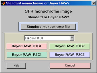 |
If Bayer RAW R1C1, R1C2, ... is selected, one of the four image planes starting with R1C1 (Row 1 Column 1), R1C2, R2C1, or R2C2 is selected for analysis. (Recall that there is no universal standard mapping an image plane with a color.) The four planes are shown below. Note that the pixel height and width of the image in each plane is half that of the image as a whole and the spacing between pixels is twice that of the sensor pixel spacing.
R1C1
|
R1C2
|
R1C3
|
R1C4
|
R2C1
|
R2C2
|
R2C3
|
R2C4
|
R3C1
|
R3C3
|
R3C3
|
R3C4
|
R4C1
|
R4C2
|
R4C3
|
R4C4
|
↓
R1C1
↓
|
R1C1
|
R1C2
|
R1C3
|
R1C4
|
R2C1
|
R2C2
|
R2C3
|
R2C4
|
R3C1
|
R3C2
|
R3C3
|
R3C4
|
R4C1
|
R4C2
|
R4C3
|
R4C4
|
↓
R1C2
↓
|
R1C1
|
R1C2
|
R1C3
|
R1C4
|
R2C1
|
R2C2
|
R2C3
|
R2C4
|
R3C1
|
R3C2
|
R3C3
|
R3C4
|
R4C1
|
R4C2
|
R4C3
|
R4C4
|
↓
R2C1
↓
|
R1C1
|
R1C2
|
R1C3
|
R1C4
|
R2C1
|
R2C2
|
R2C3
|
R2C4
|
R3C1
|
R3C2
|
R3C3
|
R3C4
|
R4C1
|
R4C2
|
R4C3
|
R4C4
|
↓
R2C2
↓
|
The four image planes: one Red, one Blue, two Greens:
(There is no universal standard mapping colors to image plane.)
Demosaiced files
The best way to be sure an image file faithfully resembles the RAW file— that it has a straight gamma curve, no sharpening, and no noise reduction— is to read a RAW file into Imatest and convert it to a standard format (TIFF, PPM, etc.) using Dave Coffin's dcraw. If you select any of the standard RAW formats (CRW, NEF, etc.) or if raw data is detected (e.g., Phase One TIF files) the dialog box shown above appears. It is a front-end to dcraw that allows you to choose between several RAW conversion options.
dcraw/dcrawMS conversion details:
If Normal RAW conversion (demosaiced) has been selected, the Demosaicing box contains several options, most of which are explained in more detail in the dcraw Manpage. The following output color spaces are available for demosaiced output.
RAW (not true RAW pixels).
Demosaiced with no color space conversion or White Balance.
The camera's color profile is needed to correctly interpret the colors. Gamma = 0.45. |
| sRGB, Adobe RGB (1998), Wide Gamut RGB, ProPhotoRGB, and XYZ. |
Profile tags are embedded in the output file for the four standard color spaces. For 24-bit conversion, gamma appears to be fixed at 0.45, independent of the output color space. (It should be different for ProPhoto, which is designed for display at gamma = 1.8.) For 48-bit conversion gamma is fixed at 1 (linear conversion; does not correspond to standard color spaces). Several demosiacing quality levels (using different algorithms) are available (and worth exploring). See the dcraw Manpage for details.
Auto-exposure is always applied for 24-bit conversion (but not for 48-bit). I've changed the default to make it slightly darker than the dcraw default (using -b 0.99 in the command line) to reduce the likelihood of clipping pixels. For now we're stuck with auto-exposure for 24-bit conversion: see dcraw Frequently Asked Questions.
Dcraw converts RAW files into TIFF files, with the obscure PPM format available as an option. If check the box to delete the converted (TIFF) file, you may save the image in one of two compressed formats: PNG (lossless compression; takes longer) or JPEG (lossy compression; maximum quality; 24-bit only).
A list of supported cameras appears on the dcraw site. New cameras are typically added within one to three months of their introduction. The dcraw version included with Imatest sometimes falls behind. According to Dave Coffin, "Francisco Montilla provides Mac OS and Windows executables on his website. And Benjamin Lebsanft has volunteered to maintain Windows executables optimized for specific CPUs."
Rawview utility
The Rawview utility allows you to determine the color arrangement of Bayer RAW files (Red in R1C1, R1C2, R2C1, or R2C2) by trying each and selecting the one that looks best. It can be opened by pressing the Rawview button on the far right of the Imatest main window, just to the right of dcraw. When Rawview is first opened, instructions similar to those shown below appear. (They are likely to be more up-to-date.)
Welcome to Rawview. Preview Bayer RAW files.You can find the relationship between colors and pixel locations.
The input file should be a monochrome file (r x n x 1 pixels) that contains Bayer Raw data.
The image is not fully demosaiced: it has only half-resolution.
There is no White Balance. Colors may appear faint.
16/48 bit images are lightened to improve visibility.
The input image should have some strong, identifiable colors.
Start by pressing "Read (Bayer) RAW image file."
Click on "Red in RmCn..." popup menu and determine which selection looks correct. |
After the image file has been read, the Rawview window looks like this:
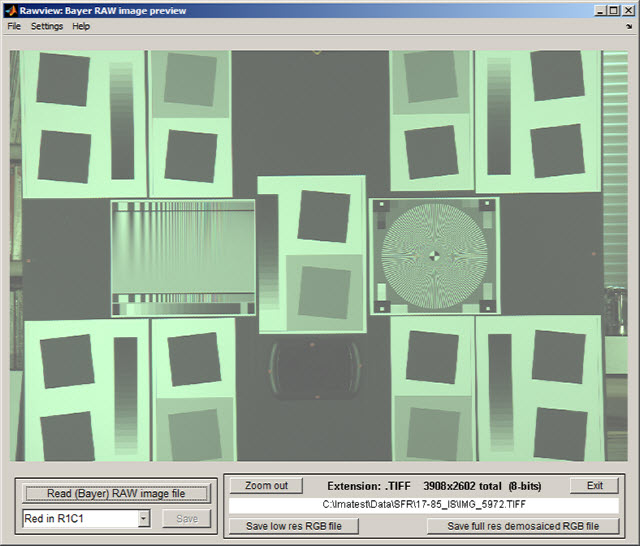
The Rawview window (no zoom)
The zoom function is always active: the image can be zoomed in to better view key details, like the red dots on the mirror, illustrated on the right, which only appear to be red when Red in R1C1 is selected. The Save button is enabled whenever the Red in RmCn selection is changed. It sets the default for opening Bayer RAW files in Imatest modules, affecting some displays.
Note that Rawview performs no White Balance, so the balance you see represents the color balance in the sensor, which may be of interest. It is rarely neutral. |
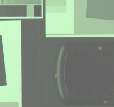
Rawview detail |
Rawview dropeown menus include display options and Save commands.
File
- Read Bayer RAW file Read the Bayer RAW file (must be in a standard image file format: TIFF, etc.)
- Save Screen Save the contents of the screen. Optionally display it if the Display screen checkbox is checked. You need to set the viewer before the first time you display the screen this way. Irfanview is an excellent free viewer.
- Save image as RGB file Save the image as an RGB file, which has half the pixel dimensions (resolution) on the original file. This does not involve a demosiacing algorithm. The contents of the R, selected G (G(R) or G(B)), and B channels are identical to the undemosaiced channels.
Settings
- Display G(R) as green Use the G(R) channel— the green pixels in the the same row as the red (R) pixels— for the green channel in the display and the RGB file save. You can tell if there is a difference between the two green channels (G(R) and G(B)) by toggling between these.
- Display G(B) as green Use the G(B) channel— the green pixels in the the same row as the blue (B) pixels— for the green channel in the display and the RGB file save.
- Adjust 16-bit images Brighten 16-bit images (which are linear or nearly so, i.e. gamma near 1.0) if needed to enhance display.
- Brighten 16-bit images Brighten 16-bit images further for additional display enhancement.
Help
- Online Help opens this page in your default web browser.
Using SFR Part 1
Setting up and photographing SFR targets
The
slanted-edge test image
Imatest SFR
measures the
spatial frequency response, also known as the Modulation
Transfer Function (MTF), of digital cameras and digitized film
images.
ISO 12233 test chart
with Imatest SFR cropping
indicated by the red rectangle.
It uses a simple slanted-edge (black-to-white) target described in Sharpness:
What is it and how is it measured? Although it doesn't provide the as strong a visual indication of MTF as the Log Frequency test chart, it provides a more accurate quantitative measurement.
Imatest SFR also measures Chromatic aberration, noise and Shannon
information capacity— a useful but unfamiliar indicator of image
quality.
Imatest SFR uses a standardized sharpening algorithm to compensate for the different amounts of sharpening in different cameras, allowing them to be fairly compared.
These instructions also apply to the Slanted-edge SFR module of Rescharts, which is performs identical calculations to Imatest SFR, but has a more interactive interface.
| Origins of Imatest SFR The algorithms for calculating MTF/SFR were adapted from a Matlab program, sfrmat, written by Peter Burns () to implement the ISO 12233 standard. Imatest SFR incorporates numerous improvements, including improved edge detection, better handling of lens distortion, and far more detailed output. A description can be found here. The original Matlab code is available on the I3A ISO tools download page by clicking on ISO 12233 Slant Edge Analysis Tool sfrmat 2.0. In comparing sfrmat 2.0 results with Imatest, keep the following in mind: If an OECF (tonal response curve) file is not entered into sfrmat, it assumes that there is no tonal response curve, i.e., gamma = 1. In Imatest, the default gamma is 0.5, which is typical of digital cameras. To obtain good agreement with sfrmat, you must set gamma to 1. |
A horizontal slanted-edge for measuring vertical MTF
performance is
shown below; a vertical slanted-edge for measuring horizontal MTF
performance
is shown on the right. These edges were cropped from an image of the
PIMA/ISO
12233 test chart taken by the Canon EOS-10D digital SLR, shown above. A crop area is indicated by a red rectangle.
|
|
Imatest Master can analyze edges of nearly any angle. For best results, exact vertical, horizontal, and 45° edges should be avoided.
|
 |
Printing,
assembling, and photographing the target
You can run Imatest SFR with any clean, sharp, straight black-to-white or dark
gray-to-white
edge. The solid areas need to be smooth and uniform: white on one side
and black or dark gray on the other. Since Imatest
does not yet sell a printed chart, the quickest way to
obtain
a chart is to print one on a high quality inkjet
printer.
Obtain a test chart.
Several alternatives are available for obtaining test charts.
- Download one of the test images below and print it on a high quality inkjet printer (details below) or send it to a lab for printing, for example, one of the labs listed by Dry Creek Photo.
- Create and print a test image with the Imatest Test Charts module. A variety of contrast ratios and highlight colors are available. Several Structured vector graphics (SVG) charts are available in Imatest Master. Some of the slanted square on an m x n grid patterns (example on right) are exceptionally well suited for printing large and for automated testing, and have numerous advantages over the ISO 12233 chart.
- Purchase a chart such as the ISO 12233 (QA-72) or QA-77 (available from Applied Image) or as a less expensive alternative from Danes-Picta in the Czech Republic (the DCR3 chart on their Digital Imaging page). The Applied Image charts are printed with much higher resolution than an inkjet printer can achieve, hence they can be use at much closer distances. Their disadvantage is that they have very high contrasts (>=40:1), which often results in reduced accuracy, and they have a great deal of wasted real estate: usable edges may not be found in regions of greatest interest such as the four corners.
- A printable vector-graphics version of the ISO 12233 chart is available courtesy of Stephen H. Westin of the Cornell University Computer Graphics Department. It should be printed as large as possible (17x22 inches (A2) minimum; 24x26 inches (A1) if possible for 8+ megapixel cameras) so measured sharpness is limited by the camera and lens, not the printer. Because of the limitations of the ISO chart (described above), the Imatest SVG charts are generally preferable.
You
can download printable test charts by right-clicking on the
thumbnails
below. The bitmap chart, which is included in the samples folder of the Imatest
installation, has pixel levels 47 and
255,
has a contrast ratio of (255/47)2.2 = 41 when printed
at gamma = 2.2 (the normal setting). This is close to the minimum
recommended
by the ISO 12233 standard (but, as we've learned recently, higher than optimum). The two SVG charts have contrast ratios of 20 and 2. Instructions for their use can be found in Test Charts. The recommended print size is letter or A4, but these charts print at maximum quality for any size.
| SVG charts — can be viewed, edited, and printed from Inkscape. Right-click on the links to save the file. Download size: 304 KB (SVG); 500 KB (PDF). |
|
Contrast = 20, light, gamma = 2.2, white highlights (SVG) | Contrast = 20 (PDF) High enough contrast to excite maximum sharpening in most cameras but low enough to avoid clipping in most cases. |
 |
Contrast = 2, middle, gamma = 2.2, white highlights (SVG) | Contrast = 2 (PDF) Relatively low contrast: little, if any, sharpening would be expected. The two charts should have the same MTF if no nonlinear processing is applied, for example, with RAW files with dcraw conversion. |
| Bitmap chart |
|
|
Edge_chart_low.png
(reduced
contrast;
pixel levels 47, 255)
|
Test images with a varety of contrast ratios and highlight colors can be created with the Imatest Test Charts module.
Nonlinear signal processing and chart contrast
Although Imatest SFR is relatively insensitive to chart contrast (MTF is normalized to 100% at low spatial frequencies), measured SFR is often affected by chart contrast due to nonlinear signal processing in cameras, i.e., processing that depends on the contents of neighboring pixels, and hence may vary throughout an image. Nonlinear processing is almost universal in digital cameras (though you can avoid it by using RAW images with dcraw). It improves pictorial quality but complicates measurements. It takes two primary forms.
- Sharpening, applied in the proximity of contrasty features like edges. Boosts response at high spatial frequencies.
- Noise reduction, applied in the absence of contrasty features. Attenuates response at high spatial frequencies, i.e., removes fine, low contrast detail (texture), which is interpreted as noise. Many cameras increase noise reduction at high ISO speeds.
The signal processing algorithms are proprietary; they are a part of a manufacturer's "secret sauce"
for producing pleasing images. Though they vary a great deal, some generalizations can be made.
Most cameras do NOT apply noise reduction and sharpening uniformly throughout an image.
Contrasty edges tend to have better (more extended) MTF than low contrast edges.
For this reason it may be a good idea to photograph both a relatively contrasty edge (though not so high that it causes clipping) as well as a relatively low contrast edge. The SVG charts (above) are excellent choices. Both types of edge can also be produced using Imatest Test Charts. An estimate of chart contrast derived from the average light and dark pixel levels (away from the transition) and gamma is displayed in several places in SFR and Rescharts Slanted-edge SFR. (Estimated chart contrast = (avg. pixel level of light area/avg. pixel level of dark area)^(1/gamma) ).
Nonlinearities are analyzed in depth in the Log F-Contrast module. |
Print the charts
The use of guide marks for tilting the chart
Print the test image with a high quality inkjet
photo printer on glossy, semigloss, or luster paper. Alternatively, send it to a lab to be printed. Dry Creek Photo has an excellent listing. I recommend
printing
at least two copies: one for measuring center sharpness and one for
edge
sharpness. Bitmap images should be printed 8x10
inches (20.3x25.4 cm) or smaller—
size is not critical. Be sure the edges look clean and sharp to
your
eyes; examine them with a good magnifier or loupe. Chart quality is
described
in detail in Chart quality and distance,
below.
The bitmap charts are intended to be tilted approximately 5.7 degrees
(anywhere
between 2 and 7 degrees is OK) when they are photographed. They are tilted
5.7 degrees when the tick marks, located near the edges, are vertically
or horizontally aligned with the center. This is illustrated by the red
horizontal and vertical lines on the right. Imatest Master can analyze edges of nearly any angle; exact horizontal, vertical, and 45° edges should be avoided for best results.
The SVG charts do not need to be tilted.
Alternatively, print it at one of the labs listed by Dry Creek Photo. The charts are printed straight and physically tilted because the
edges
print sharper that way. If they were printed at an angle, the printer
dot
pattern could cause some jaggedness. A 5.71° angle (tan-1(0.1))
is an offset of one part in 10.
Assemble the charts into a target
to be photographed.
The following target is described in detail in The Imatest Test Lab. It can be used to measure lens performance near the center, part-way out, and near all four corners. The Log F-Contrast and Star charts to the left and right of center are not necessary for lens testing; they provide information about signal processing. Slanted-edges or other charts (the Kodak Q-14 step chart or the Gretag Macbeth ColorChecker) may be substituted if your primary interest is lens testing.
Sharpness target (30x40 inch) for cameras up to 13 megapixels
The printed charts are mounted on a 32x40 inch sheet of 1/2 inch thick black foam board with spray adhesive or double-sided tape. If a ColorChecker is substituted, Velcro is recommended so it can be removed for dark storage. 1/2 inch foam board stays flatter than standard 1/4 or 3/8 inch board. Black board results in less flare light than white board. (Flare light is light that bounces between lens elements and off the inside of the lens barrel, reducing image contrast).
An image of a horizontal or vertical edge on an LCD monitor (desktop or laptop) can also be used as a target. The camera should be tilted with respect to the monitor. The image dark gray and white rather than black and white to minimize clipping. This page contains a description and an image, as well as a description of the Screen Patterns module, which can be used to create an image. The disadvantage of this technique is that you have only one edge to work with; you can't easily create a map of lens performance.
An image
of a horizontal or vertical edge on an LCD monitor (desktop or
laptop)
can also be used as a target. The camera should be tilted with
respect
to the monitor. (Thanks to Scott
Kirkpatrick for the suggestion.) The disadvantage of this technique is that you have only one edge to work with; you can't easily create a map of lens performance.
 |
To minimize artifacts (Moire, etc.) the camera must be
far enough from
the monitor so the sensor pixel "frequency" (1/(2*pixel
spacing) at the image sensor) is at least 30% above the Nyquist
frequency
of the LCD screen. A good rule of thumb is that the LCD screen image
should
take up no more than 1/3 to 1/4 the image width (1/9 to 1/16 the area),
as shown on the right.
My inexpensive Toshiba laptop, shown on the right,
displays 1024 pixels
horizontally. The Canon EOS-10D has 3072 horizontal pixels. In this
case,
the laptop image should take up no more than 1/4 the image width. |
Click here to view a web page
with a suitable
LCD test image (dark gray and white rather than black and white to
minimize clipping).
|
Photograph the target.
|
Frame the chart so there are usable edges near the center, part-way out, and near the corners. Take care that the chart is properly aligned. A number of useful alignment techniques and tricks are presented in The Imatest Test Lab.
|
|
Lighting
The chart below summarizes lighting considerations. The goal is even, glare-free illumination. Lighting angles between 30 and 45 degrees are ideal in most cases. At least two lights (one on each side) is recommended; four or six is better. Avoid lighting behind the camera, which can cause glare. Check for glare and lighting uniformity before you expose. A detailed description of the recommended lighting setup, which uses six high quality (CRI > 98) 4700K (near-daylight) 50W SoLux quartz-halogen lamps, can be found in The Imatest Test Lab. SoLux Task Lamps may also be used. The BK Precision 615 Light meter (Lux meter) is an outstanding low-cost instrument (about $100 USD) for measuring the intensity and uniformity of illumination.
Distance
| Distance and field of view |
| The camera must be far enough from the chart so you are measuring the sharpness of your camera and lens, not the chart. But remember, |
It's the field of view, not the chart-to-camera distance, that counts.
|
| A rough rule of thumb: For an inkjet-printed chart the field of view should be at least |
22 inches (60 cm) for a 6-megapixel camera;
35 inches (90 cm) for a 16 megapixel camera. |
| Details below. For a high-quality photographically-printed chart (such as the charts from Applied Imaging) you can get quite a bit closer. |
|
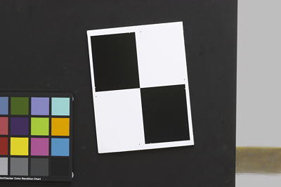 A letter-sized (8.5x11 inch) chart printed on Permium Luster paper on the Epson 2200 (a high quality pigment-based inkjet photo printer) was analyzed for MTF using the 6.3 megapixel Canon EOS-10D. There was no change when the image field was at least 22 inches (56 cm) wide— twice the length of the chart. Performance fell off slowly for smaller fields.
Choose a camera-to-target distance that gives at least this image field width. The actual distance depends on the sensor size and the focal length of the lens. The minimum image field is illustrated on the right.
Commercial charts are often printed at higher resolutions than inkjet printers can achieve, and hence may be used at shorter distances— microscopic in some cases. For example, the small Applied Image/Sine Patterns ISO-12233 Resolution Charts (.1X, .5X, and 1X) are printed on photographic paper, which is capable of extremely fine resolution. The chart may safely fill the entire frame.
Cameras with more pixels, and hence higher potential resolution,
should
should have a larger image field width.
Distance/field width guidelines for high quality inkjet charts
(You can get closer with photographically-printed charts.) |
| The
camera-to-target
distance is not critical as long as it is greater than a reasonable
minimum. |
Sensor sizes |
Desig-
nation |
Diagonal
mm. |
Width
mm. |
Height
mm. |
| 1/3.6" |
5.0 |
4.0 |
3.0 |
| 1/3.2" |
5.68 |
4.54 |
3.42 |
| 1/3" |
6.0 |
4.8 |
3.6 |
| 1/2.7" |
6.59 |
5.27 |
3.96 |
| 1/2" |
8.0 |
6.4 |
4.8 |
| 1/1.8" |
8.93 |
7.18 |
5.32 |
| 2/3" |
11.0 |
8.8 |
6.6 |
| 1" |
16.0 |
12.8 |
9.6 |
| 4/3" |
22.5 |
18.0 |
13.5 |
| 35mm |
44.3 |
24.0 |
36.0 |
|
Image field
width (in inches) > 8.8 × sqrt(megapixels)
( > means "greater than.")
Image field
width (in
cm) > 22 × sqrt(megapixels)
— or —
There should
be no more
than 140 sensor pixels per inch of target or 55 sensor pixels per
centimeter
of the target.
— or —
The distance
to the target
should be at least 40X the focal length of the lens for 6-10 megapixel digital SLRs.
(25X
is the absolute minimun for 6 megapixel DSLRs; 40X leaves some margin.) For compact digital
cameras,
which have much smaller sensors, the distance should be at least 100X
the actual
focal length: the field of view is about the same as an SLR with
comparable
pixel count. The recommended distance is described in more detail in Chart
quality and distance, below. |
There is some confusion about lens focal lengths in compact digital cameras. They are often given as the "35mm-equivalent," which many photographers can relate to viewing angle. 35-105mm or 28-140mm are typical "35mm-equivalent" numbers, but they are not the true lens focal length, which is often omitted from the specs. What is given is the sensor size in 1/n inches, a confusing designation based on the outside diameter of long-obsolete vidicon tubes. It The table on the right relates the 1/n designation to the diagonal dimension of the sensor.
True focal length = "35mm-equivalent" × (diagonal mm.) / 44.3 |
Exposure
|
|
Proper exposure is important
for accurate Imatest SFR
results.
Neither the black nor the white regions of the chart should clip—
have substantial areas that reach pixel levels 0 or 255. The best way
to
ensure proper exposure is to use the histogram in your digital camera.
Blacks (the peaks on the left) should be above the minimum and whites
(the
peak(s) on the right) should be below the maximum.
|
|
Low contrast test charts (with contrast ratios of 40:1 or lower) are helpful for avoiding clipping.
The above image (taken from the Canon File Viewer Utility) is close
to a perfect exposure.
| Tips
on photographing the chart |
| Distance
doesn't matter
as long as the target far enough from the camera so sharpness is
limited
by the camera and lens, not
by the target. For a target printed on the Epson 2200 printer, a
distance
that gives at least a 24 inch (horizontal) field of view seems to be
sufficient. |
| The target
should be evenly
lit and free of glare. |
| White
balance should be
approximately neutral. |
| Use a
sturdy tripod and
a cable release. If possible, use the mirror lock. You can use Imatest
SFR to find the difference made by a good tripod or mirror lock— to
sharpen
your technique, literally ( pun intended ). |
| Be sure to
expose the image
so detail is maintained in both light and dark areas. Neither should be
blocked (clipped). Use your camera's histogram. If more than 0.5% of
the
pixels are at levels 0 or 255, Imatest SFR will assume that clipping
has
taken place and issue a warning message. This has no effect on the
calculations—
it's just a warning that accuracy may be compromised. |
| Be sure
the camera is correctly
focused on the chart. |
| Place
slanted-edge images
near the corners of the field as well as near the center. |
| You may
find it instructive
to photograph the slanted edge target along with a target from Lens
testing, but there's no need to do so. |
|
Save the image as a RAW file or maximum quality JPEG. If you are
using
a RAW converter, convert to JPEG (maximum quality), TIFF (without LZW
compression,
which is not supported), or PNG. If you are using film, develop and
scan
it. The file name should be descriptive and should indicate the
parameters
you are testing. Use dashes and underscores ( - and _ ), but avoid
spaces.
(Spaces work with Imatest, but they can be troublesome in DOS command
lines
and web pages.) An example would be Canon_EOS10D_70-200f4L_100mm_f8_ctr.jpg.
You are now ready to run
Imatest
SFR.
| Chart
quality and distance |
Three printed charts were scanned with the Epson 3200
flatbed scanner
at 1200 dpi— a much higher scan density than normal for reflective
documents
(300 or 400 dpi). At a typical monitor resolution of 96 dpi, the images
are enlarged 12.5x. The charts were tilted around 5.7 degrees (a 1.1
inch offset on an
11 inch letter-sized print) for analysis with Imatest SFR.
Epson 2200
Premium Glossy 1440 dpi
High contrast
|
Epson 2200
Premium Glossy
1440 dpi
Reduced contrast
|
HP LaserJet 5L
bond paper
Reduced contrast
|
The high contrast chart appears to be the
sharpest. The reduced contrast
chart is still very good: its dot pattern (always a concern) is not a
problem.
The laser print is clearly unsuitable.
Results of running Imatest
SFR on the high contrast printed chart are shown below. The SFR input
dialog
box was set to display cycles/millimeter for 1200 pixels/inch (scan
density).
The key result is MTF50 (50% contrast spatial frequency) = 5.15
cycles/millimeter
(131 cycles/inch). Results in LW/PH and with standardized sharpening
(indicated
by (corr.); dashed red lines) are not
applicable.
As expected, the reduced contrast chart, which
doesn't appear as sharp,
has a lower MTF50: 4.31 cycles/mm (109 cycles/inch). It would benefit
from
sharpening in the image editor.
The chart MTF50 affects the minimum recommended
camera-to-target distance.
For example, the Canon EOS-10D (and 300D) has a pixel spacing of 7.4
microns.
Its Nyquist frequency is 1000/(2*7.4) = 68
cycles/mm.
When the target is 40x the lens
focal
length, so the magnification at the sensor is approximately 1/40
(recommended
above), the MTF50 imaged on the sensor for the reduced contrast chart
is
4.31*40 = 172 cycles/mm, which is 2.5 times the Nyquist frequency. The
imaged target contrast is approximately 0.9 in the critical region
around
0.6*Nyquist (0.3 cycles/pixel). This is adequate, though a little more
distance) (e.g., 50x focal length)
wouldn't hurt. |
|
A print of Stephen H. Westin's printable vector-graphics version of the ISO 12233chart, made on the Epson 2200 at 1440 dpi on Premium Luster paper and scanned by the Epson 3200 at 1200 dpi, has been analyzed to compare slanted and straight edges. The comparison is of interest because Stephen's chart uses vector graphics, hence the slanted edge is as fine as the printer can make; it is not limited by image pixels. Straight and slanted edges where compared with the print scanned straight and tilted.
The straight edge is clearly smoother than the slanted edge, though the sharpness of the individual edges (horizontal scan lines) is about the same. This MTF results are surprizing: MTF50 for the slanted edge scanned straight is 4.13 cycles/mm, not very different from MTF50 for the straight edge scanned tilted, 4.24 cycles/mm. The difference is more pronounced at lower MTFs (higher spatial frequencies). MTF20 for the slanted edge scanned straight is 8.6 cycles/mm while MTF20 for the straight edge scanned tilted is 10.6 cycles/mm. I clearly perfer the straight edge, tilted. Although the numbers suggest it would make little difference, I recommend a 20% greater distance if the slanted edge is used.
The results in this box are for charts printed on high quality inkjet printers. Commercially-available charts are often printed at higher resolution, and hence may be used at shorter distances— microscopic in some cases. |
|
Using SFR Part 2
Running Imatest SFR
Running
Imatest SFR
Imatest is opened by double-clicking the Imatest icon on
- the Desktop,
- the Windows Start menu,
- the Imatest folder (typically C:\Program files\Imatest in English language installations).
After several seconds, the Imatest main window, shown below, opens. Then click on SFR: New file or Rescharts on the upper left. The SFR: Current file button is grayed out (inoperative) for the first run because no file has yet been read. It can be used in succeeding runs to save time when analyzing different regions, though multiple ROI (region of interest) runs are more efficient. (The input image is cleared to save memory and SFR: Current file is grayed out if another module is run.)
The Imatest main window
Several cropped slanted-edge JPEG images are included in the images
subfolder of the Imatest folder. Complete ISO12233 chart images are not
included with Imatest because they are large (usually over 2 megabytes).
They can be downloaded from dpreview.com reviews, typically in the last page titled "Compared to...," and from Imaging-resource.com reviews, typically on the page labeled "sample images."
Selecting
the image file (or batches of files)
When you click SFR: New file from the Imatest main window or Read image file (with Slanted-edge SFR selected) from Rescharts, the window below appears, requesting the image file name(s). The folder saved from the previous run appears in the Look in: box on the top. You are free to change it. You can open a single file by simply double-clicking on it. You can select multiple files (for batch mode or combined runs with SFR in Imatest Master) by the usual Windows techniques: control-click to add a file; shift-click to select a block of files. Then click Open. Three image files for the Canon 17-40mm L lens (taken with the EOS-10D) are highlighted. Large files can take several seconds to load. Imatest remembers the last folder used (for each module, individually). In batch mode the first file is handled like a normal run; the remaining files run in express mode (no dialog boxes).
File selection
If the folder contains meaningless camera-generated file names such as IMG_3734.jpg, IMG_3735.jpg, etc., you can change them to meaningful names that include focal length, aperture, etc., with the View/Rename Files utility, which takes advantage of EXIF data stored in each file.
| Multiple file selection Several files can be selected in Imatest Master using standard Windows techniques (shift-click or control-click). Depending on your response to the multi-image dialog box you can combine (average) several files or run them sequentially (batch mode). |
Combined (averaged) files are useful for measuring the effects of image stabilization. The combined file can be saved. Its name will be the same as the first selected file with _comb_n appended, where n is the number of files combined. |
Batch mode allows several files to be analyzed in sequence. There are three requirements. The files should (1) be in the same folder, (2) have the same pixel size, and (3) be framed identically. |
The input dialog box for the first run is the same as for standard non-batch runs. Additional runs use the same settings. Since no user input is required they can run extremely fast. |
If the order of the files in a batch runs is different from the selection order, click Settings, Options and Settings... (in the Imatest main window) and change the setting in Batch run order. The sequence may be affected by Windows Explorer settings. |
One caution: Imatest can slow dramatically on most computers when more than about twenty figures are open. For this reason we recommend checking the Close figures after save checkbox, and saving the results. This allows a large number of image files to be run in batch mode without danger of bogging down the computer. |
|
| RAW files Starting with Imatest Master 2.7 (February 2008) Imatest SFR can analyze Bayer raw files: standard files (TIFF, etc.) that contain undemosaiced data. RAW files are not very useful for measurring MTF because the pixel spacing in each image planes is twice that of the image as a whole; hence MTF is lower than for demosaiced files. But Chromatic aberration can be severely distorted by demosaicing, and is best measured in Bayer RAW files (and corrected during RAW conversion). Details of RAW files can be found here. |
Selecting
the ROI (Region of Interest)
If the image has the same pixel dimensions as the image in the previous run, a dialog box shown below asks you if you want to repeat the same ROIs (regions of interest) as the previous image. You can retrieve saved ROIs from past runs by clicking on Retrieve settings in the Imatest main window.
|
If you answer No or if the image has a different size, the coarse selection dialog box shown on the right is displayed with the instructions, Select
ROI by clicking and dragging, or clicking outside image.
Click on one corner of the intended region, drag the
mouse to the other corner, then release the mouse button. Click outside
the image to select the entire image.
Note: the Zoom feature of Matlab Figures does not work here. Imatest mistakenly assumes you are trying to select the entire image. To enlarge the image (to view the crop area more clearly), maximize it by clicking on the square next to the upper right corner of the Window. |
ROI selection: ISO 12233 chart
|
After you make your selection the ROI find adjustment dialog box, shown below, appears. You can move the entire ROI or any of the edges in increments of one pixel. You can also enter the ROI boundary locations in the boxes below the image. If you do this, be sure to press return (or move the cursor) to register the change. You can zoom out to view the entire image, then zoom back in. The ROI fine adjustment is particularly valuable for maximizing the size of small regions and excluding interfering detail.
ROI fine adjustment
When you finish adjusting the ROI, proceed by selecting one of five choices at the bottom of the box.
| Yes, Continue |
The selected ROI is correct;
no more ROIs are to be selected. Continue with SFR calculations in normal
mode: You will be asked for additional input data, etc. |
| Yes, Continue in Express mode |
The selected ROI is correct;
no more ROIs are to be selected. Continue with SFR calculations in Express
mode: You will not be asked for additional input data or for Save options.
Saved or default settings will be used. |
| Yes, select another region |
The selected ROI is correct.
Select another ROI. For multiple ROIs additional Figures will display performance
as a function of distance from the image center. |
| No, try again |
The selected ROI is not
correct. Try again. |
| Cancel |
Cancel the SFR run. Return
to the Imatest main window. |
|
If the the height or width of the ROI is under 10 pixels, the ROI is over 250,000 pixels or appears to be inappropriate, you'll be asked to repeat the selection. The ROI is normally checked for validity, but there are some cases (e.g., endoscopes) where valid images may fail the usual tests ROI filtering can be relaxed considerably by opening the Options and Settings... button in the Imatest main window (Pro only) and clicking Light filtering in the first group of controls. This can can lead to errors when regions are selected carelessly. Normal filtering is the default.
After the run is complete, you can save ROIs for future runs in a named file by clicking on Save settings in the Imatest main window. These settings can be retrieved later by clicking on Retrieve settings.
Cropping recommendations
For best accuracy the length should be between 80 and 500 pixels. Little is gained for lengths over 300 pixels. The absolute minimum and maximum crop dimensions are 10 and 1200 pixels (800 for strong filtering).
If possible, the width (height in the image on the right) should be at least 50 pixels. Minimum widths for light and dark zones should be at least 10 pixels, with 20 preferred. Little is gained for minimum dark/light zone widths over 40 pixels or total width over 100 pixels. |
|
My typical crops are between around 120x80 and 300x140 pixels.
For very small crops (width or length between 10 and about 25 pixels) a warning message may appear in place of the light/dark level display: Zero counts in n bins. Accuracy may be reduced. This indicates that some interpolation was required to obtain the final results, which may not be as accurate or repeatable as they would be for larger ROIs.
Small crops or noisy images may require weaker error filtering than normal crops/images. Press Options & Settings... in the Imatest main window and set SFR ROI filtering to Light filtering.
Saving ROIs between runs. ROIs may be saved in named files by clicking on the Save settings button on the right of the Imatest main window. To restore the old settings, click on the Retrieve settings button. This allows you to recover old ROIs after runs with different image sizes and ROIs.
SFR input dialog box
The Imatest SFR input dialog window, shown below, opens after the Region of
Interest (ROI) has been selected, except when Express mode has been selected.
It appears only once during multiple ROI runs. Succeeding runs use the
same settings except for (calculated) Crop location.
All input fields are optional. Most of the time you can simply click OK (the button on the lower right) to continue.
SFR input dialog box
This window is divided into sections: Title and Help on top, then Plot, Options, Settings, Optional parameters, and finally, OK or Cancel.
Title
defaults
to the input file name. You may leave it unchanged, replace
it, or add descriptive information for the camera, lens, converter settings, etc.— as
you please.
Help opens a browser window containing a web page describing the module. The browser window sometimes opens behind other windows; you may need to check if it doesn't pop right up.
Plot
selects figures to plot. These figures are listed on the left. Plot settings are saved.
Only Cycles per (pixel) and Chromatic Aberration are checked by default. The LW/PH (or LP/PH) plot
is unchecked (by default) because it is largely redundant.
The boxes to the right of "Cycles
per" control the x-axis display. You can choose between
Cycles
per pixel (the default), Cycles
per inch, or
Cycles
per mm. If you choose Cycles
per inch or mm,
you must enter a number for the pixel size— either in pixels
per inch,
pixels
per mm, or microns
per pixel. If pixel size is omitted, the x-axis will be displayed in Cycles
per pixel. For the second plot you can choose between LW/PH and LP/PH (Line Pairs per Picture Height).
Pixel size has an important relationship to image quality. For very small pixels, noise, dynamic range and low light performance suffer. Pixel size is rarely given in spec sheets: it usually takes some math to find it. If the sensor type and the number of horizontal and vertical pixels (H and V) are available, you can find pixel size from the table on the right and the following equations.
pixel size in mm = (diagonal in mm) / sqrt(H2 + V2)
pixel size in microns = 1000 (diagonal in mm) / sqrt(H2 + V2)
Pixel size in microns (microns per pixel) can be entered directly into the SFR input dialog box. Example, the cute little 5 megapixel Panasonic Lumix DMC-TZ1 has a 1/2.5 inch sensor and a maximum resolution of 2560x1980 pixels. Guessing that the diagonal is 7 mm, pixel size is 2.1875 (rounded, 2.2) microns.You can find detailed sensor specifications in pages from Sony, Panasonic, and Kodak. |
Sensor
Designation
(Type) |
Diagonal
mm. |
Width
mm. |
Height
mm. |
| 1/4" |
4.5 |
|
|
| 1/3.6" |
5.0 |
4.0 |
3.0 |
| 1/3.2" |
5.68 |
4.54 |
3.42 |
| 1/3" |
6.0 |
4.8 |
3.6 |
| 1/2.7" |
6.59 |
5.27 |
3.96 |
| 1/2.5" |
6.9 - 7.2 |
|
|
| 1/2" |
8.0 |
6.4 |
4.8 |
| 1/1.8" |
8.93 - 9.1 |
7.18 |
5.32 |
| 2/3" |
11.0 |
8.8 |
6.6 |
| 1" |
16.0 |
12.8 |
9.6 |
| 4/3" |
22.5 |
18.0 |
13.5 |
| 35mm |
44.3 |
24.0 |
36.0 |
|
For the Multi-ROI plot you can choose between Off, 1D plots (results as a function of center-corner distance with MTF in Cycles/Pxl, LW/PH), 2D image plots (results superimposed on image with MTF in Cycles/Pxl, LW/PH). You can also plot multi-ROI SQF (Subjective Quality Factor), which is explained here.
Noise spectrum and Shannon capacity is unchecked by default because the results are difficult for most users
to interpret and may not be meaningful, especially when significant noise reduction has been applied. It will not be plotted if the selected region is too small for adequate noise statistics. If both Chromatic Aberration and Noise spectrum and Shannon capacity are checked, the two plots share the same figure: CA on top and Noise/Shannon capacity at the bottom.
Display options (to the right of Plot) are settings that affect the plot display.
 Secondary readout controls the secondary readout display in MTF plots. The primary readout is MTF50 (the half-contrast spatial frequency); the secondary readout has several options. It defaults to MTF30 (the spatial frequency where MTF is 30%).
Clicking Change opens the window shown on the right. Secondary readout settings are saved between runs. Choices:
- The upper radio button (MTF) selects MTFnn, the spatial frequency where MTF is nn% of its low frequency value.
- The middle radio button selects MTFnnP, the spatial frequency where MTF is nn% of its peak value: useful with strongly oversharpened edges.
- The lower radio button (MTF @ ) selects MTF @ nn units, where nn is a spatial frequency in units of Cycles/pixel, LP/mm, or LP/in. If you select this button, the pixel spacing should be specified in the Cycles per... line in the Plot section of the input dialog box, shown above. A reminder message is displayed if the pixel spacing has been omitted.
MTF plot freq selects the maximum display frequency for MTF plots. The default is 2x Nyquist (1 cycle/pixel). This works well for high quality digital cameras, not for imaging systems where the edge is spread over several pixels. In such cases, a lower maximum frequency produces a more readable plot. 1x Nyquist (0.5 cycle/pixel), 0.5x Nyquist (0.25 cycle/pixel), and 0.2x Nyquist (0.1 cycle/pixel) are available.
Edge plot selects the contents of the upper (edge) plot. The edge can be cropped (default) or the entire edge can be displayed. Three displays are available.
- Edge profile (linear) is the edge profile with gamma-encoding removed. The values in this plot are proportional to light intensity. This is the default display.
- Line spread function (LSF) is the derivative of the linear edge profile. MTF is the fast fourier transform (FFT) of the LSF. When LSF is selected, LSF variance (σ2), which is proportional to the DxO blur unit, is displayed.
- Edge pixel profile is proportional to the edge profile in pixels, which includes the effects of gamma encoding.
Chart contrast For a medium or low contrast charts (contrast <= 40; not recommended with the old ISO 12233 chart), you can enter the chart contrast (or Off). If the ROI is large enough, the actual (measured) gamma will be calculated and displayed along with the contrast factor (the chart contrast multiplier = measured gamma/nominal gamma, where nominal gamma is entered in the Settings area, described below). If the Use for MTF box just to the right is checked, this value will be used in the MTF calculation, which may result in a modest improvement in accuracy.
Reset restores the settings in Options and Settings to their default values.
Settings affect the calculations as well as the display.
Gamma is
used to linearize the input data, i.e., to remove the gamma encoding applied in the camera or RAW converter. It defaults to 0.5
= 1/2, which is typical of digital cameras, but is affected by camera or RAW converter contrast settings. It may
be quite different for scanned film images. It should be set to 0.45 when RAW images are read into Imatest (to be converted by dcraw), but there is little loss in accuracy if you leave it at 0.5. If is is set to less than 0.3 or greater than 0.8, the background will be changed to pink to indicate an unusual (possibly erroneous) selection.
Since SFR sharpness measurements are moderately sensitive to the
Gamma setting (a 10% error in gamma results in a 2.5% error in MTF50 for a normal contrast target), it's a good idea to run Colorcheck or Stepchart to determine the correct value of Gamma. A nominal value of gamma should be entered, even if the value of gamma derived from the chart (described above) is used to calculate MTF.
| Gamma |
Gamma is the exponent of the equation that relates image pixel level to luminance. For a monitor or print,
Output luminance = (pixel level)gamma_display
When the raw output of the image sensor, which is linear, is converted to image file pixels for a standard color space, the approximate inverse of the above operation is applied.
pixel level = (RAW pixel level)gamma_camera ~= exposuregamma_camera
The total system gamma is gamma_display * gamma_camera. Standard values of display gamma are 1.8 for older color spaces used in the Macintosh and 2.2 for color spaces used in Windows, such as sRGB (the default) and Adobe RGB (1998). |
In
characteristic curves for film and paper, which use logarithmic scales (e.g.,
density (–log10(absorbed light) vs. log10(exposure)),
gamma is the average slope of the transfer curve (excluding the "toe" and "shoulder"
regions near the ends of the curve), i.e.,
Gamma is contrast.
See Kodak's
definition in Sensitometric
and Image-Structure Data.
To obtain the correct MTF, Imatest must linearize the pixel levels— the camera's gamma encoding must be removed.
That is the purpose of Gamma in the SFR input dialog box, which defaults to 0.5,
typical for digital cameras. It can, however, vary
considerably with camera and RAW converter settings, most notably
contrast.
Characteristic curves for the Canon EOS-10D with three RAW converter
settings are shown on the right. Gamma deviates considerably from 0.5.
Gamma = 0.679 could result in a 9% MTF50 error. For best accuracy we
recommend measuring
gamma using
Colorcheck or Stepchart, which provides slightly more detailed results.
Confusion factor: Digital
cameras rarely apply an exact gamma curve: A "tone reproduction curve" (an
"S" curve) is often superposed on the gamma curve to extend dynamic range while maintaining visual contrast.
This reduces contrast in highlights and (sometimes) deep shadows while maintaining or boosting
it in middle tones. You can see it in curves 1 and 3, on the right. For
this reason, "Linear response" (where no S-curves is applied on top of
the gamma curve) is recommended for SFR measurements.
The transfer function may also be adaptive:
camera gamma may be higher for low contrast scenes than for
contrasty scenes. This can cause headaches with SFR measurements. But
it's not a bad idea generally; it's quite similar to the development
adjustments (N-1, N, N+1, etc.) in Ansel Adams' zone
system. For this reason it's not a bad idea to place a Q-13 or Q-14 chart near the slanted edges.
To learn more about gamma, read Tonal
quality and dynamic range in digital cameras and Monitor
calibration. |
The three curves below, produced by Stepchart for the Canon EOS-10D, show how Gamma varies with RAW converter settings.
 1. Capture One LE set to Film standard (the default). Gamma = 0.679.

2. Capture One LE set to Linear response. Gamma = 0.508. Recommended for SFR runs.

3. Canon FVU set to Standard contrast. Gamma = 0.642.
|
|
Standardized sharpening If the checkbox is checked, standardized sharpening results are displayed as thick red curves and readouts in the edge and MTF plots. If it is unchecked, standardized sharpening are omitted, which reduces the visual clutter. Results for individual R, G, and B channels are displayed with more prominence (in Imatest Master), and edge noise is displayed. The MTF .CSV summary file is unaffected.
Standardized sharpening is an algorithm that allows cameras with different amounts of sharpening to be compared on a reasonable basis. It does so by increasing or decreasing the amount of sharpening to compensate for oversharpened or undersharpened images. Standardized sharpening radius controls the sharpening radius. Its default value of 2 (pixels) is a typical sharpening radius for compact digital cameras, which have tiny pixels. Smaller sharpening radii may be appropriate for digital SLRs, which have larger pixels and tend to have more conservative sharpening. (Imaging-resource.com uses R = 1 for DSLRs.) Sharpening radius varies for different RAW converters and settings. So you may occasionally want to experiment with the sharpening radius. Results with standardized sharpening should not be used for comparing different lenses on the same camera. For more detail, see What is standardized sharpening, and why is it needed for comparing cameras? Standardized sharpening should be unchecked for most applications.
If a an edge is too broad for standardized sharpening to work well at the specified radius, the radius is automatically increased unless Fixed sharpening radius in the Settings menu of the Imatest main window has been checked.
Channel is normally left at it's default value of Y for the luminance channel,
where Y = 0.3*R + 0.59*G + 0.11*B.
In rare instances the R, G, and B color channels might be of interest.
Picture Width and Height defaults
to the width and height of the input image in pixels, assuming landscape format,
where height < width. If the input image
has been cropped, or if it doesn't represent the entire camera image, Picture
Height (and Width) should be entered manually.
Line Width per Picture Height (LW/PH) or LP/PH results are correct only if the
Picture Height represents the entire uncropped frame. For example, Picture
Height should be 2048 for the Canon EOS-10D and 1944 for the Canon
G5 (the cameras in the cropped sample files), etc.
| For
film and scanner users |
| More film/scanner users
than I expected are using Imatest. And film users prefer
results in Line Pairs per mm (LP/mm). You can select cycles (line pairs)
per inch or millimeter in the Plot box. Scanned images tend to be cropped by the time they are entered into Imatest because complete images are
huge. (Try running the numbers for a 4,000 dpi scanner.) In this case, you
must manually enter the picture height in pixels to get LW/PH or LP/PH. The best way
is to use the equation, |
|
Picture height (pixels) = picture height (mm) * pixels/mm. |
| For example, a 4,000 dpi scanner has 4000/25.4
= 157.5 pixels/mm. For 35mm film, the picture height is 24 mm = 3780 pixels.
With medium format cameras, the picture height is somewhat smaller than
the nominal size. It is 41.5 mm for the 645 format and 56mm for the 6x6
and 6x7 (cm) formats. Picture Width is optional, but it's a good idea to enter it. It is calculated in the same way. |
|
Crop location
is the position of the center of the selected ROI (Region of interest),
expressed as the percentage the distance from the image center to the corner.
The orientation of the ROI with respect to the image center is included.
It is blank if the input image has not been cropped. Crop location can
be entered manually. This is only recommended when that image has been
cropped outside of Imatest SFR.
Additional parameters
(all optional) for Excel .CSV output contains a detailed description of the camera, lens, and test conditions. EXIF data
is entered, if available, but can be overridden by manual settings. Description & settings is particularly useful for annotating the test system (it is displayed in MTF Compare).These settings are optional but can be useful when several
tests are run for different lenses, focal lengths, apertures, or other
settings. The settings are displayed next to the MTF plots. They are saved and reused in subsequent runs for files with the same pixel dimensions. If EXIF data is available (currently, only in JPEG files) it overrides the saved settings. The Reset button clears all entries.
ISO standard SFR If this checkbox is checked, SFR calculations are performed according to the ISO 12233 standard, and the y-axis is labeled SFR (MTF) (ISO standard). This method is slightly less accurate than the normal Imatest calculation, which incorporates a number of refinements, including a better edge detection algorithm and a second-order polynomial fit to the average edge for a more accurate estimate of SFR in the presence of lens distortion. This box is normally left unchecked; it should only be used for comparing normal Imatest calculations to the ISO standard. The difference is typically very small.
When entries are complete, click OK.
A Calculating...
box appears to let you know that calculations are proceeding. Results appear
in individual windows called Figures (Matlab's standard method
of displaying plots). Figures can be examined, resized, maximized, and
closed at will. A zoom function is also available. Their contents are described in the pages on Imatest
SFR results: MTF (Sharpness) plot, Chromatic Aberration, Noise, and Shannon Capacity plot, and Multiple ROI (Region of Interest) plot.
Warnings
A Clipping warning is issued if more than 0.5% of the pixels are clipped (saturated), i.e., if dark pixels reach level 0 or light pixels reach the maximum level (255 for bit depth = 8). This warning is emphasized if more than 5% of the pixels are clipped. Clipping reduces the accuracy of SFR results. It makes measured sharpness better than reality. |
|
The percentage of clipped pixels is not a reliable index of the severity of clipping or of the measurement error. For example, it is possible to just barely clip a large portion of the image with little loss of accuracy. The plot on the right illustrates relatively severe clipping, indicated by the sharp "shoulder" on the black line (the edge without standardized sharpening). The sharp corner makes the MTF look better than reality. The absence of a sharp corner may indicate that there is little MTF error. |
Clipping warnings |
Clipping can usually be avoided with a correct exposure-- neither too dark nor light. A low contrast target is recommended for reducing the likelihood of clipping: it increases exposure latitude and reduces the sensitivity of the MTF results to errors in estimating gamma.
Two precautions
when working with figures
Too
many open Figures
Figures can proliferate
if you do a number of runs, especially SFR runs with multiple regions,
and
system performance suffers if too many
Figures are open. You will need to manage them. Figures
can be closed individually by clicking X on the upper right of the
Figure or by any of the usual Windows techniques. You can close them all
by clicking Close figures in the Imatest main window. For large batch runs, the Close figures after save checkbox in the SFR Save dialog box prevents a buildup of open figures. |
Clicking
on Figures during calculations
can confuse Matlab. Plots
can appear on the wrong figure (usually distorted) or disappear altogether.
Wait until all calculations are complete— until the Save or Imatest main
window appears— before clicking on any Figures. |
Saving
the results
|
At the completion of the SFR calculations the Save SFR
results? dialog box appears, except in Express mode, which uses previous settings. It allows you to choose which results to save and where
to save them. The default is subfolder
Results
of the data file folder. You can change to another existing folder,
but new results directories must first be created outside of Imatest using
a utility such as Windows Explorer. (This is a limitation of this version
of Matlab.)
Saved figures, CSV, and XML files are given names that consist of a root file name (which defaults to the image file name) with a suffix added. Examples:
Canon_17-40_24_f8_C1_1409_YR7_cpp.png
Canon_17-40_24_f8_C1_1409_YR7_MTF.csv
The root file name, Canon_17-40_24_f8_C1_1409_YR7, can be overridden by entering another name in the Results root file name: box. Be sure to press the Enter key. This feature does not work with batch runs.
Checking Close figures after save is recommended for preventing a buildup of figures (which slows down most systems) in batch runs. |
SFR save dialog box |
When multiple ROIs are selected, the Save
results? dialog box appears only after the first set
of calculations. The remaining calculations use the same Save settings. Save
results? is omitted entirely in an Express
run for repeated images.
The first four checkboxes are for the figures, which can be examined before the boxes are checked or unchecked. After you click on Yes or No, the selections are saved, then the Imatest main window reappears.
Result file
names— The roots of the file names are
the same as the image file name. The channel (Y, R, G, or B) is included
in the file name. If a Region of Interest has been selected from a complete
digital camera image, information about the location of the ROI is included
in the file name following the channel. For example, if the center of the
ROI is above-right of the image, 20% of the distance from the center to
the corner, the characters AR20 are included in the file name.
Output files
for filename.jpg (Y-channel)
(default location:
subdfolder Results)
| Figures
(.PNG image files) |
| filename_YA17_cpp.png |
Plot with x-axis in cycles/pixel (c/p), Y-channel,17% of the way to
the corner above the center of the uncropped image. |
| filename_YA17_lwph.png |
Plot with x-axis in Line Widths per Picture Height (LW/PH). |
| filename_YA17_ca.png |
Plot of Chromatic Aberration, with noise statistics and Shannon information
capacity. |
| Excel
.CSV (ASCII text files that can be opened in Excel) |
| CSV output files are explained in detail below. Click link for detail on individual file. |
| SFR_cypx.csv |
(Database file for appending results: name does not change). Displays
10-90% rise in pixels and MTF in cycles/pixel (C/P). |
| SFR_LWPH.csv |
(Database file for appending results: name does not change). Displays
10-90% rise in number/Picture Height (/PH) and MTF in Line Widths per Picture
Height (LW/PH). |
| filename_YA17_MTF.csv |
Excel .CSV file of MTF results for this run. All channels (R, G, B, and Y (luminance) ) are displayed.The first row has the
headers: cy/pxl, LW/PH, MTF(nchan), MTF(corr), MTF(R), MTF(G), MTF(B), MTF(Y), where nchan is the selected channel. The remaining lines contain the
data. Can easily be plotted or combined with data from other files. |
| filename_Y_multi.csv |
Excel .CSV file of summary results for a multiple ROI run. |
| filename_Y_sfrbatch.csv |
Excel .CSF file combining the results of batch runs (several files) with multiple ROIs. Particularly useful for generating easily-readable Excel plots. |
The PNG files are identical to the Imatest
Figures, except that the background is white instead of gray.
Average edge and MTF plot (primary results of SFR)
These results are explained in Sharpness: What is it and how is it measured?
Repeated
runs
|
If SFR was previously run with an image of the same pixel dimensions and you click on either of the Run
SFR buttons, an image that displays the selected ROIs
appears on the left of the screen and you'll be asked, "Do
you want the same ROIs as the previous image?" A portion
of the previous image and the ROI repeat box
are shown in the image on the right.
|
ROI repeat dialog box: Imatest Studio |
| Yes |
Use the previous crop. Open SFR input dialog box. |
| Yes, Express mode |
Use previous crop and run in Express mode.
Do not open the
input dialog box;
use saved data instead. Save dialog boxes are also omitted.
Some warnings are suppress. Speeds up repeated runs, e.g., testing several apertures. |
| Yes, Adjust ROI |
Open a fine adjustment dialog box (shown below), starting with the previous selection.
Useful for a sequence of runs with similar, but not identical, framing.
Imatest Studio: Only available when a single ROI is selected.
Imatest Master : For multiple ROIs, a window that allows ROIs to be shifted and changed in magnification is opened. |
| No |
Crop the image using the Select the ROI... dialog box described above. |
| Cancel |
Cancel the run. Return to the main Imatest window. |
Automatically refine ROIs
Yes |
Imatest Master only
Refine previous crop (see description below) and run in Express mode. |
Automatically refine ROIs
Yes, Express mode |
Imatest Master only
Refine previous crop (see description below). Open SFR input dialog box. |
The meaning of the answers is self-evident except for "Yes,
Express mode."This button is the same as "Yes,"
except that the Input dialog box and the two Save dialog boxes (for individual
Figures and for the multiple ROI figures at the end) are omitted. Default
settings or settings saved from previous runs are used. The clipping warning
boxes are suppressed. This speeds up repeated runs; for example, it's very
handy when you are testing a lens at several apertures (f/2.8, f/4, f/5.6,
etc.).
Multiple ROI fine adjustment (Imatest Master only)
When different cameras or lenses (or different focal lengths in zoom lenses) are tested using the same target, it is not generally possible to maintain exact alignment from image to image. Starting with Imatest Master 2.6 there are two options for refining (shifting) ROI selections during repeated runs: the Multiple ROI fine adjustment dialog box and Automatic ROI refinement, described below.
The Multiple ROI fine adjustment dialog box, shown greatly reduced on the right, is opened if the previous run used multiple ROIs and Yes, Adjust ROI(s) is selected in the ROI Repeat dialog box. It allows all ROIs or individual ROIs to be shifted (up, down, left, or right), enlarged, and shrunk, and the magnification to be changed. This operation may be followed by Automatic ROI refinement if either of the buttons on the right is pressed.
|
Multiple ROI fine adjustment dialog box:
Imatest Master
|
Automatic ROI refinement (Imatest Master only)
This option is very useful for sequences of runs where chart alignment varies slightly; it can be especially valuable for Imatest API in manufacturing environments.
The Imatest Master ROI repeat dialog box offers two options in the light blue box on the right (Yes and Yes, Express mode) that include automatic ROI refinement. Results of the refinement are shown in the crop of the Multi-ROI 2D summary plot on the right. The original (incorrect) ROIs are shown as cyan rectangles; the automatically refined (shifted) ROIs are shown as bold red rectangles filled with the full contrast image.
Automatic ROI refinement works best with charts dedicated to SFR measurement such as the SFR SVG test charts. It may not work as well with the ISO 12233 charts because of the narrowness of the SFR strips and the presence of interfering patterns.
The length of the ROIs should be no larger than 85% of the length of the edge to be measured. Automatic refinement will succeed if no more than 30% of the ROI length is off the edge. The modified ROI is not saved in imatest.ini.
|
ROI repeat dialog box: Imatest Master
Results of automatic ROI Refinement:
Original (cyan) and refined (bold red) |
Storing and recovering multiple ROI regions
Multiple ROI regions (the result of the initial entry or fine adjustment, but not automatic refinement) are stored in imatest.ini, which can be opened for editing by pressing Settings, View settings (ini file) from the Imatest main window . The number of regions, image width and height, and regions are stored under [SFR] and have the following appearance.
        nroi = 9
        nwid_save =  3888
        nht_save =  2592
        roi_mult = 3347  2356  3555  2697;1813  1032  2031  1412;1813  3789  2040  4163;5159  ...
Each group of four values ( x1 y1 x2 y2 ) delimited by semicolons (;) represents one ROI. The regions are separated by tabs, but spaces work equally well. The origin (x = y = 0) is at the upper-right of the image (i.e., y increases going down).
Multiple ROI regions are stored in identical format ( roi_mult = 3342 2356 3550 2697 ; ... ) in the multi-ROI CSV output file, which has a name of the form input_file_Y_multi.csv. To reuse an old set of ROIs, copy the four lines from the CSV file, paste them into imatest.ini replacing the previous entries, then save (ctrl-S).
Excel
.CSV (Comma-Separated Variables) and XML output
Imatest SFR creates or updates output files for use
with Microsoft Excel. The files are in CSV (Comma-Separated Variable) format,
and are written to the Results subfolder by default. .CSV files are ASCII text files
that look pretty ugly when viewed in a text editor:
File
,Date/time
,PH,Ch,H/V,10-90U,10-90C,Over-,Over-,MTF50U,MTF50C,MTF,Camera,Lens,FL,f-stop,Loc,Misc.
,,,,,/PH,/PH,shoot%,sharp%,LW/PH,LW/PH,Nyq,,,(mm),,,settings
canon_eos10d_sfr.jpg,2004-03-19
22:21:34, 2048,Y,H, 1422, 1447, 19.5, -0.7, 1334, 1340,0.154,,,,,
canon_g5_sfr.jpg,2004-03-19
22:24:30, 1955,Y,H, 1973, 1301, 48.0, 21.3, 1488, 1359,0.268,Canon G5,—,14,5.6,ctr,
sigma_sd9_sfr.jpg,2004-03-19
22:27:55, 1504,Y,H, 1432, 1676, 2.4, -7.7, 1479, 1479,0.494,,,,,
sigma_sd10_sfr.jpg,2004-03-19
22:28:32, 1504,Y,H, 1563, 1628, 11.9, -2.0, 1586, 1587,0.554,,,,, |
But they look fine when opened in
Excel.
.CSV files can be edited with standard
text editors, but it makes more sense
to edit them in Excel, where columns as well as rows can be selected, moved, and/or
deleted. Some fields are truncated in the above display, and Date/time
is displayed as a sequence of pound signs (#####...).
The format can be changed by dragging the boundaries between cells on
the header row (A, B, C, ...) and by selecting the first two rows and setting
the text to Bold. This makes the output look better. The modified
file can be saved with formatting as an Excel Worksheet (XLS) file. This,
of course, is just the beginning.
It's easy to customize the Excel spreadsheet to your liking.
For example, suppose you want to make a concise chart. You can delete Date/time
(Row B; useful when you're testing but not so interesting later) and Channel
(all Y = luminance). You can add a blank line under the title, then you
can select the data (rows A4 through J7 in the image below) and sort on
any value you choose. Corrected MTF50 (column I) has been sorted in descending
order. Modified worksheets should be saved in XLS format, which maintains
formatting.
There are no limits. With moderate skill you can plot columns of results. I've said enough. ( I'm not an
Excel expert! )
Database
files
Two .CSV files are used as a database for storing data from SFR runs.
If possible, data from the current run is appended to these files. A third
file for storing MTF and other summary data is described below.
-
SFR_cypx.csv displays 10-90% rise in
pixels and MTF in cycles/pixel (C/P).
-
SFR_lwph.csv displays 10-90% rise in
number/Picture Height (/PH) and MTF in Line Widths per Picture Height (LW/PH).
When SFR is run, it looks for the two files in the same folder as the slanted-edge
input image. If it doesn't find them, it creates them, writes the header
lines, then writes a line of data for the run. If it finds them, it appends
data for the run to the files. You can rapidly build a spreadsheet by doing
repeated runs from files in the same folder. The following table contains
the entries. Camera and the entries
that follow are all optional. With the exception of Loc,
which is calculated when the ROI is manually selected, they are only added
if you answer y
to the question, Additional
data for Excel file?, and enter them manually.
| File |
File name. Should be concise
and descriptive. |
| Date/time |
Date and time in sortable
format. Displays differently in Excel. |
| PH |
Picture Height (in SFR_lwph.csv
only). |
| Ch |
Channel. Y (luminance) [default],
R, G, or B. |
| H/V |
Horizontal or Vertical measurements.
(A vertical chart
gives you horizontal rise and MTF, etc.) |
| 10-90U |
10-90% rise distance, uncorrected. |
| 10-90C |
10-90% rise distance, corrected
with standard sharpening. |
| Overshoot% |
Overshoot of the edge. |
| Oversharp% |
Oversharpening: the amount
of sharpening relative to the standard sharpening.
If negative, the image is
undersharpened. |
| MTF50U |
MTF50 (frequency where MTF
= 50%), uncorrected. |
| MTF50C |
MTF50 (frequency where MTF
= 50%), corrected with standard sharpening. |
| MTF Nyq |
MTF at Nyquist frequency.
May indicate the likelihood of aliasing problems. But it not an unambiguous indicator because aliasing is related to sensor response, and MTF at Nyquist is the product of sensor response, the demosaicing algorithm, and sharpening, which can boost response at Nyquist for radii less than 1. |
| Camera |
Camera name. This entry
and those that follow are manually-entered and optional. |
| Lens |
Lens name. Only for DSLRs
with interchangeable lenses. |
| FL (mm) |
Focal length in mm. |
| f-stop |
Aperture |
| Loc |
Location of image (center,
edge, corner, etc.) |
| Misc. settings |
Anything else: RAW converter,
Sharpening setting, etc. |
Tips
-
To build a spreadsheet of results, put the slanted-edge image files in
the same folder. File names should be concise and descriptive. If you've
run SFR from image files in different folders, there will be multiple versions
of the CSV files. They can be easily combined with a text editor on in
Excel.
-
Neither SFR_cypx.csv nor SFR_lwph.csv should be open in Excel when you
run SFR. If either is open, an error message will appear instructing you
to close them.
Summary .CSV and XML
files for MTF and other data
An optional .CSV (comma-separated variable) output file contains results for MTF and other data. Its name
is [root name]_[channel location]_MTF.csv, where channel is (R, G, B, or Y) and the location BL75 means below-left, 75% of the distance to the corner (from the center). An example is Canon_17-40_24_f4_C1_1408_YBL75_MTF.csv. Excerpts are shown below, opened in Excel.
A portion of the summary CSV file, opened in Excel
The format is as follows:
| Line 1 |
Imatest, release (1.n.x), version (Light, Pro, Eval), module (SFR, SFR multi-ROI, Colorcheck, Stepchart, etc.). |
| File |
File name (title). |
| Run date |
mm/dd/yyyy hh:mm of run. |
| (blank line) |
| Tables |
Separated by blank lines if more than one. Two tables are produced. |
| The first table contains MTF. The columns are Spatial frequency in Cy/mm, LW/PH, MTF (selected channel), MTF (Red), MTF (Green), MTF (Blue), MTF (Luminance = Y). (...) represent rows omitted for brevity. |
| The second table contains the edge. Columns are x (location in pixels), Red edge, Green edge, Blue edge, Luminance (Y) edge, and Chromatic Aberration (the difference between the maximum and minimum). |
| (blank line) |
| Additional data |
The first entry is the name of the data; the second (and additional) entries contain the value. Names are generally self-explanatory (similar to the figures). |
| (blank line) |
| EXIF data |
Displayed if available. EXIF data is image file metadata that contains important camera, lens, and exposure settings. By default, Imatest uses a small program, jhead.exe, which works only with JPEG files, to read EXIF data. To read detailed EXIF data from all image file formats, we recommend downloading, installing, and selecting Phil Harvey's ExifTool, as described here. |
This format is similar for all modules. Data is largely self-explanatory. Enhancements to .CSV files will be listed in the Change Log.
The optional XML output file contains results similar to the .CSV file. Its contents are largely self-explanatory. It is stored in [root name].xml. XML output will be used for extensions to Imatest, such as databases, to be written by Imatest and third parties. Contact us if you have questions or suggestions.
An optional .CSV file is also produced for multiple ROI runs. Its name is [root name]_multi.csv.
Pixel size
Pixel size has an important relationship to image quality. For very small pixels, noise, dynamic range and low light performance suffer. Pixel size is rarely given in spec sheets: it usually takes some math to find it. If the sensor type and the number of horizontal and vertical pixels (H and V) are available, you can find pixel size from the table on the right and the following equations.
pixel size in mm = (diagonal in mm) / sqrt(H2 + V2)
pixel size in microns = 1000 (diagonal in mm) / sqrt(H2 + V2)
Pixel size in microns (microns per pixel) can be entered directly into the SFR input dialog box. Example, the cute little 5 megapixel Panasonic Lumix DMC-TZ1 has a 1/2.5 inch sensor and a maximum resolution of 2560x1980 pixels. Guessing that the diagonal is 7 mm, pixel size is 2.1875 (rounded, 2.2) microns.You can find detailed sensor specifications in pages from Sony, Panasonic, and Kodak. |
Sensor
Designation
(Type) |
Diagonal
mm. |
Width
mm. |
Height
mm. |
| 1/4" |
4.5 |
|
|
| 1/3.6" |
5.0 |
4.0 |
3.0 |
| 1/3.2" |
5.68 |
4.54 |
3.42 |
| 1/3" |
6.0 |
4.8 |
3.6 |
| 1/2.7" |
6.59 |
5.27 |
3.96 |
| 1/2.5" |
6.9 - 7.2 |
|
|
| 1/2" |
8.0 |
6.4 |
4.8 |
| 1/1.8" |
8.93 - 9.1 |
7.18 |
5.32 |
| 2/3" |
11.0 |
8.8 |
6.6 |
| 1" |
16.0 |
12.8 |
9.6 |
| 4/3" |
22.5 |
18.0 |
13.5 |
| 35mm |
44.3 |
24.0 |
36.0 |
|
Imatest SFR LCD target
A pattern on an LCD screen may be used for SFR measurements . There are two alternatives:
- a pattern generated by the Imatest Screen Patterns module, or
- The pattern at the bottom of this web page.
These patterns are convenient, but somewhat limited in usefulness because an LCD screen can only cover a fraction of the image frame, hence you can't produce a good map the camera's MTF response.
Screen Patterns
The Screen Patterns module is opened by clicking on Screen Patterns on the right of the Imatest main window. When it first comes up, it is completely blank (for use with Light Falloff). Select SFR: Quadrants ON or SFR: Quads: Global H,S, then maximize the window. The L level of the quadrants (upper-right and lower-left) may be selected for desired contrast (for display gamma = 2.2). Here is the Screen Patterns window set for 20:1 contrast (a reasonable number for tests).
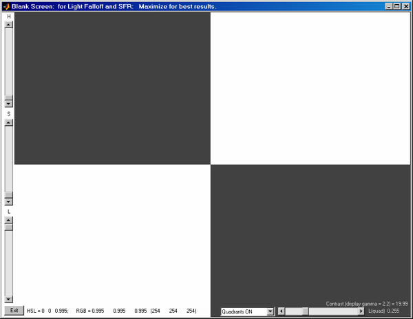
Screen Patterns Quadrants display set for 20:1 contrast.
Screen Patterns offers a number of options; for example, the highlight Hue, Lightness, and Density can be adjusted so you can photograph a variety of colors. SFR: Quads: Global H,S sets the H (Hue) and Saturation (S) levels in the quadrants to the same values as the highlight region so you can obtain single-color patterns.
Web page pattern
The test pattern below is dark gray and white rather than black and white because LCD screens
can have extremely high contrast-- 400:1 or more-- enough to cause clipping,
which reduces the accuracy of Imatest SFR measurements.
|
When you display this taget
on a LCD screen, be sure to maximize the browser window. To avoid Moire
fringing (interference between the LCD and camera sensor pixels) and chromatic
aberration from the R-G-B pixel pattern, the LCD screen image should take
up no more than 1/3 to 1/4 the width of the total image (1/9 to 1/16 the
area).
My inexpensive Toshiba laptop, shown on the right, displays 1024 pixels
horizontally. The Canon EOS-10D has 3072 horizontal pixels. In this case,
the laptop image should take up no more than 1/4 the image width.
|
|
Since the screen occupies only a small portion of the image area, be sure the camera is focused on the screen!
The first two zones are 1000
pixels high; the remaining zones are 600 pixels high. Scroll down to locate
the edge of choice.
The pattern contrast was reduced slightly on August
1, 2004.
Return to Imatest SFR instructions
SFR results: MTF (Sharpness) plot
If you entered Imatest on this page, you may want to explore the background information in these links.
Sharpness introduces sharpness measurements and MTF.
Sharpening describes Standardized sharpening.
How to test Lenses with Imatest contains conscise instructions on testing lenses.
Image quality factors lists the factors measured by Imatest.
Imatest SFR displays Edge profiles and SFR (Spatial frequency response) plots with spatial frequency labelled in
- Cycles per Pixel (C/P) or Cycles per distance (inches or mm), and/or
- Line widths per picture height (LW/PH; shown below),
depending on the checkbox settings of the first two lines of the Plot section of the SFR input dialog box , shown below.
The LW/PH box is unchecked by default. Note that one cycle (or line pair) is equivalent to two line widths.
Important results below are shown in Bold. The most important is MTF50, without and with Standardized sharpening. Its relationship with print quality is discussed in Interpretation of MTF50. The contents of the plots are affected by whether or not Standardized sharpening is checked in Settings section of the SFR input dialog box. Differences in plot content are indicated by [Std Sharpening checked] or [Std Sharpening off].
Edge response
Upper left: Spatial domain plot |
 Edge profile [Standardized sharpening on]
 |
| Black line (bold) |
Edge profile for the luminance (Y) channel, where Y = 0.3*R + 0.59*G + 0.11*B. Original (without standardized sharpening).
The edge profile shown on the right is proportional to the light intensity. You may also select to display the Line Spread Function (LSF; the derivative of the edge profile), shown on the right, below, or Pixel levels (which includes gamma-encoding). |
Red line
(dashed, bold) |
Edge profile for the luminance (Y) channel with standardized sharpening, indicated by (corr) for "corrected." Radius R used for setting standardized sharpening is displayed. Defaults to 2, but may set manually; may be larger for unusually broad transitions (poor MTF response). [Std Sharpening checked] |
R, G, B
dashed lines (thin) |
Individual edge profiles for R, G, and B channels. Shown more prominently in the Chromatic Aberration plot, below. Barely visible in this illustration because this camera has very little chromatic aberration. Imatest Master only. |
Left column text
(input settings) |
| Title, including measurement orientation. (A vertical edge is used for a horizontal profile.) |
| Image height (H) or Width x Height (WxH) in pixels |
| Total megapixels |
| Channel. Defaults to Y (luminance). R, G, or B are also available. |
| Gamma is an estimate of camera gamma used to linearize the image. Defaults to 0.5. |
| Region of interest (ROI) size in pixels |
| ROI location in percentage of distance from center to corner. |
|
Right column text
(results) |
| [not for LSF] 10-90% rise distance (original; uncorrected) in pixels and rises per picture height (PH). |
 Line spread function [Std Sharpening off]
|
| [not for LSF] 10-90% rise distance (with standardized sharpening; indicated by (corr) for "corrected") in pixels and rises per PH. Radius R used for setting standardized sharpening is displayed. Defaults to 2, but may set manually; may be larger for unusually broad transitions (poor MTF response). Includes the equivalent "ideal megapixels" in brackets [...]. [Std Sharpening checked; not for LSF] |
| [not for LSF; Imatest Master only] 10-90% rise distances of the R, G, and B channels, individually. Imatest Master only. |
| [LSF only] Peak LSF (maximum d(Edge)/dx) and PW50 (50% pulse width) in pixels and pulse widths per picture height (PH). |
| RMS edge roughness in pixels. A promising measurement related to image quality. Shown on the right. [Std Sharpening off] |
| Overshoot and undershoot. Percentage of step amplitude. Shown if appropriate. [Std Sharpening checked] |
| Average pixel levels in dark and light areas, and light/dark ratio. Clipping can occur if they are too close to 0 or 255. Also gives the ratio between the light and dark areas: an indication of the contrast of the image. |
|
Spatial Frequency Response (MTF)
Lower left:
Frequency domain (MTF) plot |
|
| Black line (bold) |
Spatial Frequency Response (MTF) for the luminance (Y) channel. Unprocessed. |
Red line
(dashed,bold) |
Spatial Frequency Response (MTF) for the luminance (Y) channel with Standardized sharpening. [Std Sharpening checked] |
Right column text
(results) |
| MTF50
(50% contrast spatial frequency) for the original uncorrected image in cycles/pixel and line widths per picture height (LW/PH). Its relationship to print quality is discussed in Interpretation of MTF50. |
| MTF50
(with standardized sharpening; corrected) in cycles/pixel and
LW/PH. Radius R used for setting standardized sharpening is displayed.
Defaults to 2 (larger for unusually broad transitions (poor
MTF response)). It may be adjusted in the input dialog box. [Std Sharpening checked] |
| Equivalent "ideal megapixels" in brackets [n mpxls ideal]: a number
based on the concept that the "ideal" pixel would have an MTF of 1 up to
the Nyquist frequency (0.5 C/P), and 0 above, and hence, MTF50 = 0.5 C/P.
The number of "ideal pixels" that would yield the identical sharpness (MTF50) is, |
|
4 * MTF50(C/P horizontal) * horizontal pixels * MTF50(C/P vertical) * vertical
pixels |
| The number displayed assumes
that MTF50 is the same in horizontal and vertical directions— usually, but not always,
a good assumption—
there are exceptions, such as the Nikon D70. You should not expect the
"ideal megapixel" count to equal the total megapixel count of the camera.
In the real world, performance is excellent if it is half the actual megapixels. In cameras with weak anti-aliasing filters or a high degree of sharpening, MTF may be greater than 0.5 at the Nyquist frequency. In this case, [> n mpxls ideal] is displayed, where n is the total number of pixels in the camera, is displayed. Larger numbers are meaningless. Aliasing issues such as moire patterns may be present, but the simple slanted edge pattern cannot be used to evaluate the seriousness of aliasing. |
|
| MTF50P
(spatial frequency where contrast is 50% of its peak value) for the original uncorrected image in cycles/pixel and line widths per picture height (LW/PH). This is the same as MTF50 for slightly to moderately sharpened edges, but smaller for oversharpened edges. It may be a better indicator than MTF50 of the perceived sharpness of oversharpened images. [Std Sharpening off] |
| Oversharpening or undersharpening. The amount the camera is over- or undersharpened with respect to standardized
sharpening. 100% ( MTF( feql ) - 1) where feql is the frequency where MTF is set to 1 by standardized sharpening. [Std Sharpening checked] |
| MTF30 (30% contrast spatial
frequency for the original uncorrected image) is the default value of the Secondary Readout, which can be set in the SFR input dialog window. You can select MTFxx, the spatial frequency for xx% contrast, or the MTF at a spatial frequency specified in cycles/pixel, pixels/mm, or pixels/inch. |
| MTF at the Nyquist
frequency. May indicate of the effectiveness of the anti-aliasing filter and
likelihood
of aliasing effects such as Moire patterns. But it not an unambiguous indicator because aliasing is related to sensor response, and MTF at Nyquist is the product of sensor response, the de-mosaicing algorithm, and sharpening, which can boost response at Nyquist for radii less than 1. Aliasing effects may become serious over 0.3. There is a tradeoff: the
more
effective the sensor anti-aliasing, the worse the sharpness. Foveon sensors
(used in the Sigma SD9 and SD10) are more tolerant of aliasing than Bayer sensors, which are used in most digital cameras. |
| Nyquist frequency: Half
the sampling rate = 1/(2*pixel
spacing). Always 0.5 cycles/pixel. Indicated by the vertical blue line. |
|
Input data
| Right: Input data |
 |
| |
Top right image
Thumbnail of the entire image, showing the location of the selected region of interest (ROI) in red.
|
| |
Middle right image
The selected region of interrest (ROI), shown with the correct aspect ratio, but not necessarily the exact size. The following parameters are displayed below the image.
-
ROI size in pixels
- ROI boundary locations (Left, Right, Top, and Bottom) in pixels from the upper-left corner,
- Edge angle in degrees, and
- Estimated chart contrast, derived from the average pixel levels of the light and dark areas (away from the transition) and gamma. The equation: Estimated chart contrast = (avg. pixel level of light area/avg. pixel level of dark area)^(1/gamma)
|
| |
Lower right text
Selected EXIF data: Data recorded by the digital camera. Only for JPEG files. May include ISO speed, aperture, and other details. Thanks to Matthias Wandel for jhead.exe.
|
SFR results: Chromatic Aberration, Noise, and Shannon capacity plot
Chromatic Aberration, noise, and Shannon capacity
The camera chosen for the plot below has significant Chromatic Aberration. The Noise spectrum and
Shannon capacity plots, shown below beneath Chromatic Aberration,
are plotted only if the Noise Spectrum and Shannon capacity (in CA plot) checkbox in the Imatest SFR input dialog box has been checked. It is unchecked by default.
| Upper plot: Chromatic Aberration |
|
| More about this plot can be found in the page on Chromatic Aberration. Much of this plot is grayed out if the ROI is too close to the center for reliable CA measurements (less than 30% of the distance to the corner). |
Red, Green, and Blue
lines (bold) |
Edge profiles for the R, G, and B channels (original, uncorrected). (Standardized sharpening is not used for chromatic aberration.) |
| Black line (dashed) |
Edge profile for the luminance (Y) channel. |
| Dashed magenta line (bold) |
The difference between the highest and lowest channel levels. (All channels are normalized to go from 0 to 1.) The visible chromatic aberration is proportional to the area under this curve. |
| Left column text |
Input settings: Plot title, profile orientation (Horizontal profile corresponds to a vertical edge, etc.), image dimensions (WxH), total megapixels, gamma, ROI size, ROI location. |
Right column text
(results) |
| 10-90% rise distance (original; uncorrected) in pixels and rises per picture height (PH). |
| CA (area): Chromatic aberration area in pixels. An indicator of the severity of CA. The area between the channels with the highest and lowest levels. In units of pixels because the x-axis is in pixels and the y-axis is normalized to 1. Explained in the page on Chromatic aberration. Meaning (now obsolete): Under 0.5; insignificant. 0.5-1: minor; 1-1.5: moderate; 1.5 and over: serious. |
| CA: Chromatic aberration as a percentage of center-to-corner distance. A better indicator than pixels (above). Equal to 100 * (CA in pixels) / (distance from center in pixels), corrected for the edge angle. Relatively independent of the ROI location because CA tends to be proportional to the distance from the image center. It is also independent of the number of pixels in the sensor. Explained in the page on Chromatic aberration. Appxoximate meaning: Under 0.04; insignificant. 0.04-0.08: minor; 0.08-0.15: moderate; over 0.15: serious. |
| CA (crossing): Chromatic aberration based on the edge centers (where the edges cross 0.5). This is generally smaller than CA (equiv.) and also less indicative of the visibility of the CA. This measurement can be very different from CA (area) due to the effects of demosaicing. It is usually very close when Bayer RAW images are analyzed. |
| R-G, B-G :Red-Blue and Red-Green spacings in percentage of center-to-corner distance. Useful for correcting CA, especially when applied prior to demosaicing. Displayed only in Imatest Master. |
| Average pixel levels in the dark and light areas. Clipping can occur if they are too close to 0 or 255. |
|
Below
the
plot |
These items are only displayed if the Noise Spectrum and Shannon capacity box is unchecked.
Noise in the dark and light
areas, described below.
A thumbnail of the image showing the region of interest (ROI). |
Lower part of figure: Noise and Shannon information capacity plots
for for the selected channel, normally luminance (Y)
Shannon capacity is an experimental measurement that is strongly affected by signal processing (especially sharpening and noise reduction). It is not a reliable way of quantifying camera performance. |
Noise spectrum plot
(left side) |
The noise spectrum plot
is somewhat experimental. Bayer interpolation causes the noise spectrum to roll off to about 0.5 at 0.5 Cycles/Pixel; noise reduction causes additional rolloff.
Low to middle frequency noise components tend to be more visible. The spiky light cyan
and green curves represent two different
directions.
The thick black line is the smoothed average of the two. The red line is a third order polynomial fit to the noise. |
Noise spectrum and Shannon capacity are only plotted if the selected region is large enough to provide reasonable noise statistics.
 |
Shannon capacity plot
(right sde) |
Shannon capacity C
as a function of signal S (closely related to image Contrast), where S is expressed as the percentage of the difference between the white
and black regions of the target (Sstd ). A Contrast of 100% represents a fairly contrasty image, 10% represents
a low contrast image, and 1% represents a smooth area like skies. These numbers
are only meaningful for comparing digital cameras. They should be used with caution because signal processing, especially noise reduction, has a strong effect on Shannon Capacity. There is
a table of results in the page on Shannon
information capacity. |
| Text at bottom |
| Noise in the dark and light
areas, and the mean of the two. Measured after the input data has been
linearized (corrected for the gamma encoding). Expressed as a fraction
of the difference between the average levels of the light and dark areas (Sstd ).
This difference is the standard signal, S, used in the calculation of Shannon
information capacity. The noise measurements in Q-13 Stepchart and Colorcheck are more reliable and useful. |
| Signal-to-noise ratio S/N
for the mean of the light and dark areas. This is the inverse of the noise
for the mean of the light and dark areas, above. Used in the calculation
of Shannon capacity. |
| Shannon
information capacity of the camera for signal S =
Sstd,
measured in bits per pixel and megabytes total. This is an approximate
calculation that provides an estimate of overall image quality for moderately
contrasty images, as affected by sharpness and noise. |
|
SFR results: Multiple ROI (Region of Interest) plot
Imatest SFR allows you to
select several regions of interest (ROIs) in an image. Display options from the SFR input dialog box are shown below.
When one of the Multi-ROI plots (1D or 2D; Cycles/pixel or LW/PH) has been selected, one of the two composite multiple ROI plots shown below is produced. The 1D summary plots, which display MTF, rise distance, and chromatic aberration as a function of the distance from the image center, may be difficult to read for lenses that are poorly centered and hence have asymmetrical response. In such cases the 2D summary plots are far more readable.
Starting with Imatest 2.6 (January 2008) a number of new options facilitate editing and refining multiple ROI selections. They are described here. You can also create Excel plots that summarize results from several multi-ROI runs, as shown on the right using the procedure given here. |
|
2D summary plot
When one of the 2D images (Cy/Pxl or LW/PH) are selected, the image below is displayed. It shows the regions of interest (ROI) and the following parameters for each ROI.
N (ROI number): Center-corner distance in %
MTF50 Cycles/Pixel or LW/PH (displayed boldface for emphasis)
MTF20 Cycles/Piexl or LW/PH
Chromatic Aberration (area in pixels)
The dotted circles delimit the central region (up to 30% of the center-to-corner distance), the part-way region, and the corner region (over 75% of the center-to-corner distance). The New Weighted MTF50 is the weighted mean of the mean MTFs in the three areas, where the weights are 1 (Central), 0.75 (part-way), and 0.25 (corner).
Multi-ROI 2D summary plot, showing Center-corner distance,
MTF50, MTF20, and CA superimposed on image.
This display, introduced with Imatest 2.5.8 (January 2008), can be particularly useful because lenses are not always centered properly. If they were, performance would be a simple function of the distance from image center. You can quickly review the summary results, then look at the detailed results for individual regions. It was developed because about 9 regions (center, 4 - part-way out, 4 - corner) is sufficient to characterize lens performance, but not sufficient for a meaningful 2D or 3D contour plot (which requires about 20 regions). Also, contour plots can only show one parameter (e.g., MTF50), while this display shows several.
1D Summary plot showing results as a function of distance from the center
This figure contains two plots: MTF50 (upper left) and 10-90% rise distance (lower left). If Cycles/pixel is selected, units are relative to pixels; if LW/PH is selected, units are relative to image height. These figures show performance (MTF50 and rise distances without
and with standardized sharpening). The Cycles/pixel Figure also plots Chromatic
Aberration as a function of distance from the center of the image, scaled as the percentage of distance from center to corner (0 = center; 1 = corner).
The most important results below are shown in Bold. Illustrations are for the first figure (Cycles per pixel in this case).
| Upper left: MTF50 (Half-contrast frequency)
|
|
| This plot shows MTF50 (the half-contrast spatial frequency) as a function of distance from the center of the image, scaled as the percentage from center to corner (0 = center; 100 = corner). There are two vertical (y) axes. The primary axis is on the left; the secondary axis (italicized) is on the right. These alternate for the two plots. In this plot, the primary axis is in Cycles/pixel for MTF50 and Pixels for 10-90% rise distance. It can also be in Cycles/mm or Cycles/inch if specified in the SFR data window. |
Black line (bold) |
MTF50 (half-contrast spatial frequency) for the luminance (Y) channel. Unprocessed. This is the number to use for measuring lens sharpness. |
Red line
(bold, dashed) |
MTF50 for the luminance (Y) channel with Standardized sharpening. This is the number to use when making general comparisons of different cameras with different degrees of sharpening. |
Symbols and numbers
below data points,
top to bottom |
| Orientation: Location of region relative to image center. A = Above, B = Below, L = Left, R = Right. |
| MTF50, Uncorrected and with Standardized sharpening, in units corresponding to the primary vertical (y) axis scale on the left. The vertical order is determined by the order of the data points, i.e., if the Uncorrected MTF50 is higher, its value is on top. |
| MTF50, Uncorrected and with Standardized sharpening, in units corresponding to the secondary vertical (y) axis scale on the right. These numbers are italicized. The vertical order is determined by the order of the data points, i.e., if the Uncorrected MTF50 is higher, its value is on top. |
|
| Right column: Crop, Results summary, and EXIF data |
Top right image
Thumbnail of the entire image, showing the locations of the selected regions of interest (ROI) in red.
|
Middle right box:
Weighted MTF50
Results summary
|
Summary of key results of multiple ROI runs:
Weighted mean values for MTF50, in cycles per ... and LW/PH units, without and with standardized sharpening. The MTF value at the middle of each (sorted) line segment is weighted according to the length of the line segment and the distance from the center: the center is weighted twice as strongly as the corner. These weights are used to calculate a weighted mean. This algorithm prevents closely spaced points from being given excessive weight. |
Lower right text
Selected EXIF data: Data recorded by the digital camera. Only for JPEG files. May include ISO speed, aperture, and other details. Thanks to Matthias Wandel for jhead.exe. |
|
 |
|
Lower left: 10-90% Edge
rise distance
|
 The Legend at the lower right of the 10-90% Rise distance plot sometimes covers data points. It can be moved by clicking and dragging it with a mouse.
 |
|
Black line
(bold)
|
The 10-90% rise distance,
uncorrected (without Standardized sharpening). |
|
Red
line
(bold,
dashed)
|
The 10-90% rise distance, with Standardized sharpening. |
|
.Blue
line
(bold,
dashed)
with
yellow
circles.
|
Chromatic
aberration (Area-based) in pixels. An indicator of the severity
of CA. The area between the channels with the highest and lowest levels.
In units of pixels because the x-axis is in pixels and the y-axis is normalized
to 1. Explained in detail in the page on
Chromatic
aberration. Meaning: Under 0.5; insignificant. 0.5-1: minor;
1-1.5: moderate; 1.5 and over: serious. |
When the SQF (multi) checkbox in the SFR input dialog box has been checked, a multiple ROI SQF Figure is produced.
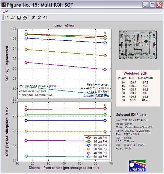
The upper plot shows SQF without standardized sharpening (unprocessed) for picture heights from 10 to 60 cm. The lower plot shows SQF with standardized sharpening (R = 2). Weighted SQFs are shown in the table on the right. The weighting formula is the same as the one used for MTF: readings near the center are given twice the weight of readings near the edge.
CSV output file
The CSV output file has been upgraded (version 2.6.1, January 2008) to facilitate the handling of a large volume of results and creation of Excel summary plots that combine results of several runs. It is designed to be opened in Excel. The following data shows the contents of the CSV file for the Canon 17-85 IS lens tested on the EOS-40D. It has been imported from Excel. |

Summary plot
|
Header shows version, input file, and run date
| Imatest |
2.6.1 |
Pro |
SFR multi-ROI |
| File |
85mm_f5.6_IMG_5970.JPG |
|
| Run date |
1/9/2008 10:25 |
|
|
Geometry & file shows the Regions of interest (ROIs) in pixels and the CSV summary files for each location.
| Geometry & file: changed with Imatest 2.5.8. Origin at upper left. |
|
|
|
| N |
Distance % |
Direction |
X1 |
Y1 |
X2 |
Y2 |
Region |
CSV summary file |
| 1 |
12.1 |
AL |
1749 |
922 |
1894 |
1161 |
Center |
D:\Camera_tests\Canon_EOS-40D\17-
85_IS\Results\85mm_f5.6_IMG_5970_YAL12_MTF.csv |
| 2 |
38.7 |
BL |
1244 |
1839 |
1380 |
2044 |
Pt Way |
D:\Camera_tests\Canon_EOS-40D\17-
85_IS\Results\85mm_f5.6_IMG_5970_YBL39_MTF.csv |
| 3 |
38.3 |
AL |
1221 |
577 |
1355 |
798 |
Pt Way |
D:\Camera_tests\Canon_EOS-40D\17-
85_IS\Results\85mm_f5.6_IMG_5970_YAL38_MTF.csv |
| 4 |
36.1 |
AR |
2432 |
551 |
2575 |
781 |
Pt Way |
D:\Camera_tests\Canon_EOS-40D\17- 85_IS\Results\85mm_f5.6_IMG_5970_YAR36_MTF.csv |
| 5 |
36.2 |
BR |
2446 |
1817 |
2576 |
2032 |
Pt Way |
D:\Camera_tests\Canon_EOS-40D\17-
85_IS\Results\85mm_f5.6_IMG_5970_YBR36_MTF.csv |
| 6 |
90 |
AL |
104 |
52 |
238 |
279 |
Corner |
D:\Camera_tests\Canon_EOS-40D\17-
85_IS\Results\85mm_f5.6_IMG_5970_YAL90_MTF.csv |
| 7 |
89.9 |
BL |
133 |
2364 |
273 |
2579 |
Corner |
D:\Camera_tests\Canon_EOS-40D\17-
85_IS\Results\85mm_f5.6_IMG_5970_YBL90_MTF.csv |
| 8 |
87.3 |
BR |
3571 |
2333 |
3696 |
2544 |
Corner |
D:\Camera_tests\Canon_EOS-40D\17-
85_IS\Results\85mm_f5.6_IMG_5970_YBR87_MTF.csv |
| 9 |
87.1 |
AR |
3550 |
30 |
3686 |
251 |
Corner |
D:\Camera_tests\Canon_EOS-40D\17-
85_IS\Results\85mm_f5.6_IMG_5970_YAR87_MTF.csv |
nroi – roi_mult These four lines are used to define the regions in imatest.ini. These regions can be reused for Imatest runs by copying and pasting the four lines into imatest.ini, replacing the previous lines. Imatest.ini can be opened for editing by clicking Settings (in the Imatest main window), View settings (ini file).
| nroi = 9 |
| nwid_save = 3888 |
| nht_save = 2592 |
| roi_mult = 1749 922 1894 1161 ; 1244 1839 1380 2044 ; 1221 577 1355 798 ; 2432 551 2575 781 ; 2446 1817 2576 2032 ; 104 52 238 279 ; 133 2364 273 2579 ; 3571 2333 3696 2544 ; 3550 30 3686 251 ; |
Primary results, shown by region
| Primary results |
|
|
|
|
|
|
|
| N |
MTF50 (Cy/Pxl) |
R1090
(pxl) |
CA
(pxl) |
MTF50
(LW/PH) |
R1090
(/PH) |
Peak
MTF |
MTF50P
(Cy/Pxl) |
MTF50P
(LW/PH) |
| 1 |
0.289 |
1.6499 |
0.3439 |
1498.2 |
1571 |
1 |
0.289 |
1498.2 |
| 2 |
0.2938 |
1.8284 |
0.3155 |
1522.9 |
1417.6 |
1 |
0.2938 |
1522.9 |
| 3 |
0.2566 |
2.1939 |
0.3113 |
1330.1 |
1181.5 |
1 |
0.2566 |
1330.1 |
| 4 |
0.2821 |
1.7768 |
1.0413 |
1462.5 |
1458.8 |
1 |
0.2821 |
1462.5 |
| 5 |
0.2993 |
1.6187 |
1.0377 |
1551.3 |
1601.3 |
1 |
0.2993 |
1551.3 |
| 6 |
0.1884 |
2.7046 |
1.0397 |
976.5 |
958.4 |
1.0201 |
0.1857 |
962.6 |
| 7 |
0.1871 |
2.5718 |
1.0671 |
969.9 |
1007.8 |
1.0239 |
0.1834 |
950.8 |
| 8 |
0.2191 |
2.3951 |
1.835 |
1135.8 |
1082.2 |
1.0132 |
0.2171 |
1125.7 |
| 9 |
0.3017 |
1.8871 |
1.6025 |
1563.8 |
1373.5 |
1.0104 |
0.3004 |
1557 |
</
Summary results The table contains summary results. These results are repeated in a single-column at the end of the CSV file, shown below. Though it is less readable, it is much better suited for copying and pasting summary results into an Excel file that can be used to produce plots.
| Summary |
1/9/2008
10:25 |
|
85mm_f5.6_IMG_5970.JPG |
|
|
|
|
|
| 9 |
Regions |
1 |
Center |
4 |
Part way |
4 |
Corner |
|
|
|
| |
MTF50
(Cy/Pxl) |
R1090
(pxl) |
CA
(pxl) |
MTF50
(LW/PH) |
R1090
(/PH) |
Peak
MTF |
MTF50P
(Cy/Pxl) |
MTF50P
(LW/PH) |
MTF20
(Cy/Pxl) |
MTF20
(LW/PH) |
| Mean Ctr |
0.289 |
1.6499 |
0.3439 |
1498.2 |
1571 |
1 |
0.289 |
1498.2 |
0.3598 |
1865.4 |
| Mean Pt Wy |
0.2829 |
1.8544 |
0.6765 |
1466.7 |
1414.8 |
1 |
0.2829 |
1466.7 |
0.3626 |
1879.6 |
| Min Pt Wy |
0.2566 |
1.6187 |
0.3113 |
1330.1 |
1181.5 |
1 |
0.2566 |
1330.1 |
0.343 |
1778.2 |
| Mean Cor |
0.2241 |
2.3897 |
1.3861 |
1161.5 |
1105.5 |
1.0169 |
0.2216 |
1149 |
0.323 |
1674.2 |
| Min Cor |
0.1871 |
1.8871 |
1.0397 |
969.9 |
958.4 |
1.0104 |
0.1834 |
950.8 |
0.2778 |
1440 |
| Wtd mean |
0.2786 |
1.8191 |
1.1495 |
1444.3 |
1454.2 |
1.0021 |
0.2783 |
1442.7 |
0.3563 |
1846.8 |
Explanation of summary results Each of the results are presented six times— for different regions of the image and for a weighted sum of the regions, as described below.
| Mean Ctr |
The mean of the central region (Ctr), up to 30% of the center-to-corner distance. |
| Mean Pt Wy |
The mean of the Part-Way region (Pt Wy), from 30 to 75% of the center-to-corner distance. |
| Min Pt Wy |
The minimum value of the Part-Way region. If the minimum value is much below the mean, the lens may be poorly centered (due to manufacturing tolerances). |
| Mean Cor |
The mean of the corner region, which is over 75% of the center-to-corner distance. |
| Min Cor |
The minimum value of the corner region. If the minimum value is much below the mean, the lens may be poorly centered (due to manufacturing tolerances). |
| Wtd mean |
The weighted mean. For all parameters except chromatic aberration (CA (pxl)) the weights are 1 for Ctr, 0.75 for Pt Wy, and 0.25 for Cor. For CA (pxl) the weights are 1 for Cor and 0.5 for Pt Wy. (Lateral chromatic aberration is not important near the center.) |
The column in this table (rows in the single-column table below) contain the following results:
| MTF50
(Cy/Pxl) |
The spatial frequency where MTF is 50% (0.5) of its low frequency value.
Normally in cycles/pixel, but may be in cycles/mm or cycles/in if specified in SFR input dialog box. |
| R1090
(pxl) |
The 10-90% rise distance in pixels. |
| CA
(pxl) |
Chromatic Aberration (expressed in area between highest and lowest channel) in pixels. |
| MTF50
(LW/PH) |
MTF50 expressed in Line Widths per Picture Height, where 1 line pair = 2 line widths. (LW/PH is traditional in video.) |
| R1090
(/PH) |
The number of 10-90% rises per picture height. |
| Peak
MTF |
The peak value of MTF. Equal to 1 when little or no sharpening is applied; can be much larger than 1 when strong sharpening is applied. |
| MTF50P
(Cy/Pxl) |
The spatial frequency where MTF is 50% of the peak value. Differs from MTF50 when strong sharpening is applied. |
| MTF50P
(LW/PH) |
MTF50P expressed in Line Widths per Picture Height. |
| MTF20 (Cy/Pxl) |
The spatial frequency where MTF is 20% (0.2) of its low frequency value.
Normally in cycles/pixel, but may be in cycles/mm or cycles/in if specified in SFR input dialog box. |
| MTF20
(LW/PH) |
MTF30 expressed in Line Widths per Picture Height. |
Secondary results These include results with standardized sharpening (suffix C).
| Secondary results: C denotes standardized sharpening |
|
|
| N |
MTF50C
(Cy/Pxl) |
R1090C
(pxl) |
MTF50C
(LW/PH) |
R1090C
(/PH) |
MTF20
(Cy/Pxl) |
MTF20
(LW/PH)
|
| 1 |
0.294 |
1.5689 |
1524.2 |
1652.1 |
0.3598 |
1865.4 |
| 2 |
0.3013 |
1.5304 |
1561.9 |
1693.7 |
0.374 |
1939.1 |
| 3 |
0.2841 |
1.594 |
1472.7 |
1626.1 |
0.343 |
1778.2 |
| 4 |
0.2977 |
1.5477 |
1543.1 |
1674.8 |
0.3604 |
1868.2 |
| 5 |
0.304 |
1.5129 |
1575.9 |
1713.3 |
0.3729 |
1933.1 |
| 6 |
0.2245 |
2.0172 |
1163.7 |
1285 |
0.2778 |
1440 |
| 7 |
0.2271 |
1.9317 |
1177.3 |
1341.8 |
0.3191 |
1654.4 |
| 8 |
0.281 |
1.625 |
1456.5 |
1595.1 |
0.316 |
1638 |
| 9 |
0.3188 |
1.441 |
1652.5 |
1798.7 |
0.379 |
1964.5 |
Miscellaneous values
| Image WxH & Mpxls |
3888 |
2592 |
10.1 |
| Channel |
Y |
|
|
| Gamma |
0.5 |
|
|
| Sharpening radius |
2 |
|
|
| Pixels per inch |
|
|
| Pixels per mm |
|
|
| um per pixel |
|
|
| MTF50 wtd Cy/Pxl (uncorr) |
0.278 |
|
|
| MTF50 wtd LW/PH (uncorr) |
1440 |
|
|
| MTF50 wtd Cy/Pxl (corr) |
0.294 |
|
|
| MTF50 wtd LW/PH (corr) |
1525 |
|
|
SQF summary. SQF is the Subjective Quality Factor, described here.
| SQF (Subjective Quality Factor): mean values |
Print
height |
Viewing
dist (cm) |
SQF |
SQF_corr |
| 1 |
15 |
99.58 |
99.76 |
| 2 |
15 |
98.98 |
99.66 |
| 3 |
16.43 |
98.45 |
99.62 |
| 4 |
18.97 |
98.1 |
99.55 |
| 5 |
21.21 |
97.75 |
99.45 |
| 6 |
23.24 |
97.39 |
99.32 |
Exif data
| Exif data |
| File: 2008:01:02 10:34:42 |
| Make: Canon |
| Model: Canon EOS 40D |
| Taken: 2008:01:02 10:34:42 |
| Res: 3888 x 2592 |
| FL: 85.0mm |
| CCD: 22.25mm |
| Exp: 0.200 s (1/5) |
| Aper: f/5.6 |
| ISO: 100 |
| ExBias: 0.67 |
| WtBal: Auto |
Creating Excel plots
The single column summary is the last table in the multi-ROI CSV file. It contains the same data as the summary results (above), but it is formatted so it can be easily copied and pasted into another Excel file for creating plots that summarize several runs. For mult-ROI batch runs, this data is combined into a CSV output file with a name of the form, filename_Y_sfrbatch.csv.
Summary plot for 6 multi-ROI runs (f/5.6-f/32) for the Canon 17-85mm IS lens on the EOS-40D (JPEG)
The Excel file was created by combining single-column summary results from the 6 runs.
Any of the parameters in the summary can be plotted. To obtain a plot,
- Run a sequence of multi-ROI runs for a several apertures (or other settings if appropriate). If possible, select one ROI near the center, 4 part-way out, and 4 near the corners: 9 total as shown in the 2D summary plot, above. This is sufficient to completely characterize a lens. Be sure to save the CSV summary file, which has a name of the form {input file name}_Y_multi.csv, where Y denotes the luminance channel.
- If the sequence is run as a batch, a combined summary file with a name of the form filename_Y_sfrbatch.csv will be created. You may skip the next four steps.
- Open the first CSV smmary file (for f/5.6 in this case) in Excel. This can usually be done by double-clicking on the file name in Windows Explorer.
- Select and copy (ctrl-C) the first two columns of the summary results, located near the end of the CSV summary file.
- Open a new Excel (XLS) file. Paste the selection in the new file.
- Open the remaining CSV summary files in Excel. For each file, copy the second column of summary data, and paste it into the next Excel file so that it is aligned with the previous data, as shown above.
- In the row 2 of the new Excel file, between Summary results... and Date, (or the line labeled Plot title in the combined summary file) enter a brief description of the run to be used to label the plot, for example, f/5.6, f/8, ..., f/32 (shown above).
- Now you can create the plot. Select the cells for the x and y-displays. The remaining details depend on your version of Excel. For the above plot, the range of data is
=Sheet1!$A$2:$G$2,Sheet1!$A$65:$G$65 .
Single-column summary results
(imcomplete)
The parameters in the table are described here. |
|
| Summary results in single column for copying and creating plots |
| |
(enter description here) |
| Date |
1/9/2008 10:25 |
| File |
85mm_f5.6_IMG_5970.JPG |
| Regions |
9 |
| Center |
1 |
| Part way |
4 |
| Corner |
4 |
| |
|
| MTF50 (Cy/Pxl) Mean Ctr |
0.289 |
| R1090 (pxl) Mean Ctr |
1.6499 |
| CA (pxl)) Mean Ctr |
0.3439 |
| MTF50 (LW/PH) Mean Ctr |
1498.2 |
| R1090 (/PH) Mean Ctr |
1571 |
| Peak MTF Mean Ctr |
1 |
| MTF50P (Cy/Pxl)) Mean Ctr |
0.289 |
| MTF50P (LW/PH) Mean Ctr |
1498.2 |
| MTF20(Cy/Pxl) Mean Ctr |
0.3598 |
| MTF20 (LW/PH) Mean Ctr |
1865.4 |
| |
|
| MTF50 (Cy/Pxl) Mean Pt Wy |
0.2829 |
| R1090 (pxl) Mean Pt Wy |
1.8544 |
| CA (pxl)) Mean Pt Wy |
0.6765 |
| MTF50 (LW/PH) Mean Pt Wy |
1466.7 |
| R1090 (/PH) Mean Pt Wy |
1414.8 |
| Peak MTF Mean Pt Wy |
1 |
| MTF50P (Cy/Pxl)) Mean Pt Wy |
0.2829 |
| MTF50P (LW/PH) Mean Pt Wy |
1466.7 |
| MTF20(Cy/Pxl) Mean Pt Wy |
0.3626 |
| ..., etc. (The whole table is not shown.) |
|
Using SFRplus Part 1
Setting up and photographing the SFRplus target
Imatest SFRplus
performs highly automated measurements of several key image quality factors using a specially-designed test chart. Unlike other modules, the user never has to manually select Regions of Interest (ROIs). Image quality factors include
SFRplus operates in two modes.
- Interactive/setup mode, which allows you to set up region selection and calculation parameters and interactively examine results in detail.
- Auto mode, which runs automatically with no additional user input. ROIs are selected automatically based on settings saved from the interactive/setup mode. This allows images of different sizes and framing to be analyzed with no change of settings. Auto mode is especially useful for rapid automated testing, where framing varies from image to image.
This document introduces SFRplus and explains how to obtain and photograph the chart. Part 2 shows how to run SFRplus inside Rescharts and how to save settings for automated runs. Part 3 illustrates the results.
The SFRplus
test chart
The standard SFRplus test chart is illustrated below.
Standard SFRplus test chart: 5x9 grid, 10:1 and 2:1 contrasts,
with 20-step 4x5 stepchart
(0.1 density increment).
Sharpness is derived from light-to-dark slanted edges at the boundaries of the squares, as described in Sharpness:
What is it and how is it measured? The new chart enables SFRplus can handle a wide range of camera aspect ratios; the left and right sides of the chat can extend beyond the frame or be well-inside the frame.
Advantages of the SFRplus chart over the ISO 12233 chart
- Much less wasted area. About 90% of the ISO chart is covered with patterns that have little value for computer analysis.
- You can produce a map of sharpness (MTF) over the image surface (up to 23 regions). This cannot be done with the ISO chart because there are only a few suitable edges— and they may not be well-located.
- The 10:1 contrast edges are less likely to clip than the edges in the ISO chart, which is specified to have a contrast of at least 40:1. The camera operates in a more linear region, and hence results are more consistent and accurate— less affected by overexposure and underexposure. Also, 10:1 edges are more representative of real edges that affect perceived image sharpness.
- The low contrast edges provide additional information about signal processing in the camera under test. Although Imatest SFR is relatively insensitive to chart contrast (MTF is normalized to 100% at low spatial frequencies), measured SFR is often affected by chart contrast due to nonlinear signal processing in cameras, as described in the box below.
- The SFRplus chart is well-suited for automated testing (yes, with SFRplus)! With the ISO chart, regions of interest (ROIs) must be selected carefully whenever the image framing changes— even slightly.
- The measurement is ISO-compliant. ISO-compliant measurements do not require the standard ISO chart. The upcoming revision to the ISO standard will recommend an entirely different pattern of low contrast.
- It can measure additional image quality factors, including distortion, gamma (contrast), and tonal response.
|
Nonlinear signal processing and chart contrast
SFR (MTF) measurements are often affected by chart contrast due to nonlinear signal processing in cameras, i.e., processing that depends on the contents of neighboring pixels, and hence may vary throughout an image. Nonlinear processing is almost universal in digital cameras (though you can avoid it by using RAW images with dcraw). It improves pictorial quality but complicates measurements. It takes two primary forms.
- Sharpening, applied in the proximity of contrasty features like edges. Boosts response at high spatial frequencies.
- Noise reduction, applied in the absence of contrasty features. Attenuates response at high spatial frequencies, i.e., removes fine, low contrast detail (texture), which is interpreted as noise. Many cameras increase noise reduction at high ISO speeds.
The signal processing algorithms are proprietary; they are a part of a manufacturer's "secret sauce"
for producing pleasing images. Though they vary a great deal, some generalizations can be made.
Most cameras do NOT apply noise reduction and sharpening uniformly throughout an image.
Contrasty edges tend to have better (more extended) MTF than low contrast edges.
For this reason it may be a good idea to photograph both a relatively contrasty edge (though not so high that it causes clipping) as well as a relatively low contrast edge. The SVG charts (above) are excellent choices. Both types of edge can also be produced using Imatest Test Charts. An estimate of chart contrast derived from the average light and dark pixel levels (away from the transition) and gamma is displayed in several places in SFR and Rescharts Slanted-edge SFR. (Estimated chart contrast = (avg. pixel level of light area/avg. pixel level of dark area)^(1/gamma) ).
Nonlinearities are analyzed in depth in the Log F-Contrast module. |
| SFRplus slanted-edge algorithm The algorithms for calculating MTF/SFR were adapted from a Matlab program, sfrmat, written by Peter Burns () to implement the ISO 12233 standard. SFRplus incorporates numerous improvements, including improved edge detection, better handling of lens distortion, and far more detailed output. A description can be found here. The original Matlab code is available on the I3A ISO tools download page by clicking on ISO 12233 Slant Edge Analysis Tool sfrmat 2.0. In comparing sfrmat 2.0 results with Imatest, keep the following in mind: If an OECF (tonal response curve) file is not entered into sfrmat, it assumes that there is no tonal response curve, i.e., gamma = 1. In Imatest, the default gamma is 0.5, which is typical of digital cameras. To obtain good agreement with sfrmat, you must set gamma to 1. |
Obtaining and photographing the chart
You can run Imatest SFR with any clean, sharp, straight black-to-white or dark
gray-to-white
edge. The solid areas need to be smooth and uniform: white on one side
and black or dark gray on the other. Since Imatest
does not yet sell a printed chart, the quickest way to
obtain
a chart is to print one on a high quality inkjet
printer.
Obtain a test chart.
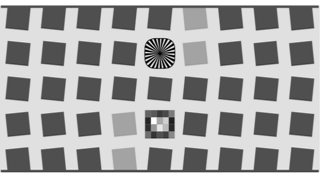 The standard SFRplus test chart consists of a 5x9 grid of squares, all but four of which have a 10:1 contrast ratio. The contrast ratio of the remaining four (one column off the center) is 2:1. A small 4x5 patch stepchart (densities in steps of 0.1 from 0.05 to 1.95) is located below the central square. The top and bottom rows of squares are bounded by bars for measuring distortion.
The chart can be purchased a chart from the Imatest store. It should be mounted on 32x40 or 40 x60 inch sheets of 1/2 inch (12.5 cm) thick foam board with spray adhesive or double-sided tape. 1/2 inch foam board stays flatter than standard 1/4 or 3/8 inch board.
Photograph the chart.
Frame the chart so that
- there is white space above and below the bars (used to measure distortion) at the top and bottom of the images. This space should be at least 0.5% and no more than 25% of the total image height. Ideally the white space should be 2-8% of the image height. The chart should be vertically centered, but this is not necessary for SFRplus to run successfully.
- The stepchart pattern is close to the horizontal center of the chart.
- The sides of the chart may extend beyond the image (as shown below) or be well within the image. The software is designed to accommodate a wide variety of framing and aspect ratios. Edges closest to the left and right boundaries will always be properly located. If the left and right sides of the chart are inside the image, there should be no interfering patterns in the image that could be mistaken for chart features— the chart should be surrounded with plain white or light gray.
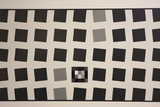
Well-framed SFRplus image
- The chart should be aligned correctly using techniques and tricks shown in The Imatest Test Lab. Moderate misalignment is tolerated by SFRplus: a tilt of 1-2 degrees, perspective distortion, etc., but every effort should be made to align the chart properly. Moderate barrel or pincushion distortion (<5% SMIA) is also well tolerated, but Fisheye lenses (with high, intentional barrel distortion) will probably fail.
If exposure compensation is available, you may want to use it to get a good exposure: typically by overexposing +1 f-stop.
Bad framing
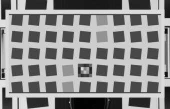
Interfering patterns near borders |
Good framing
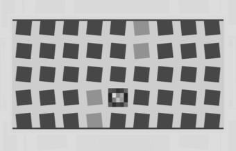
Same pattern; interfering patterns masked out |
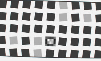
No white space above top distortion bar
|
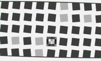
Some tilt, distortion tolerated |
Lighting
The chart below summarizes lighting considerations. The goal is even, glare-free illumination. Lighting angles between 30 and 45 degrees are ideal in most cases. At least two lights (one on each side) is recommended; four or six is better. Avoid lighting behind the camera, which can cause glare. Check for glare and lighting uniformity before you expose. A detailed description of the recommended lighting setup, which uses six high quality (CRI > 98) 4700K (near-daylight) 50W SoLux quartz-halogen lamps, can be found in The Imatest Test Lab. SoLux Task Lamps may also be used. The BK Precision 615 Light meter (Lux meter) is an outstanding low-cost instrument (about $100 USD) for measuring the intensity and uniformity of illumination.
Simplified lighting diagram
Distance
| Distance and field of view |
| The camera must be far enough from the chart so you are measuring the sharpness of your camera and lens, not the chart. But remember, |
It's the field of view, not the chart-to-camera distance, that counts.
|
| A rough rule of thumb: For an inkjet-printed chart the field of view should be at least |
22 inches (60 cm) for a 6-megapixel camera;
35 inches (90 cm) for a 16 megapixel camera. |
| Details below. For a high-quality photographically-printed chart (such as the charts from Applied Imaging) you can get quite a bit closer. |
|
A letter-sized (8.5x11 inch) chart printed on Premium Luster paper on the Epson 2200 (a high quality pigment-based inkjet photo printer) was analyzed for MTF using the 6.3 megapixel Canon EOS-10D. There was no change when the image field was at least 22 inches (56 cm) wide— twice the length of the chart. Performance fell off slowly for smaller fields.
Choose a camera-to-target distance that gives at least this image field width. The actual distance depends on the sensor size and the focal length of the lens. The minimum image field is illustrated on the right.
Cameras with more pixels, and hence higher potential resolution,
should
should have a larger image field width, hence printed chart width.
Distance/field width guidelines for high quality inkjet charts
(You can get closer with photographically-printed charts.) |
| The
camera-to-target
distance is not critical as long as it is greater than a reasonable
minimum. |
Sensor sizes |
Desig-
nation |
Diagonal
mm. |
Width
mm. |
Height
mm. |
| 1/3.6" |
5.0 |
4.0 |
3.0 |
| 1/3.2" |
5.68 |
4.54 |
3.42 |
| 1/3" |
6.0 |
4.8 |
3.6 |
| 1/2.7" |
6.59 |
5.27 |
3.96 |
| 1/2" |
8.0 |
6.4 |
4.8 |
| 1/1.8" |
8.93 |
7.18 |
5.32 |
| 2/3" |
11.0 |
8.8 |
6.6 |
| 1" |
16.0 |
12.8 |
9.6 |
| 4/3" |
22.5 |
18.0 |
13.5 |
| 35mm |
44.3 |
24.0 |
36.0 |
|
Image field
width (in inches) > 8.8 × sqrt(megapixels)
( > means "greater than.")
Image field
width (in
cm) > 22 × sqrt(megapixels)
— or —
There should
be no more
than 140 sensor pixels per inch of target or 55 sensor pixels per
centimeter
of the target.
— or —
The distance
to the target
should be at least 40X the focal length of the lens for 6-10 megapixel digital SLRs.
(25X
is the absolute minimum for 6 megapixel DSLRs; 40X leaves some margin.) For compact digital
cameras,
which have much smaller sensors, the distance should be at least 100X
the actual
focal length: the field of view is about the same as an SLR with
comparable
pixel count. The recommended distance is described in more detail in Chart
quality and distance, below. |
There is some confusion about lens focal lengths in compact digital cameras. They are often given as the "35mm-equivalent," which many photographers can relate to viewing angle. 35-105mm or 28-140mm are typical "35mm-equivalent" numbers, but they are not the true lens focal length, which is often omitted from the specs. What is given is the sensor size in 1/n inches, a confusing designation based on the outside diameter of long-obsolete vidicon tubes. It The table on the right relates the 1/n designation to the diagonal dimension of the sensor.
True focal length = "35mm-equivalent" × (diagonal mm.) / 44.3 |
Exposure |
|
Good exposure is important
for accurate SFRplus
results.
Neither the black nor the white regions of the chart should clip—
have substantial areas that reach pixel levels 0 or 255. The best way
to
ensure proper exposure is to use the histogram in your digital camera.
Blacks (the peaks on the left) should be above the minimum and whites
(the
peak(s) on the right) should be below the maximum. |
|
The above image (taken from the Canon File Viewer Utility) is close
to a perfect exposure. Some exposure compensation, typically around +1 f-stop, may be helpful.
| Tips
on photographing the chart |
| Distance
doesn't matter
as long as the target far enough from the camera so sharpness is
limited
by the camera and lens, not
by the target. For a target printed on the Epson 2200 printer, a
distance
that gives at least a 24 inch (horizontal) field of view seems to be
sufficient. |
| The target
should be evenly
lit and free of glare. |
| White
balance should be
approximately neutral. |
| Use a
sturdy tripod and
a cable release. If possible, use the mirror lock. You can use Imatest
SFR to find the difference made by a good tripod or mirror lock— to
sharpen
your technique, literally ( pun intended ). |
| Be sure to
expose the image
so detail is maintained in both light and dark areas. Neither should be
blocked (clipped). Use your camera's histogram. If more than 0.5% of
the
pixels are at levels 0 or 255, Imatest SFR will assume that clipping
has
taken place and issue a warning message. This has no effect on the
calculations—
it's just a warning that accuracy may be compromised. |
| Be sure
the camera is correctly
focused on the chart. |
| Place
slanted-edge images
near the corners of the field as well as near the center. |
| You may
find it instructive
to photograph the slanted edge target along with a target from Lens
testing, but there's no need to do so. |
|
Save the image as a RAW file or maximum quality JPEG. If you are
using
a RAW converter, convert to JPEG (maximum quality), TIFF (without LZW
compression,
which is not supported), or PNG. If you are using film, develop and
scan
it. The file name should be descriptive and should indicate the
parameters
you are testing. Use dashes and underscores ( - and _ ), but avoid
spaces.
(Spaces work with Imatest, but they can be troublesome in DOS command
lines
and web pages.) An example would be Canon_EOS10D_70-200f4L_100mm_f8_ctr.jpg.
You are now ready to run
Imatest
SFRplus.
Using SFRplus Part 2
Running Imatest SFRplus
Running
SFRplus
Imatest SFRplus performs highly automated measurements of several key image quality factors using a specially-designed test chart. This document shows how to run SFRplus inside Rescharts and how to save settings for automated runs. Part 1 introduced SFRplus and explained how to obtain and photograph the chart. Part 3 illustrates the results.
Open Imatest by double-clicking the Imatest icon on
- the Desktop,
- the Windows Start menu,
- the Imatest folder (typically C:\Program files\Imatest in English language installations).
After several seconds, the Imatest main window opens. Then click on Rescharts or SFRplus on the upper left.
SFRplus operates in two modes.
Use Rescharts to initiate an interactive/setup SFRplus run. This allows you to examine detailed results interactively to to save settings for the highly automated SFRplus runs. Rescharts should be run at least once prior to the first SFRplus run. |
|
 Rescharts SFRplus
Selecting file(s)
The portion of the Rescharts window used for opening files is shown on the right. You can open a file by clicking on Read image file if the correct chart type is displayed, or by selecting a Chart type. One or more files may be selected, as shown below. If you select multiple files, they will be combined (averaged), and you'll be given the option of saving the combined file.
If the folder contains meaningless camera-generated file names such as IMG_3734.jpg, IMG_3735.jpg, etc., you can change them to meaningful names that include focal length, aperture, etc., with the View/Rename Files utility, which takes advantage of EXIF data stored in each file.
The folder saved from the previous run appears in the Look in: box on the top. You are free to change it. You can open a single file by simply double-clicking on it. You can select multiple files for combined runs (in Imatest Master) by the usual Windows techniques: control-click to add a file; shift-click to select a block of files. Then click Open. Three image files for the Canon 17-40mm L lens are highlighted. Large files can take several seconds to load. Batch (sequential) runs are not supported in Rescharts
File selection
| Multiple file selection Several files can be selected in Imatest Master using standard Windows techniques (shift-click or control-click). The files are combined to reduce noise and (in some instances) observe the effects of camera shake or image stabilization. The multi-image dialog box gives you the option of saving the combined file, which will have the same name as the first selected file with _comb_n appended, where n is the number of files combined. Batch mode, which allows several files to be analyzed in sequence, is not supported by Rescharts |
|
| RAW files Starting with Imatest Master 2.7 (February 2008) Imatest SFR can analyze Bayer raw files: standard files (TIFF, etc.) that contain undemosaiced data. RAW files are not very useful for measuring MTF because the pixel spacing in each image planes is twice that of the image as a whole; hence MTF is lower than for demosaiced files. But Chromatic aberration can be severely distorted by demosaicing, and is best measured in Bayer RAW files (and corrected during RAW conversion). Details of RAW files can be found here. |
SFRplus settings windows
SFRplus parameters & setup window
Shortly after the file (or files) have been selected the SFRplus parameters & setup window, shown below, appears. This window allows you to select groups of regions (ROIs) for analysis, shown as violet rectangles. It also lets you select the size of the regions, whether to analyze vertical or horizontal edges, and change several additional settings. Pressing the Settings & options button on the left opens the SFRplus Settings & options window, which allows you to select additional settings that affect the calculations, display, and output (for automated SFRplus runs). The light yellow-orange rectangles are for calculating the Color/lightness uniformity profiles.
SFRplus parameters & setup window; 9 regions selected for analysis
| SFRplus parameters & setup window controls Settings |
| Settings area |
| Gamma |
Assumed Gamma (contrast) of the chart. Has a small effect on the MTF results. Default is 0.5. |
| Channel |
Select channel to analyze: R, G, B, Y, R-only, G-only, B-only, Y-only. (Y is Luminance channel). Use one channel only where other channels are dark and may not contain valid data. |
Chart contrast
(for gamma calc.) |
Chart contrast-- for the contrasty squares (i.e., most of them). Used to estimate gamma from the image. |
| Use for MTF |
(Checkbox, normally unchecked) When checked, use the gamma derived from the chart for the MTF calculation. This may result in a small improvement in accuracy. |
| Display options |
Open the SFRplus settings & options window, shown below. |
| ROI selection area |
Region (center, etc)
(Selects which regions
to locate. Actual ROIs
are located automatically) |
Select the regions (ROIs) to analyze. Choices below. The number of regions is in parentheses. This is a particularly important setting. We encourage users to become familiar with each of the settings below.
Center (1).
Center & corners (5).
Center, corners, part-way (9) (Part-way is on diagonal between center & corners). This setting is often a good compromise between speed and detail.
Center, L, R, T, B (9).
Center, corners, part-way, L, R, T, B (13).
Maximum regions (23) (edges on a 5x5 grid, omitting the squares above and below the center). Highly detailed results. |
| Vertical, Horizontal edges |
Chooses between Vertical and Horizontal edges. Usually Vertical, but Horizontal is useful on occasion.. |
| ROI size |
Slider that determines the size of the ROI. Use the largest value that keeps a save distance from edges of squares and top and bottom bars. May have to be reduced where distortion is severe. |
ROI width
(below ROI size slider) |
Width of ROI selection. Normal width for the standard rectangular ROI. Choose Wider or Widest for enhanced noise analysis. |
| Other controls |
| Title |
Title. Defaults to file name. You can add a description. |
| Help |
Open this web page in a web browser. |
| Image setting |
Selects image channel for display: Original (RGB) image, Red, Green, or Blue channels |
| Save settings |
Save settings (for use in auto SFRplus), but do not continue with run. |
| OK |
Save settings and continue with run: Calculate results for all selected region. You will be able to view results interactively. |
| Cancel |
Cancel run; do not save settings |
After you've finished making settings, click OK to save settings and continue with the run. You can Click Save settings to save the settings without continuing.
SFRplus settings & options window
The SFRplus settings & options window, shown below, opens when Display options in the parameters & setup window is pressed. The settings are read from the rescharts.ini file, and saved to both imatest.ini and rescharts.ini when OK is pressed. Settings are similar to the settings in the SFR input dialog box.
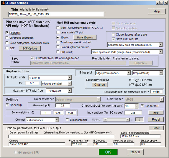
SFRplus settings & options window
This window is divided into sections: Title and Help on top, then Plot and save, Display options, Settings, Optional parameters, and finally, OK or Cancel.
Title
defaults
to the input file name. You may leave it unchanged, replace
it, or add descriptive information for the camera, lens, converter settings, etc.— as
you please.
Help opens a browser window containing a web page describing the module. The browser window sometimes opens behind other windows; you may need to check if it doesn't pop right up.
Plot and save (for SFRplus Master auto/API only; NOT for Rescharts).
This area selects figures to plot and save as well as a number of data save settings. It only applies to the automatic version of SFRplus in Imatest Master — it is not for Rescharts.
The leftmost checkboxes in this section select figures to plot and save. Note that all plotted figures are saved. Saved figures, CSV, and XML files are given names that consist of a root file name (which defaults to the image file name) with a suffix added. Examples:
Canon_17-40_24_f8_C1_1409_YR7_cpp.png
Canon_17-40_24_f8_C1_1409_YR7_MTF.csv
Close figures after save should be checked if a large number of figures is to be displayed. It prevents a buildup of figures, which can slow processing.
A CSV summary file is saved for all runs. An XML file is saved if Save XML results is checked.
You can select either Save CSV files for individual ROIs or Save summary CSV file only (the summary file is always saved).
Save folder determines where to store results. It can be set either to subfolder Results of the image folder or to a folder of your choice.
|
Display options (to the right of Plot) contains settings that affect the plot display.
MTF plots (individual and summary) selects the spatial frequency scale for MTF plots for for the summary plot. Cycles/pixel (C/P), Cycles/mm (lp/mm), Cycles/inch (lp/in), Line Widths per Picture Height (LW/PH), and Line Pairs per Picture Height (LP/PH) are the choices. (Note that one cycle is the same as one line pair or two line widths.) If you select Cycles
per inch or Cycles/mm,
you must enter a number for the pixel size— either in pixels
per inch, pixels
per mm, or microns
per pixel. For more detail on pixel size, see the box below.
Maximum MTF plot frequency selects the maximum display frequency for MTF plots. The default is 2x Nyquist (1 cycle/pixel). This works well for high quality digital cameras, not for imaging systems where the edge is spread over several pixels. In such cases, a lower maximum frequency produces a more readable plot. 1x Nyquist (0.5 cycle/pixel), 0.5x Nyquist (0.25 cycle/pixel), and 0.2x Nyquist (0.1 cycle/pixel) are available.
Chart contrast For a medium or low contrast charts (contrast <= 40; not recommended with the old ISO 12233 chart), you can enter the chart contrast (or Off). If the ROI is large enough, the actual (measured) gamma will be calculated and displayed along with the contrast factor (the chart contrast multiplier = measured gamma/nominal gamma, where nominal gamma is entered in the Settings area, described below). If the Use for MTF box just to the right is checked, this value will be used in the MTF calculation, which may result in a modest improvement in accuracy.
Secondary readout controls the secondary readout display in MTF plots. The primary readout is MTF50 (the half-contrast spatial frequency); the secondary readout has several options. It defaults to MTF30 (the spatial frequency where MTF is 30%).
Clicking Change opens the window shown on the right. Secondary readout settings are saved between runs. Choices:
- The upper radio button (MTF) selects MTFnn, the spatial frequency where MTF is nn% of its low frequency value.
- The middle radio button selects MTFnnP, the spatial frequency where MTF is nn% of its peak value: useful with strongly oversharpened edges.
- The lower radio button (MTF @ ) selects MTF @ nn units, where nn is a spatial frequency in units of Cycles/pixel, LP/mm, or LP/in. If you select this button, the pixel spacing should be specified in the Cycles per... line in the Plot section of the input dialog box, shown above. A reminder message is displayed if the pixel spacing has been omitted.
Edge plot selects the contents of the upper (edge) plot. The edge can be cropped (default) or the entire edge can be displayed. Three displays are available.
- Edge profile (linear) is the edge profile with gamma-encoding removed. The values in this plot are proportional to light intensity. This is the default display.
- Line spread function (LSF) is the derivative of the linear edge profile. MTF is the fast fourier transform (FFT) of the LSF. When LSF is selected, LSF variance (σ2), which is proportional to the DxO blur unit, is displayed.
- Edge pixel profile is proportional to the edge profile in pixels, which includes the effects of gamma encoding.
|
Settings affect the calculations as well as the display.
Gamma is
used to linearize the input data, i.e., to remove the gamma encoding applied in the camera or RAW converter. It defaults to 0.5
= 1/2, which is typical of digital cameras, but is affected by camera or RAW converter contrast settings. It should be set to 0.45 when RAW images are read into Imatest (to be converted by dcraw), but there is little loss in accuracy if it is left at 0.5. If is is set to less than 0.3 or greater than 0.8, the background will be changed to pink to indicate an unusual (possibly erroneous) selection.
Since SFR sharpness measurements are moderately sensitive to the
Gamma setting (a 10% error in gamma results in a 2.5% error in MTF50 for a normal contrast target), it's a good idea to run Colorcheck or Stepchart to determine the correct value of Gamma. A nominal value of gamma should be entered, even if the value of gamma derived from the chart (described above) is used to calculate MTF.
| Gamma |
Gamma is the exponent of the equation that relates image pixel level to luminance. For a monitor or print,
Output luminance = (pixel level)gamma_display
When the raw output of the image sensor, which is linear, is converted to image file pixels for a standard color space, the approximate inverse of the above operation is applied.
pixel level = (RAW pixel level)gamma_camera ~= exposuregamma_camera
The total system gamma is gamma_display * gamma_camera. Standard values of display gamma are 1.8 for older color spaces used in the Macintosh and 2.2 for color spaces used in Windows, such as sRGB (the default) and Adobe RGB (1998).
In practice, gamma is equivalent to contrast. More detail on gamma can be found in SFR Instructions, part 2. |
|
Channel is normally left at it's default value of Y for the luminance channel,
where Y = 0.3*R + 0.59*G + 0.11*B.
In rare instances the R, G, and B color channels might be of interest.
Reset restores the settings in Options and Settings to their default values. |
Additional parameters
(all optional) for Excel .CSV output contains a detailed description of the camera, lens, and test conditions. EXIF data
is entered, if available, but can be overridden by manual settings. Description & settings is particularly useful for annotating the test system (it is displayed in MTF Compare).These settings are optional but can be useful when several
tests are run for different lenses, focal lengths, apertures, or other
settings. The settings are displayed next to the MTF plots. They are saved and reused in subsequent runs for files with the same pixel dimensions. If EXIF data is available (currently, only in JPEG files) it overrides the saved settings. The Reset button clears all entries. |
ISO standard SFR If this checkbox is checked, SFR calculations are performed according to the ISO 12233 standard, and the y-axis is labeled SFR (MTF) (ISO standard). This method is slightly less accurate than the normal Imatest calculation, which incorporates a number of refinements, including a better edge detection algorithm and a second-order polynomial fit to the average edge for a more accurate estimate of SFR in the presence of lens distortion. This box is normally left unchecked; it should only be used for comparing normal Imatest calculations to the ISO standard. The difference is typically very small.
When entries are complete, click OK to return control to the SFRplus settings & options window.
When all entries are complete, click either Save settings, OK, or Cancel. Save settings saves the settings for use in automated SFRplus runs, which can be initiated from the SFRplus button in the main Imatest window. OK saves the settings then calculates results for interactive viewing. A sequence of Calculating...
boxes appear to let you know how calculations are proceeding. When calculations are complete, results are displayed interactively in the Rescharts window, as shown below.
Warnings
A Clipping warning is issued if more than 0.5% of the pixels are clipped (saturated), i.e., if dark pixels reach level 0 or light pixels reach the maximum level (255 for bit depth = 8). This warning is emphasized if more than 5% of the pixels are clipped. Clipping reduces the accuracy of SFR results. It makes measured sharpness better than reality. |
|
The percentage of clipped pixels is not a reliable index of the severity of clipping or of the measurement error. For example, it is possible to just barely clip a large portion of the image with little loss of accuracy. The plot on the right illustrates relatively severe clipping, indicated by the sharp "shoulder" on the black line (the edge without standardized sharpening). The sharp corner makes the MTF look better than reality. The absence of a sharp corner may indicate that there is little MTF error. |
Clipping warnings |
Clipping can usually be avoided with a correct exposure-- neither too dark nor light. A low contrast target is recommended for reducing the likelihood of clipping: it increases exposure latitude and reduces the sensitivity of the MTF results to errors in estimating gamma.
SFRplus summary
- SFRplus analyzes images of the SFRplus test chart, framed so that there is white space above and below the horizontal bars in the chart, i.e., so neither bar runs off the image. The bars may, however, run off the sides of the image. The white space should be between 0.5% and 25% of the image height. There should be few or no interfering patterns (bars, etc.) outside the image of the chart itself.
- Lighting should be even and glare-free. Lighting and alignment recommendations are given in The Imatest test lab.
- The first time SFRplus is run, it should be run through Rescharts. This allows
- parameters to be adjusted and saved for later use in the automatic version of SFRplus, which is opened with the SFRplus button in the Imatest main window.
- results (listed above) to be examined interactively in the Rescharts window.
- The SFRplus button on the main Imatest window runs SFRplus in full automatic mode using settings saved from the most Rescharts run.
Next: Using SFRplus Part 3: Results
Pixel size
Pixel size has an important relationship to image quality. For very small pixels, noise, dynamic range and low light performance suffer. Pixel size is rarely given in spec sheets: it usually takes some math to find it. If the sensor type and the number of horizontal and vertical pixels (H and V) are available, you can find pixel size from the table on the right and the following equations.
pixel size in mm = (diagonal in mm) / sqrt(H2 + V2)
pixel size in microns = 1000 (diagonal in mm) / sqrt(H2 + V2)
Pixel size in microns (microns per pixel) can be entered directly into the SFR input dialog box. Example, the cute little 5 megapixel Panasonic Lumix DMC-TZ1 has a 1/2.5 inch sensor and a maximum resolution of 2560x1980 pixels. Guessing that the diagonal is 7 mm, pixel size is 2.1875 (rounded, 2.2) microns.You can find detailed sensor specifications in pages from Sony, Panasonic, and Kodak. |
Sensor
Designation
(Type) |
Diagonal
mm. |
Width
mm. |
Height
mm. |
| 1/4" |
4.5 |
|
|
| 1/3.6" |
5.0 |
4.0 |
3.0 |
| 1/3.2" |
5.68 |
4.54 |
3.42 |
| 1/3" |
6.0 |
4.8 |
3.6 |
| 1/2.7" |
6.59 |
5.27 |
3.96 |
| 1/2.5" |
6.9 - 7.2 |
|
|
| 1/2" |
8.0 |
6.4 |
4.8 |
| 1/1.8" |
8.93 - 9.1 |
7.18 |
5.32 |
| 2/3" |
11.0 |
8.8 |
6.6 |
| 1" |
16.0 |
12.8 |
9.6 |
| 4/3" |
22.5 |
18.0 |
13.5 |
| 35mm |
44.3 |
24.0 |
36.0 |
|
Using SFRplus Part 3
Imatest SFRplus results
Imatest SFRplus performs highly automated measurements of several key image quality factors using a specially-designed test chart. Unlike other modules, the user never has to manually select Regions of Interest (ROIs). Image quality factors include
This document illustrates SFRplus results. Part 1 introduced SFRplus and explained how to obtain and photograph the chart. Part 2 showed how to run SFRplus inside Rescharts and how to save settings for automated runs.
SFRplus results
When calculations are complete, results are displayed in the Rescharts window, which allows a number of displays to be selected. A general description can be found on Using Rescharts.
Multi-ROI summary display
SFRplus results in Rescharts window: Multiple region (ROI) summary
The multi-ROI summary results shown in the Rescharts window (above) is the best summary of SFRplus results, but it is just one of several available displays. It is described in detail in Multiple ROI (Region of Interest) plot. The upper left contains the image in muted gray tones. The selected regions are surrounded by red rectangles and displayed with full contrast. Four results boxes are displayed next to each region. There is a legend below the image. The table below explains the contents in more detail.
| N: Ctr-corner distance % |
Region number (N) and distance from the center as a percentage of center-to-corner distance |
| MTF50 LW/PH or cycles/pxl |
MTF50 in units specified in the MTF plots entry in Display options in the SFRplus settings and options window. |
| MTF20 LW/PH or cycles/pxl |
MTF20 in the same units as MTF50. May be replaced by the secondary readout in an upcoming release. |
| Chrom Aberration (pxl area) |
Chromatic Aberration in pixel area. % of center-to-corner distance may be an option in a future release. See Chromatic Aberration and Chromatic Aberration ... plots. |
Distortion statistics are shown in the lower left. SMIA TV distortion is the simplest overall measure of distortion. k1 (the third order distortion coefficient) and the Picture Window Pro arctangent/tangent coefficients are discussed on the page on Distortion.
The upper right contains a display of Weighted MTF50 results that covers the small image visible in the other plots. The weighted sum has weights of 1 for ROIs in the central region (inside the inner dotted circle), 0.75 for the middle region (between the two dotted circles), and 0.25 for the outer region (outside the outer dotted circle). The results are independent of the number of ROIs in each region.
Plot settings area
A small number of options are available in the Plot settings area, on the lower right, below the Display box (fewer than for other Rescharts modules).
All displays contain the dropdown menu for selecting the primary channel to analyze. If R, G, B, or Y (Luminance) is selected, all channels are analyzed, but the selected channel is emphasized. There is also an option to analyze any of the channels alone— useful where one of the secondary channels is dark and may cause a run to crash. Luminance (Y) is shown above. If it is changed, results are recalculated.
All displays except Multi-ROI summary and Tonal response & gamma allow you to select the ROI for viewing results.
The Edge and MTF display has a dropdown window for selecting the maximum MTF display frequency: 2x Nyquist (the default), Nyquist, 0.5x Nyquist, and 0.2x Nyquist.
Edge and MTF display
Edge and MTF display in Rescharts window
This display is identical to the SFR Edge and MTF display. MTF is explained in Sharpness: What is it and how is it measured? The edge (or line spread function) is plotted on the top and the MTF is plotted on the bottom. There are a number of readouts, including 10-90% rise distance, MTF50, MTF50P (the spatial frequency where MTF is 50% of the peak value; differing from MTF50 only for oversharpened pulses), the secondary readout (MTF20 in this case), and the MTF at the Nyquist frequency (0.5 cycles/pixel).
An important (and optional) readout in the upper plot is
- The Chart contrast (entered in the Display options section of the SFRplus settings & options window),
- The Contrast factor: the ratio between the chart contrast derived from the pixel ratio and the input value of gamma (0.5 in the above display),
- Gamma (from chart): a measurement of gamma derived from the chart pixel levels and the Chart contrast (an input value, as described above). Gamma has a relatively small effect on the MTF measurement, especially for moderate to low contrast targets (10:1 or under).
Chromatic Aberration
Lateral Chromatic Aberration (LCA), also known as "color
fringing,"
is most visible on tangential boundaries near the edges of the image. Much of the plot is grayed out if the selected region (ROI) is too close to the center (less than 30% of the distance to the corner) to accurately measure CA.
The area between the highest and lowest of the edge curves (shown for the R, G, B, and Y (luminance) channels) is a perceptual measurement of LCA. It has units of pixels because the curves are normalized to an amplitude of 1 and the x-direction (normal to the edge) is in units of pixels. It is displayed as a magenta curve. |
Lateral Chromatic Aberration |
Perceptual LCA is also expressed as percentage of the distance from center to corner, which tends to be more reflective of system performance: less sensitive to location and pixel count than the pixel measurement. Values under 0.04% of the distance from the center are insignificant; LCA over 0.15%
can be quite visible and serious.
Information for correction LCA (R-G and B-G crossing distances) is also given in units of % (center-to-corner) and pixels. LCA can be corrected most effectively before demosaicing. Results are explained in Chromatic Aberration ... plot. |
SQF (Subjective Quality Factor)
SQF is a perceptual measurement of the sharpness of a display (monitor image or print). MTF, by comparison is device sharpness (not perceptual sharpness). SQF includes the effects of the human visual system's Contrast Sensitivity Function (CSF), print (or display) size, and viewing distance (which is assumed to be proportional to print height, by default).
See Introduction to SQF for more detail. |
SQF (Subjective Quality Factor) |
Tonal response & gamma
This display is derived from the 4x5 stepchart pattern, located just below the central square of the SFRplus test chart. It resembles the third figure in Stepchart. The upper plot shows the tonal response for all colors. The lower plot shows instantaneous gamma— the slope (derivative) of tonal response. The value of gamma may differ slightly from the values in the Edge response and MTF display because it's calculated differently-- based on the average slope of the light to middle tone squares of the stepchart. |
Tonal response & gamma |
Histograms and noise analysis
This display contains histograms of pixel levels for individual ROIs (original on top and linearized using input gamma on bottom). The black (background) histogram contains pixel levels for the entire ROI. The red histogram is for the right (dark) region, away from the transition, used in the noise statistics calculation. The cyan histogram is for the left (light) region. Sharpening may cause extra bumps to appear in the black histogram. A detailed level and noise analysis is displayed below the image.
| Dark, light levels |
Original pixel levels normalized to 1 and linearized levels, also normalized to 1 |
| Estimated chart contrast (for gamma = ...) |
The correct chart contrast must be entered in SFRplus parameters & setup window. |
| Noise (dark, light, mean; norml pixels %) |
RMS noise expressed in pixels, normalized to 100% (for 255 in 8-bit files) |
| S/N (...; norml pixels) |
Signal/Noise, where signal is mean pixel level of ROI at a distance from the transition. |
| Noise (...; linearized %) |
Noise, linearized using gamma (input); normalized to 100% |
| S/N (...; linearized) |
Signal/Noise, linearized |
|
Histograms and noise stats |
Noise calculations are made in portions of the ROIs (Regions of Interest) away from the transitions. They are facilitated by selecting wide ROIs. The noise spectrum on the lower right contains qualitative information about noise visibility and software noise reduction, which generally reduces high frequency noise below 0.5, typical of demosaicing alone. The region on the right is shown in red; left is shown in cyan. See also Noise. |
Color & lightness uniformity profiles
This display is similar in some respects to the profile plots in Light Falloff. It consists of profiles of the light areas (average values of rectangles between squares). Left-to-right profiles of the top, middle, and bottom of the image are shown on the left side of the display, and top-to-bottom profiles at the left, center, and right of the image are shown on the right. The following display options are available.
R, G, B, and Y unnormalized (max = 1)
R, G, B, and Y normalized (max = 1)
R, G, B, and Y unnormalized (max = 255)
R/G (Red) and B/G (Blue) unnormalized
R/G (Red) and B/G (Blue) normalized (max = 1)
Delta-L* (gray), a* (R), b* (B), chroma c* (G)
For best results with this display, you should make every effort to illuminate the target uniformly using techniques in The Imatest Test Lab. Brightness-related results (R, G, B, Y, and Delta-L*) cannot be measured as accurately as with Light Falloff, where the recommended technique calls for a clear uniform image field photographed through opal diffusing glass. But they can still be useful. The color ratios (R/G, etc.) can be especially useful for diagnosing uneven color response. |
Uniformity profiles |
Image display
This display allows several aspects of the image to be viewed in detail. It shows the selected regions for MTF/noise analysis (violet rectangles) as well as the yellow rectangles used for generating the uniformity profiles. Display options include
(original) Color image
Red, Green, or Blue channel
Color image with HSV satuartion boosted 4X or 10X.
|
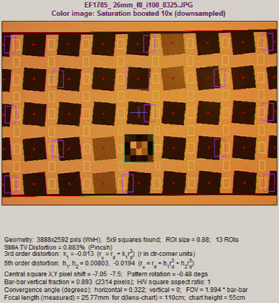
Image (shown with exaggerated saturation) |
Summary & EXIF data
This plot contains summary results for individual ROIs and EXIF data (metadata that describes camera and lens settings). When first installed, Imatest reads EXIF data from JPEG files only. Enhanced EXIF support requires a special download of ExifTool, described here. |
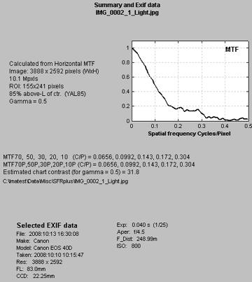
Summary & EXIF data |
SFRplus summary
- SFRplus analyzes images of the SFRplus test chart, framed so that there is white space above and below the horizontal bars in the chart, i.e., the bars must not run off the top or bottom of the image. They may, however, run off the sides of the image. The white space should be between 0.5% and 25% of the image height. There should be few or no interfering patterns (bars, etc.) outside the image of the chart itself.
- Lighting should be even and glare-free. Lighting and alignment recommendations are given in Building a test lab.
- The first time SFRplus is run, it should be run through Rescharts. This allows
- parameters to be adjusted and saved for later use in the automatic version of SFRplus, which is opened with the SFRplus button in the Imatest main window.
- results (listed above) to be examined interactively in the Rescharts window.
Result file
names— The roots of the file names are
the same as the image file name. The channel (Y, R, G, or B) is included
in the file name. If a Region of Interest has been selected from a complete
digital camera image, information about the location of the ROI is included
in the file name following the channel. For example, if the center of the
ROI is above-right of the image, 20% of the distance from the center to
the corner, the characters AR20 are included in the file name.
Output files
for filename.jpg (Y-channel)
(default location:
subfolder Results)
| Figures
(.PNG image files) |
| filename_YA17_cpp.png |
Plot with x-axis in cycles/pixel (c/p), Y-channel,17% of the way to
the corner above the center of the uncropped image. |
| filename_YA17_lwph.png |
Plot with x-axis in Line Widths per Picture Height (LW/PH). |
| filename_YA17_ca.png |
Plot of Chromatic Aberration, with noise statistics and Shannon information
capacity. |
| Excel
.CSV (ASCII text files that can be opened in Excel) |
| CSV output files are explained in detail below. Click link for detail on individual file. |
| filename_YA17_MTF.csv |
Excel .CSV file of MTF results for this run. All channels (R, G, B, and Y (luminance) ) are displayed.The first row has the
headers: cy/pxl, LW/PH, MTF(nchan), MTF(corr), MTF(R), MTF(G), MTF(B), MTF(Y), where nchan is the selected channel. The remaining lines contain the
data. Can easily be plotted or combined with data from other files. |
| filename_Y_multi.csv |
Excel .CSV file of summary results for a multiple ROI run. |
| filename_Y_sfrbatch.csv |
Excel .CSF file combining the results of batch runs (several files) with multiple ROIs. Particularly useful for generating easily-readable Excel plots. |
Excel
.CSV (Comma-Separated Variables) and XML output
Imatest SFR creates or updates output files for use
with Microsoft Excel. The files are in CSV (Comma-Separated Variable) format,
and are written to the Results subfolder by default. .CSV files are ASCII text files
that look pretty ugly when viewed in a text editor:
File
,Date/time
,PH,Ch,H/V,10-90U,10-90C,Over-,Over-,MTF50U,MTF50C,MTF,Camera,Lens,FL,f-stop,Loc,Misc.
,,,,,/PH,/PH,shoot%,sharp%,LW/PH,LW/PH,Nyq,,,(mm),,,settings
canon_eos10d_sfr.jpg,2004-03-19
22:21:34, 2048,Y,H, 1422, 1447, 19.5, -0.7, 1334, 1340,0.154,,,,,
canon_g5_sfr.jpg,2004-03-19
22:24:30, 1955,Y,H, 1973, 1301, 48.0, 21.3, 1488, 1359,0.268,Canon G5,—,14,5.6,ctr,
sigma_sd9_sfr.jpg,2004-03-19
22:27:55, 1504,Y,H, 1432, 1676, 2.4, -7.7, 1479, 1479,0.494,,,,,
sigma_sd10_sfr.jpg,2004-03-19
22:28:32, 1504,Y,H, 1563, 1628, 11.9, -2.0, 1586, 1587,0.554,,,,, |
But they look fine when opened in
Excel.
.CSV files can be edited with standard
text editors, but it makes more sense
to edit them in Excel, where columns as well as rows can be selected, moved, and/or
deleted. Some fields are truncated in the above display, and Date/time
is displayed as a sequence of pound signs (#####...).
The format can be changed by dragging the boundaries between cells on
the header row (A, B, C, ...) and by selecting the first two rows and setting
the text to Bold. This makes the output look better. The modified
file can be saved with formatting as an Excel Worksheet (XLS) file. This,
of course, is just the beginning.
It's easy to customize the Excel spreadsheet to your liking.
For example, suppose you want to make a concise chart. You can delete Date/time
(Row B; useful when you're testing but not so interesting later) and Channel
(all Y = luminance). You can add a blank line under the title, then you
can select the data (rows A4 through J7 in the image below) and sort on
any value you choose. Corrected MTF50 (column I) has been sorted in descending
order. Modified worksheets should be saved in XLS format, which maintains
formatting.
There are no limits. With moderate skill you can plot columns of results. I've said enough. ( I'm not an
Excel expert! )
Summary .CSV and XML
files for MTF and other data
An optional .CSV (comma-separated variable) output file contains results for MTF and other data. Its name
is [root name]_[channel location]_MTF.csv, where channel is (R, G, B, or Y) and the location BL75 means below-left, 75% of the distance to the corner (from the center). An example is Canon_17-40_24_f4_C1_1408_YBL75_MTF.csv. Excerpts are shown below, opened in Excel.
A portion of the summary CSV file, opened in Excel
The format is as follows:
| Line 1 |
Imatest, release (1.n.x), version (Light, Pro, Eval), module (SFR, SFR multi-ROI, Colorcheck, Stepchart, etc.). |
| File |
File name (title). |
| Run date |
mm/dd/yyyy hh:mm of run. |
| (blank line) |
| Tables |
Separated by blank lines if more than one. Two tables are produced. |
| The first table contains MTF. The columns are Spatial frequency in Cy/mm, LW/PH, MTF (selected channel), MTF (Red), MTF (Green), MTF (Blue), MTF (Luminance = Y). (...) represent rows omitted for brevity. |
| The second table contains the edge. Columns are x (location in pixels), Red edge, Green edge, Blue edge, Luminance (Y) edge, and Chromatic Aberration (the difference between the maximum and minimum). |
| (blank line) |
| Additional data |
The first entry is the name of the data; the second (and additional) entries contain the value. Names are generally self-explanatory (similar to the figures). |
| (blank line) |
| EXIF data |
Displayed if available. EXIF data is image file metadata that contains important camera, lens, and exposure settings. By default, Imatest uses a small program, jhead.exe, which works only with JPEG files, to read EXIF data. To read detailed EXIF data from all image file formats, we recommend downloading, installing, and selecting Phil Harvey's ExifTool, as described here. |
This format is similar for all modules. Data is largely self-explanatory. Enhancements to .CSV files will be listed in the Change Log.
The optional XML output file contains results similar to the .CSV file. Its contents are largely self-explanatory. It is stored in [root name].xml. XML output will be used for extensions to Imatest, such as databases, to be written by Imatest and third parties. Contact us if you have questions or suggestions.
An optional .CSV file is also produced for multiple ROI runs. Its name is [root name]_multi.csv.
MTF Compare
Compare MTFs of different cameras and lenses
Introduction to MTF Compare
MTF Compare, a module of Imatest Master, is a post-processor for comparing the MTFs of different cameras, lenses, and imaging systems after they have been analyzed by SFR or Rescharts Slanted-edge SFR and had results saved in CSV files. Comparisons are displayed as quotients of MTFs, i.e., transfer functions. For two imaging systems A and B, MTF Compare
- plots MTF(A)/MTF(B) or MTF(B)/MTF(A) along with MTF(A) and MTB(B) (shown as faint lines below). Details depend on the Display setting.
- Displays ratios or values of MTFnn (spatial frequencies where MTF is nn% of the low frequency value) and MTFnnP (spatial frequencies where MTF is nn% of the peak value) for nn = 70, 50, 30, 20, and 10.
These comparisons contain more detail than simple comparisons of MTF50 or other summary results (MTF20, etc.). As with all Imatest modules, a great many display options are available.
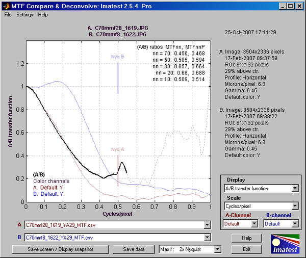
MTF comparison of Canon 24-70mm f/2.8L, 70mm, high contrast edge near center
A. f/2.8 (pale brown), B. f/8 (pale blue)
MTF Compare opens some intriguing new possibilities for Imatest. By using an autocollimator to project a slanted-edge pattern on a sensor, sensor MTF can be measured in isolation— without the effects of a lens. If the same sensor is then measured with a lens, MTF Compare can be used to factor out the sensor MTF (as well as that of the signal processing) so the MTF of the lens itself can be measured. This is done by dividing the system MTF by the sensor-only MTF. We are working with well-known autocollimator manufacturer to create an integrated turnkey solution. Stay tuned...
This plot above compares the results of two SFR runs for the same lens and focal length at two different apertures (f/2.8 and f/8) using the same high contrast edge above the center of the Applied Image QA-77 test chart. The SFR run for f/8 (B, above) is shown greatly reduced on the right. The A/B transfer function (MTF(A)/MTF(B)) is shown as a solid bold black line —— up to the lowest frequency where the denominator (MTF(B)) drops below 0.04. Results above this frequency are unreliable due to noise; hence they are shown as a dashed thin gray line - - - -.
In the MTF Compare figure (above) the input file names (csv files saved from SFR runs) are shown in the A. and B. boxes below the plot. The corresponding image file names are shown above the plot. The A and B Nyquist frequencies are shown as short, faint brown and blue lines. Important input data is summarized on the right.
Since the input to MTF Compare is saved SFR output, and since no Imatest output can be saved in evaluation mode, MTF Compare is not practical for running in evaluation mode. |
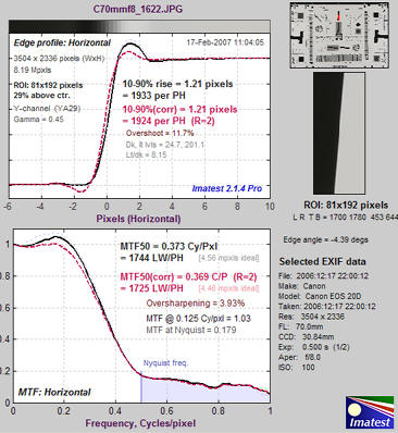 |
Instructions
Getting started
MTF Compare is a post-processor for Imatest SFR and Rescharts Slanted-edge SFR that uses SFR's Excel-readable CSV output files. In order to compare MTFs, these CSV output files must be saved in SFR runs. To do so, make sure Excel .CSV detailed results is checked in the SFR Save dialog box, shown on the right. You may, if you wish, change the Results directory and root file name from their defaults to make them easier to identify and retrieve. Then press Yes on the bottom. |
 |
The illustration below is similar to the one near the top of the page, except that it is based on the low-contrast edge closer to the center of the image of the QA-77 chart, which has much less in-camera sharpening than the high-contrast edge and the maximum display frequency is 0.5 cycles/pixel. The EOS-20D, like most digital cameras, has significant nonlinear signal processing, i.e., strong sharpening takes place in the vicinity of high contrast features, but little, if any, sharpening takes place in their absence— i.e., sharpening is not applied uniformly throughout the image. But even though the MTFs are much lower than the MTFs of the contrasty edge, the A/B ratio (transfer function) is comparable for spatial frequencies below 0.4 cycles/pixel. Results at higher frequencies (shown as faint dashed lines) are dominated by noise and hence are meaningless.
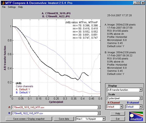
To run MTF Compare (Imatest Master only), press MTF Compare in the upper right of the Imatest Main Window, just below SFR: Current file, which is often grayed out.
CSV input files are selected by pressing the down arrows  on the right of the A and B boxes on the lower left and selecting either Browse... or Recent files, which opens a box containing up to 12 recently used files. The selected files must be CSV output files generated by Imatest SFR.
When both A and B contain valid data, a plot appears, using the saved Display and Scale selections.
Display options
Display controls what is displayed, i.e., the y-axis.
- A/B Transfer function MTF(A)/MTF(B) is displayed a bold solid black line —— up to the lowest frequency where the denominator (MTF(B)) drops below 0.04, and as a thin dashed gray line - - - - at higher frequencies, where noise makes results unreliable. MTF(A) is displayed as a faint brown line ——, and MTF(B) is displayed as a faint blue line ——.
 B/A Transfer function Similar to A/B, except that MTF(B)/MTF(A) is displayed.
 - A strong, B faint MTF(A) is displayed as a strong brown line —— ; MTF(B) is displayed as a faint blue line ——.
- B strong, A faint MTF(B) is displayed as a strong blue line —— ; MTF(A) is displayed as a faint brown line ——.
- Summary and EXIF data displays a summary of the results and EXIF data (available in JPEG files). A portion of this display is shown on the right.
Scale controls the scaling of the display, i.e., the x-axis.
- Cycles/pixel A maximum of 1 is always displayed.
- Line Widths/Picture Height (LW/PH) The maximum value displayed is the lower of the maximum values for A and B. Care must be used in interpreting results because sensors have widely varying heights (measured in number of pixels).
- Cycles/mm Pixel spacing (microns per pixel, pixels per mm, or pixels per inch) must be entered in the SFR input dialog box for both A and B for the cycles per distance scales to be displayed. The maximum value displayed is the lower of the maximum values for A and B. Care must be used in interpreting results because sensors have widely varying pixel spacings and heights.
- Cycles/inch
A and B-channels determine the color channel used for the analysis. The values are not stored between runs: Default is always displayed when MTF Compare starts.
- Default uses the default channel setting that was used and stored in the SFR run. This is typically the Y (Luminance) channel, but it can be any of the others.
- (corr) uses the results for the default channel with Standardized sharpening applied.
- R Red channel.
- G Green channel.
- B Blue channel.
- Y Luminance channel (not yellow). Approximately 0.3*R + 0.59*G + 0.11*B.
Maximum display frequency (located at the bottom of the window between Save data and Exit) is expressed as a fraction of the Nyquist frequency. The default, 2x Nyquist (1 cycle/pixel) shows all frequencies of interest for high performance digital cameras. But Imatest is sometimesused to measure systems that have much broader or rougher transitions, hence poorer high frequency response (for example, scanned printed paper). In such cases, much of the plot would be wasted. Available settings are
- 2x Nyquist (1 cycle/pixel) [the default] shows all frequencies of interest.
- 1x Nyquist (0.50 cycles/pixel)
- 0.5x Nyquist (0.25 cycles/pixel)
- 0.2x Nyquist (0.10 cycles/pixel)
Other controls
Save screen / Display snapshot (shown on the right) saves a snapshot of the screen (the entire MTF Compare GUI window) as a PNG image file. It also allows you to immediately view the snapshot so it can be used a reference for comparing with other results.
File name and Directory at the top of the window set the location of the file to save.
When you check the Open window in an image viewer... box, the current screen will be opened either the system default viewer (if the box under Image viewer is blank) or a viewer/editor of your choice (if the box contains the path name to the viewer/editor). I recommend using Irfanview, which is fast, compact, free, and supports an amazing number of image file formats. Its normal location in English language installations is C:\Program Files\IrfanView\i_view32.exe.
Save data saves MTF Compare calculation results in an Excel-readable CSV file format.
Help opens this web page in a browser window.
Exit closes MTF Compare.
The File dropdown menu has controls that allow you to set the font size (small, normal, or large) and reset the screen size and location to its original values.
The Help dropdown menu has controls that allow you to open this web page in a browser window, register Imatest, and obtain version information.
Another example
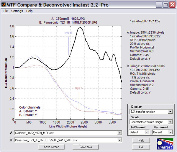
This screen compares two very different cameras— the 8.3 megapixel Canon EOS-20D DSLR (with a high quality 24-70mm lens @ 70mm, f/8, which is about the optimum aperture) and the little 5 megapixel Panasonic Lumix DMC-TZ1 (a tiny camera that sports a 10x Leica zoom lens at f/3.6, which is about optimum for the TZ1's small (1/2.5 inch ≈ 7 mm diagonal) sensor. The test image for the EOS-20D was taken at the Imatest Lab; the image for the TZ1 was downloaded from the Imaging-resource.com website.
Line Widths/Picture Height was chosen for Scale because it best represents total image quality. The picture height (in pixels) is quite similar for the two cameras: 2336 for the EOS-20D; 1920 for the TZ1. MTF Performance of the two cameras is remarkably similar, especially around the 50% level, though the hump in the TZ1's response indicates much stronger sharpening than the EOS-20D (DSLRs tend to use sharpening more conservatively). Indeed, a "halo" is visible near the edge. With additional sharpening the EOS-20D would clearly outperform the TZ1. If Cycles/mm or cycles/inch had been used for Scale, the results would have been harder to interpret because the sensor height is smaller for the TZ1. The pixels are also smaller: 2.2 microns vs. 6.8 microns. (Pixel size does not affect LW/PH mesurements.)
Why, apart from the choice of lenses, bother with the heavy, expensive EOS-20D? Because they differ in a number of other image quality factors beyond simple MTF. The tiny 2.2 micron pixels in the TZ1 have more noise and a smaller dynamic range than the 6.8 micron pixels in the EOS-20D. As important as it is, MTF is not the only game in town.
These tests were repeated in July 2007. The main difference was that we tested a Panasonic DMC-TZ1 in our own lab under similar conditions to the Canon EOS-20D (same target and lighting and same Canon 24-70 mm f/2.8L lens, f/8, 42 mm focal length). The results are remarkably consistent.
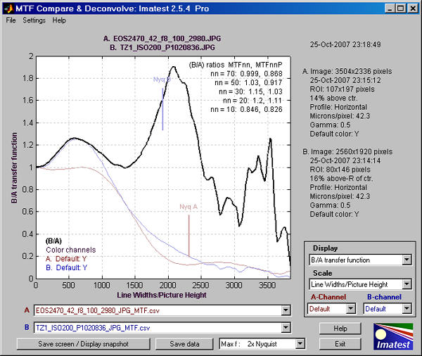
Batchview
Postprocessor for viewing summaries of SFR, SFRplus results
Introduction to Batchview
Batchview is a postprocessor for displaying lens test results generated by SFR and SFRplus batch runs (analyses of groups of test chart images taken at various apertures, focal lengths, etc.). It can store and display up to four sets of results for convenient comparisons in Imatest Master; two in Studio.
Typical use: You've tested a lens at a range of apertures (for example, f/2.8, f/4, f/5.6, f/8, f/11, and f/16) at several focal lengths. To get a good feeling for its performance, you've measured its sharpness (MTF) at the center, corners, and part-way to the corners (ideally, selecting 9 regions). That's a whole lot of data-- 54 MTF curves for each focal length. You want to see a nice, concise summary.
The image below shows MTF50 in Line Widths per Picture Height (LW/PH)— a good measure of total image sharpness)— of four sets of tests (batches of runs).
- (A-C) Two different Canon 17-85mm lenses for a range of apertures at the indicated focal length.
- (D) The Canon 24-70mm f/2.8L.
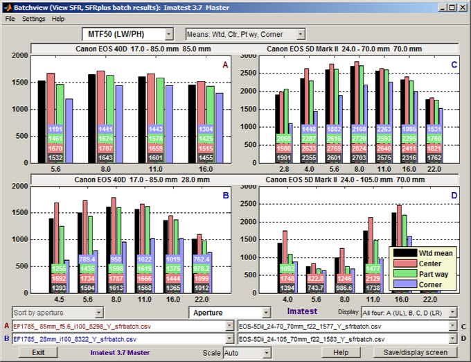
Batchview display from four sets of tests on two lenses:
Canon 17-85mm, 24-70 f/2.8L
Note that the legend (Plot D; lower right) has been moved to uncover the numbers (LW/PH results).
The black, red, green, and blue bars are the weighted mean, the mean of the center region, the mean part-way out, and the mean of the corners, respectively. Numeric values displayed near the base of the bars are optional(they can be turned of in the Settings dropdown menu if desired).
If a single Display is chosen (selected in the Display box on the right, just below the plots), more detail is displayed.
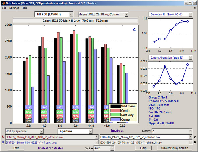
Batchview display from one set of tests:
Canon 17-85mm, 26mm focal length
Two small plots (SMIA TV Distortion and Chromatic aberration area in %) and some EXIF data (metadata) from the first file in the batch are displayed on the right.
Preparing to run Batchview
The first step is to acquire one or more groups of test chart images. By a group we mean a sequence of images in which one parameter is varied (most often aperture, i.e., f-stop, but focal length, ISO speed, etc., could also be varied), usually with other parameters fixed. The chart can be one of the composite charts illustrated in The Imatest Test Lab, but the most convenient and consistent results are obtained with the SFRplus chart, shown below inside the SFRplus setup window in Rescharts, which must be run to save settings prior to doing a batch run for several files in (the automatic, non-interactive version of) SFRplus.
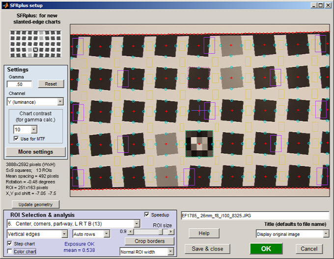
Rescharts SFRplus window showing settings used for the above Batchview run:
9 regions (1 center, 4 part-way, 4 corners)
SFRplus: The following settings are recommended when you run SFRplus in Rescharts. (Full instructions for running Rescharts can be found here).
- Select 9 regions (Center, corners, part-way) for optimum results.
- Chart contrast (typically 10 for SFRplus charts) should be entered. It may be used to calculate the camera gamma used to linearize the image for analysis (the results do not depend strongly on gamma).
- Vertical edges are recommended because they generate better chromatic aberration measurements-- they're close to tangential.
- Open the SFRplus Settings & options window to view settings. Most have no direct effect on Batchview. We recommend checking Close figures after save. The input file to Batchview is always saved for batch runs.
When the settings are correct, click Save settings to save the settings without running SFRplus or click OK to save settings and interactively run the selected file. Then press SFRplus in the Imatest main window and select the batch of files to analyze. A maximum batch size of six is allowed in Imatest Studio.
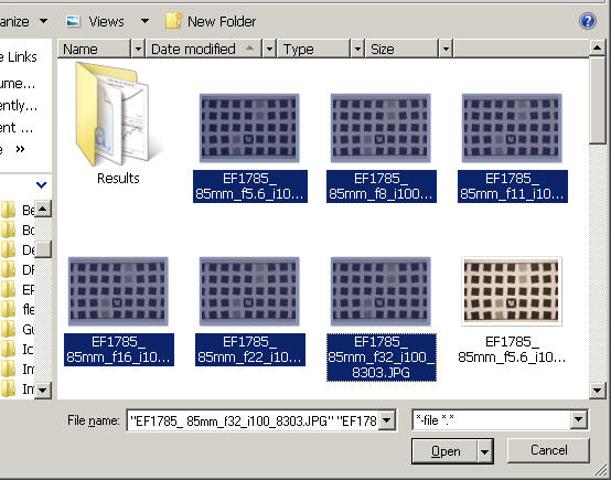
Read images dialog box, showing a batch of 6 files (form f/5.6 to f/32)
Use the View/Rename files module to change the meaningless names generated by the camera to more meaningful names that contain key EXIF data such as the aperture, focal length, etc. The file names in the above illustration were processed through View/Rename files.
SFR can also be used to generate input for Batchview, especially with targets that contain slanted-edges near the center, part-way out, and near the corners. The composite target shown below works quite nicely and also includes the Log F-Contrast and Star charts.
Sharpness target (30x40 inch) for cameras up to about 16 megapixels.
Details in The Imatest Test Lab.
Instructions for running SFR with this chart can be found in Using SFR Part 2. The sections on Repeated runs, Multiple ROI fine adjustment, and Automatic ROI refinement contain some helpful tips.
Running Batchview
To run Batchview, click the Batchview button in the Imatest main window. Initially, a blank screen will appear. In succeeding runs, saved file names will be read in, and a display will appear on the screen.
Empty Batchview opening screen
Enter the batch summary file(s), whose names have the form rootname_chan_sfrbatch.csv, into one of more of the file name windows (A, B, C, or D) at the bottom of the Batchview window. Rootname is typically the root name of the first file in the batch (the file name omitting the extension). Chan is the channel: Y (luminance), R, G, or B.
When files have been entered into the file name window(s) corresponding to the Display menu (lower right), the results will appear. Here is an example showing results for A and B in Imatest Studio.
Batchview results with two displays (Imatest Studio)
A large number of display options are available.
X-axis (independent variable; in the center below the plots)
Sets the independent (X) axis. All except numbers are derived from EXIF data. If EXIF data is not available, the numbers can be added by editing the sfrbatch.csv file in Excel of Open Office.
| Camera |
Camera name |
| Lens |
Lens description |
| ISO Speed |
|
| Focal length |
in mm |
| Shutter speed |
in seconds |
| Aperture |
(same as f-stop) The most commonly used independent variable;
shown in the examples on this page.
|
| Numbers (1,2,3, ...) |
Simple numeric sequence: 1, 2, 3, ... |
Display (lower right)
(both Studio and Master): A, B, A (top), B (bottom). (Master-only): C, D, C (top), D (bottom), All four : A (UL), B, C, D (LR). If a single file is chosen for display, two plots are displayed on the upper right and a summary of EXIF data for the first file is displayed to the right of the image (shown above).
Display variable (dependent variable; left of center above the plots)
This key setting determines what is displayed. The most common choice is MTF50 in Line Widths per Picture Height.
| MTF50 (LW/PH) |
Spatial frequency for where MTF (contrast) is 50%, measured in Line Widths per Picture Height. The best indicator of overall perceptual sharpness of the total image. |
| MTF50 (Cy/Pxl) |
MTF50 measured in Cycles per pixel. Indicates how well pixels are used. |
| MTF20 (LW/PH) |
Spatial frequency for where MTF (contrast) is 20%, measured in LW/PH. Closer to the traditional vanishing resolution (~MTF10) than MTF50. (In digital systems MTF10 is often in the noise or above the Nyquist frequency). |
| MTF20 (cy/Pxl) |
|
| MTF50P (LW/PH) |
Spatial frequency where MTF is 50% of its peak value. The same as MTF50 except for strongly sharpened images, which have a peak in MTF response. Sharpening significantly increases MTF50. MTF50P is somewhat less affected, hence may be a better indicator of the true performance of strongly sharpened imaging systems. |
| MTF50P (Cy/Pxl) |
|
| Peak MTF |
Peak value of MTF. Usually 1, but can be larger for strongly sharpened systems. |
| R1090 (/PH) |
10-90% rise distance of the average edge in units of (10-90%) rises per picture height. Closely tracks MTF50. |
| R1090 (pxl) |
10-90% rise distance in pixels. Approximately inversely proportional to MTF50. |
| LSF PW50 (pxl) |
50% pulse width of the Line Spread Function (derivative of the edge) in pixels. |
| CA (pxl) |
Lateral Chromatic Aberration (LCA) area in pixels. CA area is closely related to its visibility. But area in pixel units is not recommended because it is strongly affected by location. |
| CA (area %) |
LCA area in units of percentage of the distance from the image center to the corner. Somewhat dependent on location, but much less so than when pixels are chosen as the units. May be strongly affected by raw conversion algorithm. |
| CA (crossing %) |
LCA measured by the maximum distance between the transition centers of the three channels in center-to-corner %age. |
| CA (R-G %) |
LCA measured by the distance between the transition centers of the Red-Green channels in center-to-corner %age. |
| CA (B-G %) |
LCA measured by the distance between the transition centers of the Blue-Green channels in center-to-corner %age. |
Display regions
This selects the regions represented by the bars in the plot. The first, which selects a weighted sum (100% center, 75% part-way, 25% corners) and three others is the most common selection, but others may have value.
| Means: Wtd Ctr, Pt wy, Corner |
Display four bars.: The black, red, green, and blue bars are the weighted mean, the mean of the center region, the mean part-way out, and the mean of the corners, respectively. |
| Weighted mean |
One bar displaying the weighted mean. |
| Center mean |
One bar displaying the value in the center. |
| Part way mean, worst |
Two bars displaying the mean and worst-case value, part-way to the corner. (Worst case MTF is the lowest; worst case Chromatic Aberration is the highest). |
| Center mean, worst |
Two bars displaying the mean and worst-case values in the corner region. |
Region locations are shown below.
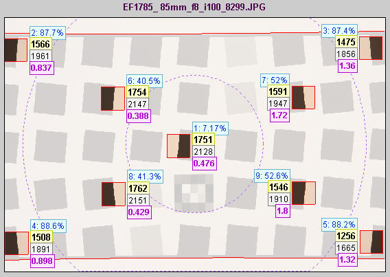
Multi region summary showing center region (inner circle)
and corner region (outside outer circle).
Plots on right (for single batch display)
When a single plot is selected, two small additional plots appear on the right. This enables you to present a rather complete set of results, for example (as shown above), sharpness on the main (large) plot, distortion in the upper-right plot, and chromatic aberration in the middle-right plot. The following parameters are available for the small right plots.
| Distortion % |
SMIA TV distortion in %. Positive is pincushion; negative is barrel. |
| CA (area %) |
LCA area in units of percentage of the distance from the image center to the corner. Somewhat dependent on location, but much less so than when pixels are chosen as the units. May be strongly affected by raw conversion algorithm. |
| CA (crossing %) |
LCA measured by the maximum distance between the transition centers of the three channels in center-to-corner %age. |
| CA (R-G %) |
LCA measured by the distance between the transition centers of the Red-Green channels in center-to-corner %age. |
| CA (B-G %) |
LCA measured by the distance between the transition centers of the Blue-Green channels in center-to-corner %age. |
Using Stepchart
Stepchart analyzes the tonal response,
noise,
and dynamic range of digital cameras and scanners using
Stepchart can also measure veiling glare (lens flare).
New in Imatest 3.1
Highly distorted images can be analyzed if automatic patch location is turned off. Several images can be combined (averaged) to facilitate fixed pattern noise measurement.
New in Imatest 2.7
A new Dynamic Range postprocessor allows dynamic range to be measured from several exposures of a reflective step chart, which can be much more convenient than using a transmission chart. |
The Kodak Q-13 Gray Scale is an 8 inch long
chart
consisting of 20 zones, labeled 0-19, which have optical
densities from 0.05 to 1.95 in steps of 0.1 (reflectances from
0.891
to 0.011). The Kodak Q-14 is identical, except that it's 14 inches long. The chart is printed on a
(semigloss)
surface. The Jessops chart, from the UK, is similar to the Q-13, except that it has only 18 zones.
| This
image of the Q-13 Gray Scale was photographed
slightly out of focus to minimize noise. |
|
The Q-13 has finer steps and a higher maximum density than the
GretagMacbeth
ColorChecker (Dmax = 1.95 vs. 1.5), mostly because of its glossier
surface. It considerably less
expensive. The longer Q-14 is well suited for photographing near ColorCheckers or slanted-edge
SFR
test targets.
Iliah Borg has analyzed the Q-13 Gray Scale. He says, "I'm pretty sure it's screen-printed, most likely with automotive
enamel. The spectral response is flat from 420 to 730nm,
similar to titanium dioxide mixed with carbon in different
proportions to achieve different reflectivities. The layer is
pretty thick, to isolate from the substrate."
Applied Image and ISO targets: Imatest Master
Five monochrome targets, shown below, have been added to Imatest Master with Imatest 1.7. To run them, open the image file, then select the approximate region of interest for the key features in the target, following the instructions in Stepchart with Applied Image/ISO targets. Additional dialog boxes allow you to specify the target type and refine the crop.
|
|
Stepchart also analyzes transmission (i.e., film) charts, which
have higher maximum densities than reflective charts, making them
suitable
for measuring the dynamic range of digital cameras and scanners, as
discussed
below, in the section on Dynamic range.
Photographing
the chart and running Stepchart
- Light. Be sure the light is even and free of glare. As little as
possible
should come from behind the camera— it can cause glare and flatten
image
tones. At least two lamps with an incident angle of about 30° are recommended. A recommended lighting setup is described in The Imatest Test Lab. Be especially careful to avoid glare in the dark zones on the right of the Q-13/Q-14 charts; it can hard to avoid with wide angle lenses. The light should not emphasize the texture of the chart, which would
cause
erroreous noise measurements. If possible, the surroundings of the Step chart should be dark gray or
black to minimize flare light (unless you are measuring flare light).
- Focus. The chart may be photographed slightly
out of focus to minimize noise measurement errors due to texture in the
patches. I emphasize slightly—
the boundaries between the patches must remain distinct.
- Distance. The distance at which the target is photographed is not critical.
The
noise
analysis will be most accurate if the total cropped chart length is at least
1000
pixels (about 50 pixels per zone), about 1/3 the width of the image in
a 6 megapixel digital SLR. Increasing the size improves the accuracy of
the noise measurement up to a point: there is little improvement over 2000 pixels wide. Useful (though less accurate) noise analysis results may be obtained with total cropped length as small as 400 pixels. The tonal response can be measured with very small images, as long as the zones are distinctly visible.
- Photograph the chart.
- Save the image as a RAW file, TIFF, or maximum quality JPEG, then load
it on
your
computer. If you are using a RAW converter, convert to JPEG (maximum
quality),
TIFF (without LZW compression), or PNG. If you
are using film, develop and scan it.
- Run Imatest.
- Click on the Stepchart
button in the Imatest main window.
- Open the input file using the dialog box. Imatest remembers the
directory
name of the last input file opened (for each module, individually).
| Multiple file selection Several files can be selected in Imatest Master using standard Windows techniques (shift-click or control-click). Depending on your response to the multi-image dialog box you can combine (average) several files or run them sequentially (batch mode). |
Combined (averaged) files are useful for measuring fixed-pattern noise (at least 8 identical images captured at low ISO speed are recommended). The combined file can be saved. Its name will be the same as the first selected file with _comb_n appended, where n is the number of files combined. |
Batch mode allows several files to be analyzed in sequence. There are three requirements. The files should (1) be in the same folder, (2) have the same pixel size, and (3) be framed identically. |
The input dialog box for the first run is the same as for standard non-batch runs. Additional runs use the same settings. Since no user input is required they can run extremely fast. |
If the order of the files in a batch runs is different from the selection order, click Settings, Options and Settings... (in the Imatest main window) and change the setting in Batch run order. The sequence may be affected by Windows Explorer settings. |
One caution: Imatest can slow dramatically on most computers when more than about twenty figures are open. For this reason we recommend checking the Close figures after save checkbox, and saving the results. This allows a large number of image files to be run in batch mode without danger of bogging down the computer. |
|
- Crop the image to minimize edge effects. Typical crops (for automatic zone detection) are shown
below, indicated by red rectangles.
Click outside the image for no crop. The orientation does not
need
to be correct; Imatest will rotate the image to the correct orientation. To display the exposure error correctly (for reflective targets only), select the entire chart, including any clipped highlight patches that may be present. If the aspect ratio (length:width) of the crop is less than 4:1, the selection will be rejected (Imatest Studio) or a dialog box for one of the Applied Image/ISO charts will appear (Imatest Master). If you plan to use manual Zone detection (selected in the Stepchart input dialog box, below), the selection can be approximate: a fine selection window will enable you to refine the crop.
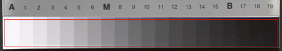
Crop of a Kodak Q-13 chart
.
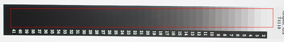
Crop of a Stouffer T4110 chart (better without the tilt).
This is an image processed by Stepchart, after cropping.

- Make any needed changes to the Stepchart input dialog box.
Chart type A
reflective
target with density steps of 0.10 (the Kodak Q-13/Q-14) is selected by
default.
If you are using a transmission target, be sure to choose the correct
target
type. In Imatest Master you can enter a table of densities from an ASCII file (one density per line). Automatic (default) must be unchecked to enable Veiling glare measurements. (See Dynamic range, below.) Click OK to continue.
Stepchart input dialog box
Zone detection You can toggle between Automatic (the default) and Manual Zone detection with the Automatic (default) checkbox. If it is unchecked, a fixed number of patches (6-41) can be selected with the slider for Stepchart analysis, and a fine ROI adjustment box appears after OK is pressed. This option is useful when high noise in dark regions confuses the automatic ROI detection, or when veiling glare is to be calculated. (Zone detection can also be set from Options & Settings in the Imatest main window.)
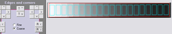
Fine ROI selection (dialog box detail): Details here.
Scaling You can select the minimum value of the x-axis for figures 2 and 3. This setting defaults to Auto. Setting it manually allows several successive runs to be scaled identically, which can clarify comparisons between different cameras.
Results (Fig. 1), Lower plot: Pixel noise Three noise displays are available for the lower-left plot in first figure.
| Noise (%) normalized to image density range = 1.5 |
Values 0-1. Useful because it references the noise to the scene: noise performance is not affected by camera contrast. |
| Noise (%) normalized to 255 pixels |
Values 0-1. Noise will be worse for higher contrast cameras (affected by the gamma encoding) |
| Noise in pixels (maximum of 255) |
Values 0-255. |
Noise Detail (Fig. 2), Middle plot: f-stop noise or SNR Two types of display are available for the middle-left plot of the second figure. The effects of gradual illumination nonuniformities have been removed from the results.
| f-stop noise |
Scene-referenced noise, based on f-stops (factors of 2 in exposure or illumination) |
| SNR (based on f-stops) |
Scene-references Signal-to-Noise Ratio, based on f-stops. Note that there are many ways of defining SNR. Most are image (or pixel)-referenced. Results are different from S/N in the lower plot (which is more standard). |
The scaling (minimum and maximum values) can be set in the dropdown menus to the right of the radio buttons. Most of the time these should be left at Auto. The values are inverted when the display is toggled between F-stop noise and SNR. For example, the minimum value of the x-axis in both Figures 2 and 3 can be set between -4 and -1.5.
Noise Detail (Fig. 2), Lower plot: Pixel noise or SNR Five types of display are available for the lower-left plot of the second figure. The first three are the same as the lower plot of Fig. 1. The effects of gradual illumination nonuniformities have been removed from the noise results. All displays are derived from Noise in pixels (the third selection below). In the notation below Ni is RMS noise and Si is signal (pixel) level for patch i.
| Noise (%) normalized to image density range = 1.5 |
100% * (Noise in pixels) divided by (the difference in pixel levels between light and dark patches that have a density difference of 1.5). This difference is close to the 1.45 White-Black difference in the ColorChecker. Useful because it references the noise to the scene: noise performance is not affected by camera contrast. |
| Noise (%) normalized to 255 pixels (max of 100) |
100% * (Noise in pixels) / 255 = Ni/2.55. Values 0-100. This noise measurement will be worse for higher contrast cameras. (It is affected by the gamma encoding.) |
| Noise in pixels (maximum of 255) |
Noise in pixels ( Ni ). Values 0-255. |
Pixel S/N (Signal in patch/RMS noise) dimensionless
|
Noise in pixels ( Ni ). Values 0-255. |
| Pixel SNR (dB) (20*log10(S/N)) |
20 Log10(signal/noise) for each patch (where signal = pixel level). Units of dB (decibels). Doubling S/N increased dB measurement by 6.02. |
�
For this selection, SNR_BW is also displayed. SNR_BW is an average SNR based on White-Black patches (density difference = 1.5, close to the W-B difference in the ColorChecker).
SNR_BW = 20 log10((SWHITE-SBLACK )/Nmid ), where Nmid is the noise in a middle gray patch (closest to nominal chart density = 0.7). |
Output
The example was photographed with the Canon EOS-10D at ISO 100 and
converted
from RAW format using Capture One with default settings (no curves
applied).
The results include tonal response and noise. Colorcheck
produces a similar result, but with less tonal detail. Three figures are
produced for color images; two for B&W.
First
Figure
The upper plot shows the average density
of the grayscale patches (black curve) and first and second order
density fits (dashed blue and green
curves). The horizontal axis is the distance along the target. A
portion of the patches themselves are shown just above the plot. The
equations
for the density fits are given in the Algorithm section, below. The
second
order fit closely matches the patches. The light cyan spikes are the
differentiated
and smoothed steps used to find the boundaries between zones.
The lower plot shows the RMS noise for
each patch:
R, G, B, and Y (luminance). In this plot it is expressed as the percentage of the pixel level difference corresponding to a target density range of 1.5: the same
as
the white - black patches on the GretagMacbeth ColorChecker. For this camera, the pixel difference is 197.5. For this display, noise measured in pixels can be calculated by multiplying the percentage noise by 197.5.
Noise can also be normalized to 255 pixels or expressed in pixels (maximum of 255). Options are described above.
The high levels of Red and Blue noise in zones 3-6 may be due to
imperfections
in the target which are completely swamped by the noise
at ISO 1600, shown below. Noise is largest in the dark areas because of gamma
encoding: In the conversion from the sensor's linear output to the
color
space (sRGB, here) intended for viewing at gamma = 2.2, the dark areas
are amplified more than the light areas and the noise is boosted as well. |
See Noise in photographic images for a detailed explanation of noise: its appearance and measurement.
Second figure
The second figure (Noise detail) contains some of the
most important results:
- the tonal response curve (displayed on a log
scale, similar to film response curves),
- noise expressed as either a fraction of an f-stop (or EV or zone), or f-stop Signal-to-Noise Ratio (SNR = S/N = 1/f-stop noise),
- noise or SNR (signal-to-noise ratio), based on pixel levels, expressed in one of several ways, and
- dynamic range (for
transmission step charts).
The horizontal
axis for the three plots on the left is Log Exposure, which equals
(minus) the nominal target
density
(0.05 - 1.95 for the Q-13 chart). This axis is reversed from Figure 1.
The upper left plot shows the density (tonal) response (gray squares), as well as the first and second order fits (dashed blue and green lines). It resembles a traditional film density response curve. Dynamic range is grayed out because the reflective Q-13 target has too small a density range to measure a camera's total dynamic range. See Dynamic range, below. This curve is closely related to the Opto-Electronic Conversion Function (OECF), which is a linear curve of exposure vs. pixel level.
|
The upper right box contains dynamic range results: total dynamic range and range for several quality levels, based on luminance (Y) noise. Details below. It is shown in gray when a reflective target is selected. |
Second figure
The x-axis (log exposure) is reversed in direction from Figure 1, which shows the chart zone (from light to dark)

The f-stop Signal-to-Noise Ratio (SNR_f = 1/f-stop noise) can be displayed in the middle-left figure
in place of RMS noise (in f-stops).
|
|
The middle left plot shows noise in f-stops (or EV), i.e., noise scaled to (divided by) the
difference in pixel levels between f-stops, which decreases as
brightness decreases. Noise measured this way is the inverse of the signal-to-noise ratio (N/S), which we will call SNR_f (to distinguish it from other SNR measurements). The darkest levels have the highest noise. This
measurement corresponds to the workings of the eye and has
important consequences for the calculation of practical dynamic range.
The vertical axis is logarithmic to display low noise levels clearly.
Dynamic range information is displayed when the range for a specific
quality level (defined by maximum f-stop noise or minimum S/N) is within the range of the
plot. It is omitted if noise or SNR_f is better than the specified level for all patches: it is not reported for quality levels lower than H in the above plot because the noise level never reaches 0.25 (the M-H level).
The bottom left plot shows pixel noise or SNR scaled in one of several different ways. The above illustration shows pixel noise normalized to the difference in levels between lightest patch and the patch corresponding to a density of 1.5— close to the 1.45 density range as the GretagMacbeth Colorchecker. (The normalization is discussed in Fig. 1, above.)
|
EXIF data is shown in the
middle right region.
The lower right plot shows the noise
spectrum. Digital
camera images with excessive noise reduction will have an unusually
rapid
falloff of the noise spectrum. |
 |
The bottom left plot has several display options, listed above. Pixel SNR (dB) is shown on the left.
SNR (dB) = 20 log10(Si/Ni), where Si is the signal (mean pixel level) of patch i and Ni is the noise (standard deviation of the pixel level, with slow variations removed) of patch i.
SNR_BW is an average SNR based on white-black patches (density difference = 1.5)
SNR_BW = 20 log10((SWHITE-SBLACK )/Nmid ), where Nmid is the noise in a middle level patch (closest to nominal chart density = 0.7). |
 |
Here are the results for ISO 1600. Tonal response is similar to ISO
100,
but the noise is greatly increased— enough to swamp out any
imperfections
in the target. The noise is highly visible. It wouldn't be suitable for
portraits and other high quality work, but it would be acceptable when
a grainy "Tri-X" or "available light" look is desired. Neat
image can do an excellent job of reducing it. The middle-left plot displays
dynamic range for several quality levels, specified by the maximum
noise within the range. The dynamic range for low quality (L; blue) has a maximum noise of 1 f-stop; the dynamic range for high quality (H; yellow) has a maximum noise of 0.1 f-stop. |
Third Figure
The upper plot shows the density response (small circles) of the luminance (Y), red, green, and blue channels, as well as the first and second order fits (dotted and dashed gray lines). It resembles a set of traditional film density response curves. The R, G, and B curves are displayed in Imatest Master only.
For reflection step charts only, the nominal exposure is shown as pink dots (•), and the exposure error in f-stops is displayed. Exposure error is less critical than for ColorCheck, where it strongly affects the a*b* color values: that's why it isn't displayed in the other figures. The equation for nominal exposure is similar to equation that calculates the grayscale pixel levels of the ColorChecker:
pixel level = 255 * (10–density/1.01)(1/2.2)
The lower plot shows the slope of the density curve, which can also be regarded as the local contrast or gamma. This curve is the derivative of the density, d(Density) / d(Log Exposure).
Lens flare (stray light that bounces between lens elements and off the barrel) can be measured by photographing a reflective step chart (a Q-13 or Q-14) against dark and white backgrounds. When flare light is present (white background) it will reduce the slope of the density response in dark regions of the step chart (on the left of the plot). This curve makes it easy to measure the decrease in the slope.
Saving
the results
|
When the Stepchart calculations are complete, the Save Stepchart Results? dialog box appears. It allows you to select figures to save and
choose
where to save them. The default is subdirectory Results
in the data file directory. You can change to another existing
directory,
but new results directories must be created outside of Imatest— using
a utility such as Windows Explorer. (This is a limitation of this
version
of Matlab.) The selections are saved between runs.
You can examine the output figures before you check or uncheck
the boxes.
Figures, CSV, and XML data are saved in files whose names consist of a root file name with a suffix and extension. The root file name defaults to the image file name, but can be changed using the Results root file name box. Be sure to press enter.
Checking Close figures after save is recommended for preventing a buildup of figures (which slows down most systems) in batch runs. After you click on Yes or No,
the Imatest main window reappears. |
 |
Dynamic
range of cameras and scanners
| The Dynamic Range module, introduced in Imatest 2.7, calculates dynamic range from several reflective stepchart images, which are easier to work with than transmission step charts. |
|
Dynamic range (DR) is the range of tones over which a camera responds. It is usually measured in f-stops, or equivalently, zones or EV. (It can also be measured in density units, where one density unit = 3.322 f-stops.) It can be specified in two ways:
- The total range. Stepchart is extremely sensitive at detecting a camera's total dynamic range, even when dark areas are extremely noisy or boundaries between chart zones become indistinct.
- A range of tones over which the RMS noise, measured in f-stops (the inverse of the signal-to-noise ratio, SNR), remains under a specified maximum value. The lower this value (the higher the minimum SNR), the better the image quality but the smaller the dynamic range. Noise tends to be worst in the darkest regions. Imatest calculates the dynamic range for several maximum RMS noise levels, from 0.1 f-stop (high image quality; SNR = 10) to 1 f-stop (low quality; SNR = 1).
The dynamic range corresponding SNR = 1 (1 f-stop of noise) corresponds to the intent of the definition of ISO Dynamic range in section 6.3 of the ISO noise measurement standard: ISO 15739: Photography — Electronic still-picture imaging — Noise measurements. The Imatest measurement differs in several details from ISO 15739; hence the results cannot be expected to be identical. Imatest may well produce more accurate results because it measures DR directly from a transmission chart, rather than extrapolating results for a reflective chart with maximum density = 2.0.
Change in dynamic range definition (Imatest 1.5.5, November 24, 2005)
The definition of total dynamic range now includes indistinct zones (dark zones that the original Stepchart algorithm had difficulty detecting). This may cause some short-term confusion because Figure 2 will change: total DR will sometimes increase. But it better represents true camera performance. |
|
|
A camera's (or scanner's)
dynamic range can be accurately
measured
using a transmission step chart illuinated from behind by a lightbox.
Reflection step charts such as the Kodak Q-13 or Q-14 are inadequate
because
their density range of around 1.9 is
equivalent
to 1.9 * 3.32 = 6.3 f-stops,
well below that of digital cameras.
Transmission step chart
The table below lists several transmission step charts, all of
which
have a density range of at least 3 (10 f-stops). Kodak Photographic
Step
Tablets can be purchased calibrated or uncalibrated. Uncalibrated is
usually
sufficient. The Stouffer charts are attractively priced. |
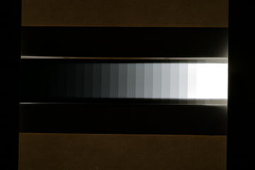 |
The Stouffer T4110 (13.3 f-stops range), Danes-Picta TS28D (13.6 f-stops range), or TE 241 (13.6 f-stops range) are recommended for digital SLRs, which can have dynamic ranges over 10 f-stops. The charts with Dmax = 3.05 = 10 f-stops are probably adequate for compact digital cameras with small pixel sizes (under 3 microns).
Lightbox
You'll need a lightbox that can evenly illuminate the transmission step chart. 8x10 inches is large enough. Avoid thin or "mini" models, which may not have even enough illumination. The Logan Tru-View 810/920 is inexpensive and quite adequate. Light boxes are widely available, though they may be hard to find on dealers' websites. On Adorama, click on Filing/Storage | Mounting & Viewing Equipment | Lightboxes & Loupes. On B&H, click on Projection & Viewing | General Presentation Equipment | Lightboxes, Loupes & Slide Viewers | Lightboxes & Slide Viewers | Lightboxes & Light Tables. T he Kyoritsu calibrated light sources, especially the pattern light boxes, available in the North America from C.R.I.S,, are worth checking out. Image Engineering/E sser Test Charts makes an excellent integrating sphere, ideal for use with the TE 241.
To measure dynamic range,
- Prepare a fixture for mounting the the step chart. It should be
large
enough
to keep stray light out
of
the camera. Stray light can reduce the measured dynamic range; it should be avoided at all costs. I made a fixture out of scrap mat board held together with Scotch
magic tape and Elmer's glue. (That old mainstay, duct tape, wasn't
quite
right for the job.)
- Place the fixture and step chart on top of the lightbox— or any
other
source
of uniform diffuse light.
- Photograph the chart in a darkened room. No stray light should reach the front of the target; it will distort the results. The sourroundings of the chart should be kept as dark as possible to minimize flare light. An example
is
shown
above. The density difference between the darker zones is not very
visible,
but it shows up clearly in the measurements. I used a Kodak step wedge
(density steps of 0.15) that I purchased in 1969!
- Use your camera's histogram to determine the minimum exposure
that
saturates
the lightest region of the chart. Overexposure (or underexposure)
reduces
the number of useful zones. The lightest region should have a relative pixel level of at least 0.98 (pixel level 250 or 255); otherwise the full dynamic range of the camera will not be detected. If the lightest zone is below this level, and a transmission chart is selected, a Dynamic range warning is issued.
- For
flatbed scanners with transparency units (TPUs, i.e., light sources for transparencies), you can simply lay the step chart down on the glass.
Stray light shouldn't be an issue, though there is no harm in keeping
it
to a minimum. 35mm film scanners may be difficult to test since most
can
only scan 36mm segments. (Most transmission targets are longer.) For
scanners
specified as having Dmax greater than 3, the charts of choice are the Stouffer
Transmission Step Wedge T4110 or Danes-Picta TS28D, which are too large to be tested
easily
with 35mm film scanners.
- Follow the remainder of instructions in Photographing
the chart and running Stepchart, above. Be sure to select the
correct chart type from the Stepchart input dialog box (right).
The Imatest algorithm for finding dynamic range is remarkably
accurate.
Imatest detects chart zones using the smallest density step that
results
in uniformly spaced detected zones (see Algorithm).
For smaller steps, noise can be mistaken for zone boundaries. For
larger
steps, fewer zones are detected.
The dynamic range is the difference in
density between the zone where the pixel level is 98% of its maximum value (250 for 24-bit color, where the maximum is 255), estimated by interpolation, and the darkest zone that meets the measurement criterion.
The repeatability of this measurement is better than 1/4 f-stop.
Here is a result for the Canon EOS-10D at ISO 400, converted from
RAW
format with Capture One LE.
|
The
total dynamic range of
the
Canon EOS-10D is 8.6 f-stops. Total dynamic
range
improves slightly for 48-bit TIFF conversion but very little for ISO
100. But the lower noise in 48-bit TIFF conversion and ISO 100 results
in improved dynamic ranges for given quality levels. Cautionary note: This dynamic range is limited by the test chart (an old Kodak Step Tablet with a maximum range of 10 f-stops). A chart like the Stouffer
T4110 might result in a higher number: possibly over 10 f-stops).
The shape of the response curve is a
strong function of the conversion software settings. The plot on the
right
is for Canon Zoom Browser with Contrast set to Low: the transfer curve is very different from
Capture One LE, but the dynamic range is quite close— the result of slightly different noise reduction processing. |
 |
To convert dynamic range from f-stops into decibels (dB), the measurement normally given on sensor data sheets, multiply the dynamic range in f-stops by 6.02 (20 log10(2)). The dynamic range for low quality (f-stop noise = 1; SNR = 1) corresponds most closely to the number on the data sheets. Measured dynamic range is normally somewhat lower than specified dynamic range because of lens flare and other factors.
Summary .CSV and XML files
An optional .CSV (comma-separated variable) output file contains results for Stepchart. Its name is [root name]_summary.csv. An example is Canon_EOS10D_Q13_ISO400_crop_summary.csv.
The format is as follows:
| Module |
SFR, SFR multi-ROI, Colorcheck, or Stepchart. |
| File |
File name (title). |
| Run date |
mm/dd/yyyy hh:mm of run. |
| (blank line) |
| Tables |
Tables are separated by blank lines. |
| The first table contains measured and ideal pixel levels and densities. |
| The second table contains density = -log(exposure) and Y, R, G, and B densities (-log(pixel level/255)), assuming 8 bits/pixel. |
| The third table contains the density differences (slopes) between the Y, R, G, and B patches. |
The fourth table contains two sets of
Y, R, G, and B noise measurements for the the patches in the bottom two rows, described above.
– Noise (%) normalized to image density range = 1.5
– f-stop noise |
| The fifth table contains S/N and SNR (dB) for the Y, R, G, and B channels, described above. |
| (blank line) |
| Additional data |
The first entry is the name of the data; the second (and additional) entries contain the value. Names are generally self-explanatory (similar to the figures). |
| (blank line) |
| EXIF data |
Displayed if available. EXIF data is image file metadata that contains important camera, lens, and exposure settings. By default, Imatest uses a small program, jhead.exe, which works only with JPEG files, to read EXIF data. To read detailed EXIF data from all image file formats, we recommend downloading, installing, and selecting Phil Harvey's ExifTool, as described here. |
This format is similar for all modules. Data is largely self-explanatory. Enhancements to .CSV files will be listed in the Change Log.
The optional XML output file contains results similar to the .CSV file. Its contents are largely self-explanatory. It is stored in [root name].xml. XML output will be used for extensions to Imatest, such as databases, to be written by Imatest and third parties. Contact us if you have questions or suggestions.
| Indistinct zones in the Stouffer T4110 test chart
The Stouffer T4110 test chart is particularly valuable because its maximum density of 4.0 (corresponding to 13 f-stops or a 10,000:1 brightness range) makes it uniquely suitable for measuring the dynamic range of digital SLRs. But the original Stepchart algorithm, which depended on sharp boundaries between zones, sometimes failed to detect zones in the darkest regions. This problem first appeared in dark zones (D > 3.3) of images taken by Max Penson of D-spot (a leading Hebrew language digital photography website) with the Fuji S2 Pro and S3 Pro (which claims an extended dynamic range).
To correct this problem, Stepchart now extrapolates— infers zones in dark areas within the crop, as long as the density in each zone is less than that of the previous zone by at least 0.2 times the average density difference between detected zones. These "indistinct" zones are indicated by light graphics on the left of the plots below. For the Fuji S3 Pro with a "Standard" setting, there are 6 "indistinct" zones, representing 2 additional f-stops, for a total dynamic range of 13 (huge; better than negative film). These numbers are real, and starting with Imatest 1.5.5 (November 2005) they are included in the definition of Total Dynamic Range. The number of indistinct steps (and DR based on distinct steps only) is still displayed, but its significance has been downplayed.
|
| Algorithm |
- (Automatic zone detection only) Locate
the distinct zones in the image. This is done by taking the derivative
of the pixel level averaged vertically, then smoothing it, illustrated
by the light cyan spikes in the upper left plots in the above figures.
A boundary between zones is detected if this function goes above a
threshold.
The threshold is adjusted to the lowest value that gives evenly spaced,
regular intervals. This is an optimum detection
algorithm:
a lower threshold detects false boundaries (i.e., noise), while a
higher
threshold can miss valid zones.
- Find regions
of interest (ROIs) for each zone, which comprises the central 2/3 of
the
zone.
- Calculate
statistics for the ROIs, including the average pixel level and a second-order polynomial fit to the pixel levels inside the ROIs— this fit is
subtracted from the pixel levels for calculating noise. It removes the
effects of nonuniform illumination.
- Calculate
the noise in each ROI. The noise is the standard deviation of the pixel level, after the second-order polynomial has been subtracted. Noise display options are given above. The noise spectrum is calculated for the seventh zone (middle gray) by lining up the pixels (with the second-order polynomial subtracted) into a 1D array and taking the Fourier transform (FFT). The independent axis is displayed in Cycles/pixel, where 0.5 is the Nyquist frequency.
- Using
the average pixel values of the regions whose value is 10% below the
maximum
and above theminum, the average pixel response is fit to a mathematical
function (actually, two functions). This requires some explanation.
- Using
the average pixel values of grayscale zones for densities between
approximately
0.1 and 0.9 (omitting the extremes near white and black), the average
pixel
response is fit to two mathematical functions to find gamma (contrast: first-order equation) and also a second order qeuation.
This
requires some explanation.
A
simplified (first-order) equation for a capture device (camera or scanner) response
is,
normalized
pixel level = (pixel level/255) = k1 exposuregamc
Gamc
is the gamma of the capture device. Monitors also have
gamma
= gamm defined by
monitor
luminance = (pixel level/255)gamm
Both gammas
affect the final image contrast,
System
gamma = gamc * gamm
Gamc is
typically around 0.5 = 1/2 for digital cameras. Gamm is 1.8 for
Macintosh
systems; gamm is 2.2 for Windows systems and several well known color
spaces
(sRGB, Adobe RGB 1998, etc.). Images tend to look best when system
gamma
is somewhat larger than 1.0, though this may not hold for contrasty
scenes.
For more on gamma, see Glossary, Using
Imatest SFR, and Monitor
calibration.
Using
the equation, density = - log10(exposure) + k,
log10(normalized
pixel level) = log10( k1 exposuregamc
) = k2 - gamc * density
This is
a nice first order equation with slope gamc, represented by the blue
dashed curves in the figure. But it's not very accurate. A second order
equation works much better:
log10(normalized
pixel level) = k3 + k4 * density
+ k5 * density2
k3,
k4, and k5 are found using second order
regression
and plotted in the green dashed curves. The second order fit
works
extremely well.
|
|
Stepchart: Applied Image and ISO charts
Applied Image and ISO charts
In addition to linear reflective and transmission step charts, Stepchart (in Imatest Master) can analyze the tonal response and noise of a number of additional charts, all but one of which are available from Applied Image. These charts are described below.
| |
QA-61 |
REFLECTIVE SCANNER TEST CHART (ISO-16067-1) |
| |
Data: |
Size 100mm x 152mm (4in x 6in); Designed to ISO-16067-1 specifications. Includes Landolt Ring, alphanumeric resolution and slant edge charts; grey step patches, horizontal, vertical and slanted ronchi patterns (6 - 40 c/mm) plus the APPLIED T-100 Digital Electronic Pixel target. |
| |
Notes: |
Used for determining reflective light resolution & imaging characteristics of digital scanning systems. For full description, see QA-61 Product specifications. |
| |
|
Part No.
QA-61-ISO-16067-1-P-RP |
Overall Size
102 x 152mm (4 x 6in) |
Material
Reflective Material |
QA-62
|
|
| QA-62 |
SLANT EDGE TARGET Slant Edge Scanner Target with Grayscale SFR & OECF #2 Ideal for evaluation response of digital systems to the slanted sharp edge function and used for MTF analysis. |
| Data: |
Size 75mm x 75mm (3in x 3in); 25mm dark grey square rotated (5 degree) on a light grey background; surrounded by 20 nine-mm square grey scale patches. |
| Notes: |
Ideal for evaluation response of digital systems to the slanted sharp edge function and used for MTF analysis. For full description, see QA-62 Product specifications. |
|
Part No.
QA-62-SFR-P-RP |
Overall Size
95 x 76mm (3.75 x 3in) |
Material
RP - photo paper |
|
ST-51
EIA Grayscale |
|
| ST-51 |
EIA HALFTONE GRAY SCALE |
| Data: |
The EIA grayscale pattern is a standard 2" square projection slide. It contains two parallel gray scales. The upper scale has nine nominally equal transmission steps while the lower contains the same number of nominally equal density steps. The transmission values range from 3% to 60%, corresponding to density values of 1.52 and 0.22 respectively. The slide is chrome on glass and densities are achieved by a fine halftone pattern. Densities can be found here. |
| |
Part No.
ST-51-CG |
Overall Size
50mm x 50mm |
Material
Reflective Material |
|
ST-52
ISO-14524
12-patch
OECF target
(circular)
|
|
| ST-52 |
ISO DIGITAL CAMERA CONTRAST CHART |
| Data: |
This Camera Contrast Chart conforms to International Standard ISO-14524, Photography - Electronic Still Picture Cameras - Methods for Measuring Opto-Electronic Conversion Functions (OECF). |
| Notes: |
Chart features 12 gray levels on a durable material. Densities range from 0.10 to 2.30. |
| |
Part No.
ST-52-RM |
Overall Size
356mm x 200mm |
Material
Reflective Material |
|
ISO-15739
Noise target
|
|
Details on the I3A.org ISO Tools dowload page, particularly the ISO 15739 Noise Test Chart Utility |
20-patch
OECF
targets
(circular)
|
|
Several charts use this 20-patch arrangement.
(upper) Portion of proposed low-contrast ISO 12233 chart
When OECF 20-patch circular is selected in the input dialog box (below), one of the following chart contrasts should be selected in the box just below the OECF 20-patch radio button.
| TE 241 |
Available from Image Engineering/Esser Test Charts. Transmissive chart. 12600:1 contrast ratio. 0 ≤ density ≤ 4.1 |
| Low contrast 20:1 |
From ISO/DIS 14524, Table A3. 0.1 ≤ density ≤ 1.4 |
| Standard reflection 80:1 |
From ISO/DIS 14524, Table A3. 0.1 ≤ density ≤ 2.0 |
| Normal contrast 160:1 |
From ISO/DIS 14524, Table A3. 0.1 ≤ density ≤ 2.3 |
| High contrast 1000:1 |
From ISO/DIS 14524, Table A3. 0.1 ≤ density ≤ 3.1 |
(lower) Esser Test Charts TE241 |
|
| ITE Grayscale |
|
Comes in two versions: Type I: gamma = 0.45 and Type II: gamma = 1.0. Available from DNP (Japan), Zonetech (Korea), and Image Engineering/Esser Test Charts (Germany), where it is designated TE 83 and TE 84.
When ITE Grayscale is selected in the input dialog box (below), either ITE Grayscale I: gamma = 0.45 or ITE Grayscale II: gamma = 1.0 should be selected in the box just above the ITE Grayscale radio button. |
Instructions for Applied Image/ISO charts
Run Stepchart in the usual manner by clicking on Stepchart in the Imatest main window.
Select the approximate crop region, which should include the grayscale patches and no more. Ignore any crop or selection marks. The crop does not have to be accurate; a find adjustment dialog box will appear later. If the crop aspect ratio is less than 3:1, Stepchart recognizes the chart as one of the Applied Image/ISO charts.
Cropping illustration for the five targets
The initial crop should include the grayscale patches and no more. It does not have to be accurate: after the chart type is selected,a fine adjustment dialog box appears.
|
|
The dialog box shown below appears. The cropped input image is shown on the right. Select the appropriate chart type using the radio buttons in the middle. The image on the left illustrates the chart type: the patches should match the input image on the right.
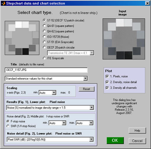
You can change the title if needed. You can select a file for reference density values if you choose not to use the standard values. The file should contain patch densities, one per line. The patch order is given below. The scaling box affects the x-axis and noise plots in Figures 2 and 3. It is identical to the standard Stepchart input dialog box. If you choose OECF 20-patch circular, choose one of the contrast settings listed in the above table.
If you click OK, the fine ROI selection box, shown below appears. You can move the entire ROI using one of the buttons on the top left: ^ , v , < , or > . You can move the top margin with T ^ or T v , the bottom margin with B ^ or B v , etc. Corners can also be adjust individually: useful in the presence of perspective or lens distortion. Author's note: I would have liked to be able to click and drag on lines or corners, but the limitations of the Matlab interface didn't allow this.
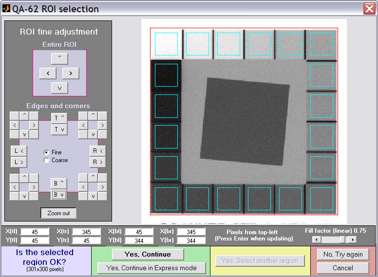
You can enter X and Y values for the corners (tl = top left, etc.): be sure to press Enter for each value if you do. The size of the selection is shown on the lower left. Fill factor (linear) (on the lower right, just above No, Try again ) sets the size of the squares. It defaults to 0.7. It can be increased to obtain more samples for noise analysis, but it may need to be reduced if the image is tilted or distorted. The Distortion slider allows highly distorted (barrel or pincushion) images to be analyzed. Fill factor may have to be reduced in the presence of extreme distortion.
When the squares have been adjusted, click Yes, Continue , No, Try again , or Cancel .
The Output is the same as for standard linear step charts.
Patch order for the five targets
The table below shows the patch order for the targets. Use this order when creating a custom density file.
Orientation and numbering of patches for monochrome targets |
1 2 3 4 5 6
20 7
19 8
18 9
17 10
16 15 14 13 12 11 |
1 2 3 4 5 6
20 7
19 8
18 9
17 10
16 15 14 13 12 11 |
1 2 3 4 5 6 7 8 9
10 11 12 13 14 15 16 17 18 |
1 2
3 4
5 6
7 8
9 10
11 12 |
QA-61 ISO-
16067-1 Scanner |
QA-62 |
ST-51
EIA Grayscale |
ST-52
ISO-14524
OECF target |
3 1 2
5 4
7 6
9 8
11 12 10 |
3 1 2 4
5 6
7 8
9 10
11 12
13 14
15 16
17 19 20 18 |
1 2 3 4 5 6 7 8 9 10 11
12 13 14 15 16 17 18 19 20 21 22 |
|
ISO-15739
Noise target
|
20-patch OECF targets |
ITE Grayscale |
|
Dynamic Range
Calculate Dynamic Range from several Stepchart images
Introduction to Dynamic Range
Thanks for Jonathan Sachs for suggesting this module.
Dynamic Range is a postprocessor for Stepchart that calculates a camera's dynamic range— the range of exposure it can capture at a specified quality level— from up to four exposures of reflective step charts such as the Kodak Q-13 and Q-14. In most instances this approach is more convenient than using a transmission step chart, which requires an even light source and must be photographed in a totally darkened room. As with all Imatest modules, a great many display options are available.
We start by describing the operation of Dynamic Range. Dynamic range is explained in detail below.
Dynamic Range
- reads up to four CSV files created by Stepchart. The files should be the results for four stepchart images taken with the same camera and lens but with exposures separated by 2-4 f-stops.
- aligns the x-axis (log exposure) to represent the relative exposures. The resulting range is far larger than the density range of a single reflective chart— about 6.5 f-stops.
- calculates dynamic range based on f-stop noise used in Stepchart) or pixel noise (calculated in Stepchart but not used for dynamic range).
|
Example of Dynamic range output showing f-stop noise
and corresponding dynamic ranges |
Operation
- Capture several images of a reflective test chart, with each image differing in exposure by 1 or 2 f-stops (EV). The total range from the most to least exposed image should be at least 6 f-stops (7 or 8 doesn't hurt). The least exposed images will appear nearly black, but they should contain some detail. The lightest patch in the most exposed image should be saturated (R, G, and B = 255 in 24-bit color images or 65515 in 48-bit color images. Be sure the light is glare-free. The Imatest Test Lab page has a great many valuable recommendations.
- To determine a camera's ultimate potential, store the image files in RAW format for later conversion. You may also with to capture and store JPEG files for comparison— to see how much dynamic range is lost with in-camera JPEG conversion.
- If RAW images are to be analyzed, convert the to 16-bit TIFF format for best results. You may use any RAW converter. Be sure to record the settings, which affect the tonal response curve. Noise reduction (one of the functions of RAW converters) also has an effect on the measured dynamic range.
- Analyze the images with Stepchart. Be sure to save the CSV output files.
- Open Dynamic Range by clicking on the button on the left of the Imatest main window. The following welcome screen appears. It may contain instructions that are more up-to-date than the image below. Previously-entered CSV files are read and stored.
Dynamic Range opening screen
- Read the CSV results files generated by Stepchart into windows A, B, C, and/or D. (One or two of the windows can be empty. None can be entered if needs be.) The files should be for exposures separated by 2-4 f-stops (EV), with 3 about optimum. The number of detected patches is shown to the right of the window ( N 20 20 17 10 ).
- If results have not already appeared, click on Calculate.
Results
Several displays and display options are available. They are selected in the lower-right region of the Dynamic Range window.
| Display |
| Pixel levels vs. exposure, where exposure = -log10(patch density). |
| Log Pixel levels vs. exposure, where Log denotes log10. |
| Local gamma: d(Log pixel level) / d(Log exposure), i.e., the slope of the Log pixel level plot. Gamma is contrast. |
| f-stop noise: Noise referenced to the image. |
| S/N (1/f-stop noise) |
| SNR (1/f-stop noise) dB = 20 log10(1/f-stop noise). |
| Pixel S/N (Pixel level/noise). Displayed optionally by Stepchart. Referenced to the file. |
| Pixel SNR dB = 20 log10(Pixel level/noise) |
| Exif data |
| Channel |
| (Imatest Master only) Selects color channel: Y (luminance), R, G, or B. |
| X-axis scale |
| f-stops (EV). The most popular units for expressing dyamic range. |
| Density units: Based on a log10 scale. 1 density unit = 3.32 f-stops (EV). |
| X-axis alignment |
| Unshifted |
| Shifted (aligned) Of greatest interest: shows total exposure range |
The image below shows log pixel level vs. (log) exposure (in f-stops). The x-axis has been shifted (aligned). Unaligned log pixel levels are shown as faint lines on the right of the plot. The camera has a strong "shoulder," which reduces the likelihood of highlight burnout.
Log pixel level as a function of (log) exposure. Canon EOS-20D, ISO 100, Standard picture mode.
Dynamic range results are shown on the upper right. Dynamic range numbers based on f-stop noise are shown boldface. These are identical to the numbers in the Stepchart analysis. An alternative dynamic range measurement based on pixel SNR is shown in normal (not bold) typeface. Two additional plots are shown below. The number of detected patches for each file is shown to the right of the file name ( N 20 20 17 10 ).
f-stop noise, showing dynamic ranges
Pixel SNR in dB (20 log10(Pixel level/noise)), showing dynamic ranges
Dynamic range — background
Dynamic range (DR) is the range of tones over which a camera responds. It is usually measured in f-stops, or equivalently, zones or EV, all of which represent factors of two in exposure. (It can also be measured in density units, where one density unit = 3.322 f-stops.)
DR is typically specified as the range of tones over which the RMS noise, measured in f-stops (the inverse of the signal-to-noise ratio, SNR), remains under a specified maximum value. The lower the maximum noise (the higher the minimum SNR), the better the image quality, but the smaller the corresponding dynamic range. SNR tends to be worst in the darkest regions. Imatest calculates the dynamic range for several maximum RMS noise levels, from 0.1 f-stop (high image quality; SNR = 10) to 1 f-stop (low quality; SNR = 1).
The dynamic range corresponding SNR = 1 (1 f-stop of noise) corresponds to the intent of the definition of ISO Dynamic range in section 6.3 of the ISO noise measurement standard: ISO 15739: Photography — Electronic still-picture imaging — Noise measurements. The Imatest measurement differs in several details from ISO 15739; hence the results cannot be expected to be identical. Imatest produces more accurate results because it measures DR directly from a sequence of chart images, rather than extrapolating results from a single reflective chart image.
F-stop noise
The human eye responds to relative luminance differences. That's why we think of exposure in terms of zones, f-stops, or EV (exposure value),
where a change of one unit corresponds to halving or doubling
the exposure.
The eye's relative sensitivity is expressed by the Weber-Fechner
law,
ΔL ≈ 0.01 L –or– ΔL/L ≈ 0.01
where ΔL is the smallest luminance difference the eye can distinguish. (This equation is approximate; effective ΔL tends to be larger in dark areas of scenes and prints due to visual interference from bright areas.)
|
|
Expressing noise in relative luminance units, such as f-stops, corresponds more closely to the eye's response than standard pixel or voltage units. Noise in f-stops is obtained by dividing the noise in pixels
by the number of pixels per
f-stop. (I use "f-stop" rather than "zone" or "EV" out of habit; any of them are OK.)
noise in f-stops (EV) = noise in pixels / (d(pixel)/d(f-stop)) = 1/SNR
where d(pixel)/d(f-stop) is the derivative of the pixel level with respect to luminance measured in f-stops (log2(luminance) ). SNR is the Signal-to-Noise Ratio. |
The above-right image illustrates how the pixel spacing between f-stops (and hence d(pixel)/d(f-stop)) decreases with decreasing brightness. This causes f-stop noise to increase with decreasing brightness, visible in the figures above.
Since
luminance noise (measured in f-stops) is referenced to relative scene luminance,
independently of electronic processing or pixel levels, it is a universal measurement
that can be used to compare digital sensor quality when sensor RAW data is unavailable. |
Using Colorcheck
New in Imatest 3.1
Highly distorted images can be analyzed if automatic patch location is turned off. Several images can be combined (averaged) to facilitate fixed pattern noise measurement.
New in Imatest 3.0
Options and Settings I in the Imatest main window allows you to select between traditional ROI selection, which automatically locates patches, and a Multicharts-like method, with adjustable patch locations that are visible during fine adjustment. This can be helpful with distorted images.
New in Imatest 2.6.8
CIEDE2000 color differences (ΔC 2000 and ΔC 2000 have been added.
New in Imatest 2.3.17
Several new options for displaying noise and SNR (Signal-to-Noise Ratio) are described here. |
What Colorcheck does
Colorcheck analyzes images of the widely-available
X-RiteTM (formerly GretagMacbethTM
) ColorChecker®
(available from Adorama and other sources) for color accuracy, tonal response (using the six grayscale patches), and noise or SNR (Signal-to-Noise ratio). Results for tonal
response
are similar to Stepchart. It is particularly useful for measuring the effectiveness of White Balance algorithms and settings under a variety of lighting conditions. The ColorChecker can be photographed in isolation or as part of a scene. Algorithms and equations can be found in the Colorcheck Appendix. The X-Rite ColorChecker is an 8x11" inch chart consisting of 24 patches with 18 familiar colors and six grayscale levels with optical densities from 0.05 to 1.50; a range of 4.8 f-stops. The colors are not highly saturated. The quality of the chart is very high— each patch is printed separately using carefully controlled pigments. Patches have a smooth matte surface. It is available from ColorHQ, Adorama and many other dealers. A 2.25"x3.25" mini ColorChecker is also available. It is useful for including in scenes for evaluating white balance.
| Version comparison |
| Studio: |
Tonal response and noise analyses for B&W patches; La*b* color error and Color analysis |
| Master: |
User-supplied reference files; noise analysis for R, G, B, C, M, and Y patches; noise spectrum |
A simulated ColorChecker is shown below for sRGB color space (the Windows/Internet standard). The optical densities (–log10(reflectivity)) of the grayscale patches on the bottom row are shown in parentheses. One color, patch 18. Cyan, is out of the sRGB gamut; hence it can't be reproduced perfectly on most monitors.
Simulated GertagMacbeth™ ColorChecker Color Rendition chart

1.
dark
skin
|
2.
light
skin
|
3.
blue
sky
|
4.
foliage
|
5.
blue
flower
|
6.
bluish
green
|
7.
orange
|
8.
purplish
blue
|
9.
moderate
red
|
10.
purple
|
11.
yellow
green
|
12.
orange
yellow
|
13.
blue
|
14.
green
|
15.
red
|
16.
yellow
|
17.
magenta
|
18.
cyan
|
19.
white
(.05)
|
20.
neutral
8 (.23)
|
21.
neutral
6.5 (.44)
|
22.
neutral
5 (.70)
|
23.
neutral
3.5 (1.05)
|
24.
black
(1.50)
|
| What colors are the ColorChecker? |
|
Before 2005 the ColorChecker came with insufficient information. Grayscale densities (for the bottom row)
were
printed on the back of the chart. CIE xyY values (from the familiar 1931 xy chromaticity chart) were included, but these were for CIE illuminant C, whose 6774K color temperature is slightly different from standard 6550K color spaces. A set of RGB values with no specified color space were also included. They should not be used. A ColorChecker purchased in October 2005 had better information: sRGB values and CIE L*a*b* D50 (5000K) values. L*a*b* and RGB values for known color spaces are used in the Imatest analysis. (sRGB is the RGB standard color space for website display.) xy chromaticity values (from the 1931 chart) are far from
perceptually
uniform, i.e., distances between points on the xy-plane are not
proportional
to perceptible differences between colors. (Green is greatly
exaggerated.)
Color differences are better represented in the CIELAB color
space,
where L* is luminance, a* is color on a green-red scale, and b* color on a blue-yellow scale. A distance of 1 between L*a*b* values represents the minimum
perceptible
difference (just-noticeable difference, JND) between colors (for relatively unsaturated colors). For
colors
on the a*b* plane (neglecting L*), this distance is expressed by the equation,
ΔC* = ( (a2*-a1*)2+ (b2*-b1*)2 )1/2 ; where (...)1/2 denotes square root.
More generally,
ΔE*ab = ( (L2*-L1*)2+ (a2*-a1*)2+ (b2*-b1*)2 )1/2 (includes L* differences)
Although ΔC and ΔE*ab (which are both Euclidian distances) are widely used to quantify
color differences, they are not as accurate as the CIE 1994 and CMC equations, which are discussed in detail in the Colorcheck Appendix.
Danny Pascale/Babelcolor's page on the Colorchecker contains everything you want to know about the chart. A great resource! |
| Colorchecker reference values |
|
There are several
sources, each slightly different. The values used by Imatest are shown below.
- The
GretagMacbeth website (now X-Rite) no longer has downloads available. The very best source is Danny
Pascale/BabelColor's RGB
coordinates of the Macbeth ColorChecker is an outstanding resource that contains X-Rite's and Pascale's most recent Colorchecker values (2005). They are very close, with mean ΔE =2. Pascale presents ColorChecker values in xyY, L*a*b*, and a variety of color spaces,
based on numerous measurements. He also presents
procedures
and equations for data conversion. The L*a*b* values are for D50
illumination.
- BruceLindbloom.com contains equations and tables for converting between various RGB color
spaces as well as XYZ, xyY, and CIELAB. Click on Math.
His ColorChecker
values are based on accurate spectrophotometer measurements of a
single
sample. He has a useful ColorChecker
calculator.
- Bruce
Fraser, Creativepro.com. Calibrating
Camera Raw in Photoshop CS contains Bruce's ColorChecker L*a*b* values
from his book, Real
World Color Management. I not sure what
reference
color temperature he uses. Allen
Pacheco has published a similar calibration technique.
The ColorChecker reference can be selected in Colorcheck. At present you may choose between references 1 (X-Rite) and 3 (Pascale), or you can read L*a*b* or xyY files. The default is the
X-Rite L*a*b* values. The grayscale values are derived from the definition of ISO speed for digital sensors, as described in the Colorcheck Appendix. |
|
Photographing the target and running Colorcheck
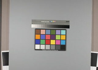 Photograph the ColorChecker. The distance is not critical. There is no need to fill the frame with the ColorChecker image; it is often useful to include other charts or scene elements that can affect white balance.
A ColorChecker image width of 500 to 1500
pixels is sufficient for the Colorcheck noise analysis.
That's about half of the horizontal field of a 6 megapixel SLR. More pixels just slow the calculations. As few as 100 pixels is adequate for color and white balance (but not noise) analysis.
Photograph the ColorChecker. The distance is not critical. There is no need to fill the frame with the ColorChecker image; it is often useful to include other charts or scene elements that can affect white balance.
A ColorChecker image width of 500 to 1500
pixels is sufficient for the Colorcheck noise analysis.
That's about half of the horizontal field of a 6 megapixel SLR. More pixels just slow the calculations. As few as 100 pixels is adequate for color and white balance (but not noise) analysis.
The image on the right shows an image of the ColorChecker and a Q-14 stepchart with a neutral gray surround (similar to the classic 18% gray card), which should help ensure a normal (auto) exposure. Charts tend to be overexposed when the background is black and underexposed when it is white. Still life scenes can be used as backgrounds for testing a camera's automatic white balance (AWB) algorithm.
Lighting should be as even as possible; as
little as possible should come from behind the camera— it can cause
glare.
An angle of incidence of about 30-45 degrees is ideal. For the noise analysis, the
light
should not emphasize the texture of the chart surface, which could affect noise measurements made in
grayscale
patches in the bottom row. More that one light source
is recommended. If possible, the surroundings of the ColorChecker should
be black or gray to minimize flare light. Middle gray (18-22% reflectance) is best for getting the correct exposure with auto-exposure cameras. Uneven lighting tilts
the
tops of the gray scale pixel plot (the upper left plot in the first
figure, below). Lighting uniformity can be measured with an illuminance (Lux) meter. A detailed description of the recommended lighting setup can be found in The Imatest Test Lab. If the objective of running ColorCheck is to analyze a camera's white balance and color accuracy (and no noise analysis is required), the ColorChecker does not need to be photographed under ideal conditions. It can be part of a scene that challenges the camera's white balance algorithm. - If possible, the exposure should be within 1/4 f-stop of the correct value. L*a*b* color values are only accurate if exposure is correct. The exposure error is displayed in several Colorcheck figures. An explanation of exposure and grayscale levels can be found in the Colorcheck Appendix.
- Colorcheck measures the effectiveness of white balance algorithms; results are sensitive to the type of lighting. Outdoor, flash, incandescent, and fluorescent lighting may produce different results. Lighting and Color by John Beale illustrates some of the differences.
- The ColorChecker may be photographed slightly out of focus to minimize errors in noise measurement due to texture in
the patch surfaces. I emphasize slightly—
the dark bands between the patches should remain distinct. The texture
is quite low. If the lighting is reasonably diffuse (not a point
source),
noise from the surface texture should be minimal.
- WARNING The ColorChecker image should not be too large!
Images over 3000 pixels wide (6 megapixels total) can slow calculations because Imatest uses double precision math, which consumes 24
bytes per 3-color pixel. For example, an image from a 6 megapixel camera requires 144 megabytes (6x3x8
MB) in Matlab: enough to bog down computers with limited memory (256 MB or
less). Be especially careful not to fill the frame with 8+ MB digital cameras.Save the image as a RAW file or maximum quality JPEG, then load
it on
your
computer. If you are using a RAW converter, convert to JPEG (maximum
quality),
TIFF (without LZW compression, which is not supported), or PNG.
If
you are using film, develop and scan it.Open Imatest. Click on the Colorcheck
button in the Imatest main window. Open the input file using the dialog box. Imatest remembers the
folder
name of the last input file opened.
| Multiple file selection Several files can be selected in Imatest Master using standard Windows techniques (shift-click or control-click). Depending on your response to the multi-image dialog box you can combine (average) several files or run them sequentially (batch mode). |
Combined (averaged) files are useful for measuring fixed-pattern noise (at least 8 identical images captured at low ISO speed are recommended). The combined file can be saved. Its name will be the same as the first selected file with _comb_n appended, where n is the number of files combined. |
Batch mode allows several files to be analyzed in sequence. There are three requirements. The files should (1) be in the same folder, (2) have the same pixel size, and (3) be framed identically. |
The input dialog box for the first run is the same as for standard non-batch runs. Additional runs use the same settings. Since no user input is required they can run extremely fast. |
If the order of the files in a batch runs is different from the selection order, click Settings, Options and Settings... (in the Imatest main window) and change the setting in Batch run order. The sequence may be affected by Windows Explorer settings. |
One caution: Imatest can slow dramatically on most computers when more than about twenty figures are open. For this reason we recommend checking the Close figures after save checkbox, and saving the results. This allows a large number of image files to be run in batch mode without danger of bogging down the computer. |
|
- Crop the image. The method depends on settings that can be accessed by clicking Options and Settings I in the Imatest main window.
For Automatic patch detection: Original method, crop by dragging the cursor so a small amount of the dark boundaries
at the
edges of the Colorchecker image are visible. There is
no harm if the boundaries are cut off as long as most of the patch area
remains; precise cropping is not critical. Click outside the
image
for no crop. Correct orientation isn't required; Imatest will
rotate the image (in multiples of 90 degrees) to the correct
orientation. This method works well for well-behaved images with little perspective or lens distortion.
The image shown above is representative of a good crop of a well-behaved image.
For Display patch squares in fine adjustment (similar to Multicharts), the initial crop is similar to the original method: drag the cursor so a small amount of the dark boundaries are visible. You'll be able to to refine the boundaries in the fine adjustment window, which is described in detail in Multicharts. For highly distorted images like the one shown below, you'll need to adjust the distortion slider and reduce the fill factor below the default value of 0.7. Since this image has geometrical distortion as well as strong barrel distortion, the corner positions had to be adjusted with care.
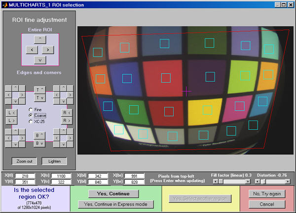
Fine adjustment of a highly distorted image. Corners, Fill factor,
and Distortion were carefully adjusted (they interact somewhat).
- The Imatest Colorcheck dialog box appears if Express mode has not been selected. It allows you change Title, Colorchecker reference, Color space, Noise display, Color error display, and several other parameters from their default values. It also contains news about the latest updates.
Title: defaults to the file name. You can leave or modify it. Figure selection is in the Plot box on the right.
Colorchecker reference selects the ideal ColorChecker L*a*b* and RGB values. You can choose between any of several standard values (based on measurements) or you can enter your own measured values from CSV files. The Old / New radio buttons affect the X-Rite and Babelcolor reference values (described below). Old selects the original reference values, used prior to the release of Imatest 1.6.17 in July 2006. New (recommended) uses more accurate recent measurements. For most color patches, the difference between the old and new values is small.
Standard values:
- X-Rite (default): L*a*b* values provided by X-Rite/GretagMacbeth. Old: Values (formerly on their website) measured with Illuminant C (6774K). New: Values supplied courtesy of X-Rite in 2006 (measured in 2005). Either D50 (5000K) or D65 (6500K) values are used, depending on the white point of the selected color space (below). This is the default.Babelcolor: Values measured by Danny Pascale of Babelcolor. If New is selected, Pascale's D50 values are transformed to D65 using the Bradford transformation for color spaces with a D65 white point. Another excellent choice, close to the X-Rite values. These values, as well as the old and new X-Rite values, are described in Danny Pascale's RGB coordinates of the MacBeth ColorChecker, which is strongly recommended for all Colorcheck users.
- Danes-Picta BST4D: A knockoff of the Colorchecker (same geometry with somewhat different colors) from Danes-Picta in the Czech Republic (on their Digital Imaging page).
Enter your own values: These can be (a) measured on your own instruments or (b) values you have determined to be "pleasing" that you wish to use as design targets. (Remember, accurate color is not necessarily pictorially pleasing. Designers of consumer cameras often aim for "pleasing" colors, which typically involves increasing saturation in foliage, skies, and skin.)
- LAB data file: Read a file containing L*a*b* data. This is the best approach if you have spectrophotometer measurements for your individual chart. A dialog box appears for entering the filename. The file must consist of 24 lines with L*, a*, b* values on each line separated by spaces, commas (,), or semicolons (;). Example (first 3 lines of 24):
38.08, 12.09, 14.39
66.38, 13.22, 17.14
51.06, 0.38, -22.06
(The commas are optional if spaces are present & vice-versa.) If you have an Excel .CSV file with extra rows or columns, you can easily edit it Excel by selecting the key region (3 columns, 24 rows), copying it to a new file, and saving it in .CSV format. L*a*b* data is preferred to xyY data below because it is independent of white point color temperature, hence less error-prone.
- xyY 5000K data file: Read a file containing xyY data with a white point of 5000K (D50). Procedure and format is the same is the LAB data file, above. xyY 6500K data file: Read a file containing xyY data with a white point of 6500K (D65). Procedure and format is the same is the LAB data file, above.
- Last (selected) file: Always appears when the previous selection was an LAB or xyY data file, above.
The Colorchecker reference is displayed at the bottom of the L*a*b* color error figure. |
Noise display: Pixel noise or SNR selects the noise display for the lower-left plot of the first figure (noise/SNR for grayscale row 4) and the upper-right plot of the second figure. (noise/SNR for BGRYMC row 3). The effects of gradual illumination nonuniformities have been removed from the results. All displays are derived from Noise in pixels (the third selection below). The five display types are identical to the types in the lower noise detail plot in Stepchart. In the notation below Ni is RMS noise and Si is signal (pixel) level for patch i.
Noise (%) normalized to White - Black (Zone 19 - 24)
|
100% * (Noise in pixels) divided by (White patch (19) pixel level − Black patch (24) pixel level) =
100% N/(SWHITE−SBLACK ). Useful because it references the noise to the scene: noise performance is not affected by camera contrast. |
| Noise (%) normalized to 255 pixels (max of 100) |
100% * (Noise in pixels) / 255 = Ni/2.55. Values 0-100. This noise measurement will be worse for higher contrast cameras. (It is affected by the gamma encoding.) |
| Noise in pixels (maximum of 255) |
Noise in pixels ( Ni ). Values 0-255. |
Pixel S/N (Signal in patch/RMS noise) dimensionless
|
(Signal (pixel level)) / Noise = Si/Ni for each patch. Dimensionless. |
| Pixel SNR (dB) (20*log10(S/N)) |
20 Log10(Signal/Noise) for each patch = 20 log10( Si/Ni ). Units of dB (decibels). Doubling S/N increased dB measurement by 6.02. |
For this selection, SNR_BW is also displayed. SNR_BW is an average SNR based on White-Black patches (Zone 19 - Zone 24; density difference = 1.45).
SNR_BW = 20 log10((SWHITE-SBLACK )/Nmid ), where Nmid is the noise in patch 22 (the 4th patch in row 4; middle gray; nominal density = 0.7). |
Color space: You can select among the following. Danny Pascale's A Review of RGB Color Spaces is recommended for readers interested in an in-depth explanation of color spaces.
| sRGB |
The default space of Windows and the Internet. Limited color gamut based on typical CRT phosphors. Gamma = 2.2 (approximately), White point = 6500K (D65). |
| Adobe RGB (1998) |
Medium gamut, with stronger greens than sRGB. Often recommended for high quality printed output. Gamma = 2.2, White point = 6500K (D65). |
| Wide Gamut RGB |
Extremely wide gamut with primaries on the spectral locus at 450, 525, and 700 microns. One of the color spaces supported by the Canon DPP RAW converter. 48-bit color files are recommended with wide gamut spaces: banding can be a problem with 24-bit color. Gamma = 2.2, White point = 5000K (D50). |
| ProPhoto RGB |
Extremely wide gamut. Gamma = 1.8, White point = 5000K (D50). Described in RIMM/ROMM RGB
Color Encodings by
Spaulding, Woolfe and Giorgianni. |
| Apple RGB |
Small gamut. Used by Apple. Gamma = 1.8, White point = 6500K (D65). |
| ColorMatch RGB |
Small gamut. Used by Apple. Gamma = 1.8, White point = 5000K (D50). |
Color error display: You can select between
- Standard ΔC and ΔE*ab (CIE 1976) measurements, CIE 1994 measurements (somewhat more accurate), and CMC mesurements (widely used in the textile industry) color difference formulas.
- CIEDE2000 measurements ( ΔC00 and ΔE00 ). The emerging standard. See Gaurav Sharma's CIEDE2000 Color-Difference Formula page.
The CIE-94, CMC, and CIEDE2000 mreasurments reflect the eye's reduced sensitivity to hue and saturation changes for highly saturated colors. Mean CIE-94 numbers are typically around half of the standard measurements; CMC measurements are between the two. CIEDE2000 measurements will be become more familiar as time passes. Patch for noise spectrum (Imatest Master only): You can select any of the patches in the bottom two rows for calculating the noise spectrum. (Row 3 contains B, G, R, Y, M, and C primaries; row 4 contains grayscale values.) The spectra for the Y (luminance), R, G, and B channels is displayed. The third patch in row 4 (middle gray; density = 0.44) is the default. a*b* color error: The upper-right of the a*b* color error plot displays mean color errors (ΔC... and ΔE...) and either the standard deviation of the color error (σ) or the maximum color error (max), selected in this box.
Output
The example was photographed with the Canon EOS-10D at ISO 400, and RAW
converted with Canon FVU using automatic color balance.
The
first figure: Gray scale tonal response and noise
shows graphic results derived
from
the grayscale patches in the bottom row, including tonal
response
and noise. Selected EXIF data is displayed, if available.
The upper left plot is the density
response
of the
colorchecker (gray squares). It includes the first and second order
fits
(dashed blue and green lines). The horizontal axis is Log Exposure (minus the target
density), printed on
the
back of the ColorChecker. Stepchart provides a more detailed
density response curve. The exposure error is shown in pale red if it is less than 0.25 (the maximum recommended error) and bold red otherwise. |
The upper right plot shows the noise in the
third colorchecker row, which contains the most strongly colored
patches: Blue, Green, Red, Yellow, Magenta, and Cyan. In certain
cameras noise may vary with the color. Problems may be apparent that
aren't visible in the gray patches. Note that the x-axis scale (log exposure) is reversed from the plots on the left. |
The lower left plot shows the RMS noise or SNR (signal-to-noise ratio) for
each patch:
R, G, B, and Y (luminance). Several display options are described above. The selected display in the above figure is Noise (%) normalized to White - Black (Zone 19 - 24), i.e., RMS noise is expressed in percentage of
the
difference
between the white and black patches.The average R, G, B, and Y noise for the
gray
zones (2-5) is also reported. |
The lower right region displays EXIF data, if
available. |
 |
The bottom left plot has several display options, listed above. Pixel SNR (dB) is shown on the left.
SNR (dB) = 20 log10(Si/Ni), where Si is the signal (mean pixel level) of patch i and Ni is the noise (standard deviation of the pixel level, with slow variations removed) of patch i.
SNR_BW is an average SNR based on White - Black patches (patch 19 - patch 24; density difference = 1.45)
SNR_BW = 20 log10((SWHITE-SBLACK )/Nmid ), where Nmid is the noise in patch 22 (the 4th patch in row 4; middle gray; closest to nominal chart density = 0.7). |
Two precautions when working with figures
Too many open Figures
Figures can proliferate if you do a number of runs, especially SFR runs with multiple regions, and system performance suffers if too many Figures are open. You will need to manage them. Figures can be closed individually by clicking X on the upper right of the Figure or by any of the usual Windows techniques. You can close them all by clicking Close figures in the Imatest main window. Checking Close figures after save is recommended for batch runs to prevent buildup of open figures. |
Clicking on Figures during calculations
can confuse Matlab. Plots can appear on the wrong figure (usually distorted) or disappear altogether. Wait until all calculations are complete— until the Save or Imatest main window appears— before clicking on any Figures. |
The
second figure: Noise detail (Imatest Master only)
shows the density response, noise in f-stops (a relative measurement
that corresponds to the workings of the eye), noise for the third
Colorchecker row, which contains primary colors, and the noise spectrum of the selected patch.
The upper left plot is the density
response
of the
colorchecker (gray squares). It includes the first and second order
fits
(dashed blue and green lines). The horizontal axis is Log Exposure (minus the target
density), printed on
the
back of the ColorChecker. Stepchart provides a more detailed
density response curve. The exposure error is shown in pale red if it is less than 0.25 (the maximum recommended error) and bold red otherwise. |
The upper right plot shows noise or SNR in the
third Colorchecker row, which contains the most strongly colored
patches: Blue, Green, Red, Yellow, Magenta, and Cyan. Several display options are described above. In certain
cameras noise may vary with the color. Problems may be apparent that
aren't visible in the gray patches. |
The lower left plot shows the R, G, B, and Y
(luminance) RMS noise for as a function of Log Exposure
each patch. RMS noise is expressed in f-stops, a relative measure that
corresponds closely to the workings of the human eye. This measurement
is described in detail in the Stepchart tour. It is largest in the dark areas because the pixel
spacing between f-stops is smallest. |
The lower right plot shows the R, G, B, and Y noise spectrum
of the selected patch. The 3rd patch in the bottom row (a middle gray) has beem selected. The spectrum conveys clues about
signal processing, for example, an unusually rapid rolloff
may indicate excessive noise reduction. The high levels or red and blue noise at low spatial frequencies is typical of Bayer sensors. The ISO speed and Exposure time
from the EXIF data are displayed, if available. |
The
third figure: a*b* Color error
illustrates the color error in
the
device-independent CIELAB color space, where a* is the horizontal axis
and b* is the vertical axis. The squares are the ideal (a*, b*)
ColorChecker
values, set by the ColorChecker reference setting, above. The
circles are the (a*, b*) values of the actual measured
ColorChecker.
The numbers near the squares or circles correspond to the numbers of
the
ColorChecker patches: 1-6 are in the top row, 7-12 are in the second
row,
and 13-18 are in the third row. The numbers for patches 19-24 (the
bottom
row) are omitted because their (a*, b*) values cluster around (0, 0).
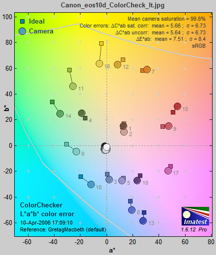
The background of the chart shows expected colors (in monitor sRGB
color
space) for L* around 0.9. It presents a reasonable picture of the
hues associated with a* and b* (though they shift somewhat with L*). The light gray curve is the boundary of the color space (sRGB). There is significant scatter in the
results
because the luminance (L*) of the color patches (not displayed) varies
considerably. This 2-Dimensional figure cannot display L*; a limitation is overcome in Multicharts, which has a rotatable 3D L*a*b* display. CIELAB (often shortened to LAB) was designed to be perceptually
uniform,
meaning that the perceived difference between colors is approximately proportional to
the Euclidian distance between them, ΔE*ab (which includes luminance L*) or ΔC* (color only; omitting L*).
ΔE*ab = ( (L2*-L1*)2+ (a2*-a1*)2+ (b2*-b1*)2 )1/2; ΔC* = ( (a2*-a1*)2+ (b2*-b1*)2 )1/2
The smallest
perceptible
difference corresponds roughly to ΔE*ab = ΔC = 1. (Gaurav Sharma uses 2.3 in the Digital Color Imaging Handbook, p. 31.) CIELAB is far from perfect in
this regard. ΔE*ab for the minimum perceptible color difference
increases
with chroma (i.e., distance from the origin, (a*i2 + b*i2 )1/2. More accurate color difference difference formulas, ΔE*94, ΔE*CMC, and ΔE00, can be selected for display and are included in the CSV and XML output files. If you report any of the more accurate formulas, remember that they are less familiar than plain old ΔE*ab, so to avoid misunderstanding, be sure to clearly indicate which formula you are using. Mean values of ΔE*94 are about half of ΔE*ab . Mean values of ΔE*CMC are between the two. The CIEDE2000 color difference formula, ΔE00, is the emerging standard. It's the most accurate, but it's very complex and still relatively unfamiliar. It's the best choice in the long run. ΔE*94, ΔE*CMC, and ΔE00 are discussed in the Colorcheck Appendix.Several values are reported on the upper right of the figure.
- Mean camera chroma (%) is the average
chroma of camera colors divided by the average chroma of the ideal
Colorchecker colors, expressed as a percentage. The chroma of an individual color is its
distance
from the origin, C = (ai*2+bi*2)1/2. Chroma is often referred to as saturation because more chromatic colors appear to be more saturated. The mean chroma is,
Chroma = 100% mean((a*i_meas2 + b*i_meas2)1/2 ) / mean((ai_ideal*2 + bi_ideal*2)1/2 ) ;
i_meas denotes measured values of patch i; i_ideal denotes ideal ColorChecker values ;
i ≤ 1 ≤ 18 (the first three rows of the Colorchecker) ; mean(x) = Σxi / n for n = 18 values of x.
Chroma is boosted when Chroma > 100%. Chroma
is affected by lens quality (flare light in poor lenses decreases
it)
and signal processing. Many
cameras and most RAW converters have adjustments for
chroma (usually labelled Saturation).
Chroma is not a strong
indicator
of image quality because it is often altered during RAW conversion and can be easily adjusted in image editors.
Images
out of cameras often have boosted saturation to make them more vivid (120% is not
uncommon in compact digital cameras), but boosted saturation can cause a loss of detail in highly saturated objects. Saturation over 120% should be regarded as excessive.
ΔC is color error with luminance difference omitted, i.e., color only. ΔE includes luminance difference. Imatest displays two values of ΔC: with and without correction for the saturation boost (or cut) in the camera, discussed below. You may select between three models of ΔC and ΔE for the display (all are included in the CSV/XML output files).
- Standard ΔC and ΔE*ab measurements, CIE 1994 measurements (somewhat more accurate), and CMC mesurements (widely used in the textile industry) color difference formulas
- CIEDE2000 measurements ( ΔC00 and ΔE00 ). The emerging standard. See Gaurav Sharma's CIEDE2000 Color-Difference Formula page.
ΔC or ΔE of around 1 (2.3 according to Sharma) correspond roughly to a just noticeable difference (JND) between colors. The three color difference models are described in the Colorcheck Appendix. The CIE 1994 and CMC formulas are more accurate than the standard ΔE formula; the CIEDE2000 formulas are the most accurate.
- Color error ΔC is calculated with and without chroma (saturation) correction. Saturation correction involves normalizing the measured colors so their average saturation is the same as the ideal average saturation. This is done by multiplying a*, b*, and C* by 100/Sat. The corrected values, denoted by i_corr, are substituted for the measured values in the ΔC calculation.
a*i_corr = 100 a*i_meas / Sat ; b*i_corr = 100 b*i_meas / Sat
Ci_corr =(a*i_corr2 + b*i_corr2 )1/2
ΔCi_corr = |Ci_corr - Ci_ideal | = ( (a*i_corr - a*i_ideal )2 + (b*i_corr - b*i_ideal )2 )1/2 (Standard (CIE 1976) formula)
This normalization removes the effects of saturation boost, resulting in a lower mean color error, mean(ΔCi_corr ). It is applied because saturation can be easily adjusted by turning a (digital) knob in an image editor. The remaining error, mean(ΔCi_corr ), is a useful indicator of color quality because it cannot be easily removed and it is not a function of mean saturation. It is displayed in
two ways on Figure 3:
- The mean and root mean square (RMS) or maximum color errors are displayed.
mean(x) = Σxi / n for n values of x.
RMS(x) = σ(x) = ( Σxi2 / n )1/2 for n values of x.
x is ΔCi and ΔCi_corr for Colorchecker patches 1-18 (the top three rows).
mean color error (uncorrected) = mean( ΔCi )
mean color error (corrected) = mean( ΔCi_corr )
The root mean square (RMS) error, denoted by sigma (σ), gives greater weight to
large errors; it may therefore be a better overall indicator of color
accuracy. You can select between σ and maximum in the input dialog box.
- Summary: Figure 3 displays the mean and RMS values of the color errors, using either standard (CIE 1976), CIE 1994, or CMC color difference formulas. (The latter two are somewhat more accurate.) CIE 1994 and CMCreflect the eye's reduced sensitivity to hue and especially saturation changes for highly saturated colors. Hence they are generally lower. The results are summarized below.
| ΔC, ΔE display |
One of these four columns is selected. |
The mean and RMS values of all three rows are displayed. |
| ΔC*ab sat. corr. |
ΔC*94 sat. corr. |
ΔC*CMC sat. corr. |
ΔCoo sat. corr. |
Color difference, omitting luminance, corrected for average saturation. |
| ΔC*abuncorr. |
ΔC*94 uncorr. |
ΔC*CMC uncorr. |
ΔCoo uncorr. |
Color difference, omitting luminance; no saturation correction. |
| ΔE*ab |
ΔE*94 |
ΔE*CMC |
ΔEoo |
Color difference, including luminance; no saturation correction. |
It's difficult to assess these numbers until a large database
of test results is available. For now I would characterize the values of ΔC*ab(corr) mean = 5.66
and σ = 6.73 for the EOS-10D (above) as very good to excellent.
| When you interpret the results, keep the following in mind.
Camera manufacturers don't necessarily aim for accurate color reproduction, which can appear flat and dull. They recognize that there is a difference between accurate and pleasing color: most people prefer deep blue skies, saturated green foliage, and warm, slightly saturated skin tones. Ever mindful of the bottom line, they aim to please. Hence they often boost saturation, especially in blues, greens, and skin tones. |
See the Links, below, for details on CIELAB color
space.
The fourth figure: Color analysis
is an image of the ColorChecker
that
allows you to compare the actual and ideal values. It also displays
White
Balance error using the bottom row (the grayscale patches).
The outer portion (1) of each patch contains the ColorChecker image as photographed, The inner portion contains the ideal ColorChecker values corrected for exposure (2) and uncorrected (3).
- The outer region, is
the
patch as photographed. This corresponds to the circles in the L*a*b*
color
error plot, above.
- The square in the
center,
is the ideal value of the patch, corrected
for the luminance of the photographed chart. The
correction
is derived from the second order fit to the gray areas, described
above.
The average luminance of zones 1 and 2 should be close— zone 2 may be
darker
in some patches and lighter in others. Zones 2 and 3 correspond to the
small
squares in the L*a*b* color error plot, above. The exposure error is shown on the same line as the date and color space. Best results are obtained if it is less than 0.25 f-stops.
- The small rectangle
to
the right of the central square, is the ideal value of the patch, with no luminance correction. The luminance of zone 2 will be consistently
lighter
or darker than zone 3 for all patches, depending on the exposure.
|
 |
In the above example, the ColorChecker image
1
is slightly underexposed; it is darker than the ideal uncorrected color
3.
It is also darker than the corrected ideal color 2.
This is a characteristic of this camera: it tends to darken oranges and
lighten blues and cyans. This can be seen in the above right
ColorChecker
image, which is slightly overexposed. This image of the orange-yellow
patch
(row 2, column 6) has about the same luminance as the uncorrected ideal
color 3, but is darker than the corrected ideal color. The uncorrected
ideal value 3 in the two orange-yellow images above (the example on the left and the
full chart on the right) are the same, but appear to be quite different
because of the interaction of colors in the eye— an effect that should
be familiar to artists and photographers.
This image provides a clear visual indication of color accuracy. The L*a*b* color error plot provides a quantitative indication.
The bottom of the third figure illustrates the White
Balance error, which is quantified in three ways. (1)
Saturation
S in the
HSV
color model (burgundy). S can take
on values between 0 for a perfect neutral gray and 1 for a totally
saturated
color. (2) Correlated color temperature error in Degrees Kelvin (blue),
calculated
from Color
Science: Concepts and Methods, Quantitative Data and Formulae,
by Günther Wyszecki and W. S. Stiles, pp. 2224-228. (2)
Color
temperature in Mireds (micro-reciprocal degrees) (blue),
where Mireds = 106/(Degrees Kelvin) is a more perceptually
uniform
measure.
White Balance error tends to be most visible in the gray patches
(2-5
in the bottom row). It is barely visible for S < 0.02. It is quite
serious
for S > 0.10, particularly for the lighter gray patches.
 |
The image at the bottom shows the bottom row (the
grayscale patches)
with exaggerated white
balance
error, calculated by boosting saturation S using the curve on the left,
keeping H and V constant. Low values of saturation are boosted by a
factor
of 4; the boost decreases as saturation increases. This image shows the
White Balance error much more clearly than the unexaggerated chart.
Keep it in mind that this image is worse than reality;
small
White Balance errors may not be obvious in actual photographs,
especially
in the vicinity of strongly saturated colors. |
Saving the
results
|
When the Colorcheck calculations are complete, the Save Colorcheck results? dialog box appears. It allows you to choose
which results to save and where to save them. The default is
subdirectory Results
in the data file directory. You can change to another existing
directory,
but new results directories must be created outside of Imatest— using
a utility such as Windows Explorer. (This is a limitation of this
version
of Matlab.) The selections are saved between runs.
You can examine the output figures before you check or uncheck
the boxes.
After you click on Yes
or No,
the Imatest main window reappears. Figures, CSV, and XML data are saved in files whose names consist of a root file name with a suffix and extension. The root file name defaults to the image file name, but can be changed using the Results root file name box. Be sure to press enter. The .CSV summary file contains Excel .CSV output for the tone
level,
noise, and color calculations. It also contains some additional data,
including
EXIF data for JPEG files. The XML output file contains similar results.
Checking Close figures after save is recommended for batch runs to prevent buildup of open figures. |
 |
Summary .CSV and XML files
An optional .CSV (comma-separated variable) output file contains results for Colorcheck. Its name is [root name]_summary.csv. An example is Canon_EOS10d_ColorCheck_lt_small_summary.csv.
The format is as follows:
| Module |
SFR, SFR multi-ROI, Colorcheck, or Stepchart. |
| File |
File name (title). |
| Run date |
mm/dd/yyyy hh:mm of run. |
| (blank line) |
| Tables |
Tables are separated by blank lines. |
| The first table contains ideal and measured pixel levels and densities. Zone is the chart patch (19-24 for grays). Gray is 1-6, corresponding to patches 19-24. Pixel is the measured pixel level (maximum = 255). Pixel/255 is the normalized measured pixel level. Px/255 ideal is the ideal normalized pixel level. Log(exp) is (-)patch density. Log(px/255) is the log exposure. WB Err Deg and WB Err Mired are white balance errors in degrees and mireds (micro reciprocal degrees), respectively. |
| The second table contains noise measurements for the R, G, B, and Y channels for the the patches in the bottom two rows. Noise is measured in both % of the maximum density patch (19) of the Colorchecker (density = 1.5) and f-stops. |
| The third table contains S/N and SNR (dB) measurements, described above. |
| The fourth table contains ideal and measured RGB and La*b* values for the 24 patches. |
| The fifth table contains several color error measurements (differences with the ideal Colorchecker values) for the 24 patches: ΔC (color difference, neglecting luminance L), ΔE (total difference, including L) using measured (camera) values with and without saturation correction. Details in the Colorcheck Appendix. |
| (blank line) |
| Additional data |
The first entry is the name of the data; the second (and additional) entries contain the value. Names are generally self-explanatory (similar to the figures). |
| (blank line) |
| EXIF data |
Displayed if available. EXIF data is image file metadata that contains important camera, lens, and exposure settings. By default, Imatest uses a small program, jhead.exe, which works only with JPEG files, to read EXIF data. To read detailed EXIF data from all image file formats, we recommend downloading, installing, and selecting Phil Harvey's ExifTool, as described here. |
This format is similar for all modules. Data is largely self-explanatory. Enhancements to .CSV files will be listed in the Change Log.The optional XML output file contains results similar to the .CSV file. Its contents are largely self-explanatory. It is stored in [root name].xml. XML output will be used for extensions to Imatest, such as databases, to be written by Imatest and third parties. Contact us if you have questions or suggestions.
Links
RGB
coordinates of the Macbeth ColorChecker by Danny Pascale, BabelColor, 2003 (PDF). Excellent survey of color spaces and techniques
for
calculating the RGB values of the ColorChecker. And don't forget his other Colorchecker pageBruce
Lindbloom Outstanding site with equations for converting
between color spaces and models. Slightly different L*a*b* values from
Pascale.Earl
F. Glynn (EFG) has an excellent description of the ColorChecker.
His Computer Lab and
Reference
Library are a goldmine of information about color, image
processing,
and related topics.
Lighting and Color by John Beale illustrates how different light sources affect Colorcheck results.Munsell Color Science Laboratory (at RIT) has an interesting page of color standards data available for download, including the spectral reflectivities of the Colorchecker measured by Noboru Ohta. CIE Fundamentals for Color Measurements by Yoshi Ohno, Optical Technology Division, NIST. An excellent review of CIE colorimetry from an IS&T technical conference. Describes the CIE 1931 (x, y) and 1976 (u’v’) diagrams. Digital Color Imaging by Gaurav Sharma A comprehensive 1997 review paper that was updated and turned into the first chapter of the Digital Color Imaging Handbook.
Color management equipment/supplies
ColorHQ.com | ColorManaged.com
GretagMacbethTM and ColorChecker® are tradmarks of X-Rite, Incorporated, which is not affiliated with Imatest. ColorChecker L*a*b* values are supplied courtesy of X-Rite.
Colorcheck Appendix
Algorithms and reference formulas
This page contains algorithms and reference formulas for Colorcheck. It's all in green text because it's all math.
Color difference (error) formulas
The notation in this section is adapted from the Digital Color Imaging Handbook, edited by Gaurav Sharma, published by the CRC Press, referred to below as DCIH. The DCIH online Errata was consulted.
In measuring color error, keep it in mind that accurate color is not necessarily the same as pleasing color. Many manufacturers deliberately alter colors to make them more pleasing, most often by increasing saturation. In calculating color error, you may choose not to use the exact formulas for ColorChecker L*a*b* values; you may want to substitute your own enhanced values. Imatest Master allows you to enter values from a file written in CSV format.
Absolute differences (including luminance)
CIE 1976
The L*a*b* color space was designed to be relatively perceptually uniform. That means that perceptible color difference is approximately equal to the Euclidean distance between L*a*b* values. For colors {L1*, a1*, b1*} and {L2*, a2*, b2*}, where ΔL* = L2* - L1*, Δa* = a2* - a1*, and Δb* = b2* - b1*,
ΔE*ab = ( ( ΔL*)2 + (Δa*)2 + (Δb*)2 )1/2 (DCIH (1.42, 5.35); (...)1/2 denotes square root of (...) ).
Although ΔE*ab is relatively simple to calculate and understand, it's not very accurate expecially for strongly saturated colors. L*a*b* is not as perceptually uniform as its designers intended. For example, for saturated colors, which have large chroma values (C* = ( a*2 + b*2 )1/2 ), the eye is less sensitive to changes in chroma than to corresponding changes for Hue (ΔH* = ( (ΔE*ab)2 - (ΔL*)2 - (ΔC*)2 )1/2 ) or Luminance (ΔL*). To address this issue, several additional color difference formulas have been established. In these formulas, just-noticeable differences (JNDs) are represented by ellipsoids rather than circles.
CIE 1994
The CIE-94 color difference formula, ΔE*94, provides a better measure of perceived color difference.
ΔE*94 = ( (ΔL*)2 + (ΔC*/SC )2 + (ΔH*/SH )2 )1/2 (DCIH (5.37); omitting constants set to 1 ), where
SC = 1 + 0.045 C* ; SH = 1 + 0.015 C* (DCIH (1.53, 1.54) )
[ C* = ( ( a1*2 + b1*2 )1/2 ( a2*2 + b2*2 )1/2 )1/2 (the geometrical mean chroma) gives symmetrical results for colors 1 and 2. However, when one of the colors (denoted by subscript s) is the standard, the chroma of the standard, Cs* = ( as*2 + bs*2 )1/2, is preferred for calculating SC and SH. The asymmetrical equation is used by Bruce Lindbloom.]
ΔH* = ( (ΔE*ab)2 - (ΔL*)2 - (ΔC*)2 )1/2 (hue difference ; DCIH (5.36) )
ΔC* = ( a1*2 + b1*2 )1/2 – ( a2*2 + b2*2 )1/2 (chroma difference)
An early meeting of the
CMC Standards Committee
CMC
The CMC color difference formula is widely used by the textile industry to match bolts of cloth. Although it's less familiar to photographers than the CIE 1976 geometric distance ΔE*ab , it's probably the best of the measurement metrics. It is slightly asymmetrical: subscript s denotes the standard (reference) measurement. CMC is the Color Measurement Committee of the Society of Dyers and Colourists (UK). |
 |
ΔE*CMC(l,c) = ( (ΔL*/lSL)2 + (ΔC*/cSC )2 + (ΔH*/SH )2 )1/2 (DCIH (5.37) ), where
(That's the lowercase letter l in (l,c) and the denominator of (ΔL*/lSL)2.) ΔE*CMC(1,1) (l = c = 1) is used for graphic arts perceptibility mesurements. l = 2 is used in the textile industry for acceptibility of fabric matching. For now Imatest displays ΔE*CMC(1,1).
SL = 0.040975 Ls* / (1+0.01765 Ls*) ; Ls* ≥ 16 (DCIH (1.48) )
= 0.511 ; Ls* < 16
SC = 0.0638 Cs* / (1+0.0131 ) + 0.638 ; SH = SC (TCMC FCMC + 1 - FCMC ) (DCIH (1.49, 1.50) )
FCMC = ( ( Cs*)4 / ( ( Cs*)4 + 1900 ) )1/2 (DCIH (1.51);
TCMC = 0.56 + | 0.2 cos(hs* + 168°) | 164° ≤ hs* ≤ 345° (DCIH (1.52) )
= 0.36 + | 0.4 cos(hs* + 35 °) | otherwise
ΔH* and ΔC* have the same formulas as CIE-94.
CIEDE2000
The CIEDE2000 formulas (ΔEoo and ΔCoo ) are the upcoming standard, and may be regarded as more accurate than the previous formulas. We omit the equations here because they are described very well on Gaurav Sharma's CIEDE2000 Color-Difference Formula web page. Default values of 1 are used for parameters kL, kC, and kH.
At the time of this writing (February 2008) the CIE 1976 color difference metrics (ΔE*ab...) are still the most familiar. CIE 1994 is more accurate and robust, and retains a relatively simple equation. ΔE*CMC is more complex but widely used in the textile industry. The complexity of the CIEDE2000 equations (DCIH, section 1.7.4, pp. 34-40) has slowed their widespread adoption, but they are on their way to becomming the accepted standard. For the long run, CIEDE2000 color difference metrics are the best choice.
Color differences that omit luminance difference
Since Colorcheck measures captured images, exposure errors will strongly affect color differences ΔE*ab, ΔE*94, and ΔE*94. Since it is useful to look at color errors independently of exposure error, we define color differences that omit ΔL*.
ΔC*ab = ((Δa*)2 + (Δb*)2 )1/2
ΔC*94 = ( (ΔC*/SC )2 + (ΔH*/SH )2 )1/2
ΔC*CMC = ((ΔC*/SC )2 + (ΔH*/SH )2 )1/2
ΔC00 omits the ( ΔL'/kLSL )2 term from the ΔE00 (square root) equation (see Sharma).
These formulas don't entirely remove the effects of exposure error since L* is affected by exposure, but they reduce it to a manageable level.
| Notation changes (made for consistency with textbooks such as DCIH) |
ΔC*ab = ((Δa*)2 + (Δb*)2 )1/2, formerly called ΔE(a*b*), is the color difference (only), with L* omitted.
ΔE*ab = ( ( ΔL*)2 + (Δa*)2 + (Δb*)2 )1/2, formerly called ΔE(L*a*b*), is the total difference, including L*.
This notation is somewhat confusing because ΔE*ab includes L* (as well as a and b) in its formula. |
Color differences corrected for chroma (saturation) boost/cut
Many digital cameras deliberately boost chroma, i.e., saturation, to enhance image appearance in digital cameras. This boost increases color error in the ΔE and ΔC formulas, above.
The mean chroma percentage is
Chrp = 100% * (measured mean( (ai*2+bi*2)1/2 ) ) / (Colorchecker mean( (ai*2+bi*2)1/2 ) )
= 100% * mean (Cmeasured) / mean (Cideal) ; Ci = (ai*2+bi*2 )1/2
i ≤ 1 ≤ 18 (the first three rows of the Colorchecker)
Chroma, which is closely related to the perception of saturation, is boosted when Chrp > 100. Chroma boost increases color error measurements ΔE*ab, ΔC*ab, ΔE*94, and ΔC*94. Since it is easy to remove chroma boost in image editors (with saturation settings), it is useful to measure the color error after the mean chroma has been corrected (normalized) to 100%. To do so, normalized ai_corr and bi_corr are substituted for measured (camera) values ai and bi in the above equations.
ai_corr = 100 ai / Chrp ; bi_corr = 100 bi / Chrp
The reference values for the ColorChecker are unchanged. Color differences corrected for chroma are denoted ΔC*ab(corr), ΔC*94(corr), and ΔC*CMC(corr).
Mean and RMS values
Colorcheck Figure 3 reports the mean and RMS values of ΔC*ab corrected (for saturation) and uncorrected, where
mean(x) = Σxi / n for n values of x.
RMS(x) = σ(x) = (Σxi2 / n )1/2 for n values of x.
The RMS value is of interest because it gives more weight to the larger errors.
Algorithm
- Locate the regions of interest (ROIs) for the 24 ColorChecker zones.
- Calculate statistics for the six grayscale patches in the bottom row, including the average pixel levels and a second order polynomial fit to the pixel levels in the ROIs— this fit is subtracted from the pixel levels for calculating noise. It removes the effects of nonuniform illumination. Calculate the noise for each patch.
- Using the average pixel values of grayscale zones 2-5 in the bottom (omitting the extremes: white and black), the average pixel response is fit to a mathematical function (actually, two functions). This requires some explanation.
A simplified equation for a capture device (camera or scanner) response is,
normalized pixel level = (pixel level/255) = k1 exposuregamc
Gamc is the gamma of the capture device. Monitors also have gamma = gamm defined by
monitor luminance = (pixel level/255)gamm
Both gammas affect the final image contrast,
System gamma = gamc * gamm
Gamc is typically around 0.5 = 1/2 for digital cameras. Gamm is 1.8 for Macintosh systems; gamm is 2.2 for Windows systems and several well known color spaces (sRGB, Adobe RGB 1998, etc.). Images tend to look best when system gamma is somewhat larger than 1.0, though this doesn't always hold— certainly not for contrasty scenes. For more on gamma, see Glossary, Using Imatest SFR, and Monitor calibration.
Using the equation, density = - log10(exposure) + k,
log10(normalized pixel level) = log10( k1 exposuregamc ) = k2 - gamc * density
This is a nice first order equation with slope gamc, represented by the blue dashed curves in the figure. But it's not very accurate. A second order equation works much better:
log10(normalized pixel level) = k3 + k4 * density + k5 * density2
k3, k4, and k5 are found using second order regression and plotted in the green dashed curves. The second order fit works extremely well.
- Saturation S in HSV color representation is defined as S(HSV) = (max(R,G,B)-min(R,G,B))/max(R,G,B). S correlates more closely with perceptual White Balance error in HSV representation than it does in HSL.
The the equation for saturation boost in the lower image of the third figure is S' = (1-e-4S )/(1-e-4), where e = 2.71828...
Grayscale levels and exposure error
The Colorchecker grayscale patch densities (in the bottom row) are specified as 0.05, 0.23, 0.44, 0.70, 1.05, and 1.50. Using the equation, pixel level = 255 * (10–density/1.06)(1/2.2) (see ISO speed, below), the ideal pixel levels would be 236, 195, 157, 119, 83, and 52, about 3% lower than the values measured by Bruce Lindbloom (242, 201, 161, 122, 83, and 49 for the Green channel) and provided with a Colorchecker purchased in October 2005 (243, 200, 160, 122, 85, 52). On the average, these measured values fit the equation,
pixel level = 255 * (10–density/1.01)(1/2.2)
Exposure error is measured by comparing the measured levels of patches 2-5 in the bottom row (20-23 in the chart as a whole) with the selected reference levels. Patches 1 and 6 (19, 24) are omitted because they frequently clip. Since pixel level is proportional to exposuregamma, and hence log10(exposure) is proportional to log10(pixel level) / gamma (where gamma is measured from patches 2-5), the log exposure error for an individual patch is
Δ(log exposure) = (log10(measured pixel level) - log10(reference level)) / gamma
Using the mean value of Δ(log exposure) for patches 2-5 and the equation, f-stops = 3.32 * log exposure,
Exposure error in f-stops = 3 32 * (mean(log10(measured pixel level) - log10(reference level))) / gamma
ISO speed
ISO speed is defined in Kodak Image Sensors - ISO Measurement (App note MTD/PS-0234), which is extracted from ISO standard 12232:1998. (Only 73 CHF— about $60 US— for 131 kB; such a deal!)
There are two basic types of ISO measurement: saturation-based (also called "base") and noise-based. The saturation-based ISO, which corresponds to the lowest camera ISO setting, is
ISO = (15.4 * f#2) / (L * t) [Exposed so an 18% gray card has a level 18/106 of full scale. See below.]
where f# is the effective f-number of the camera lens, L is the luminance in cd/m2 of an 18% reflector (the familiar 18% gray card), and t is the exposure time in seconds. A camera's effective ISO setting may be increased by increasing the electronic gain.
You can use this equation to find the approximate luminance of an object, L = (15.4 * f#2) / (ISO * t), where f# and t are read from an 18% gray card. For a typical white surface (90% reflectance), L = (3.08 * f#2) / (ISO * t).
Digital image sensors are linear devices: their output voltage (and the pixel level in a RAW image file) is proportional to the light energy reaching the pixel up to the point where it abruptly saturates. Now here's the heart of the matter.
When an exposure is made according to the above setting, an 18% gray card has a voltage or pixel level 18/106 of full scale. In an 8-bit color space encoded for display at gamma = 2.2 (sRGB, Adobe RGB, WGRGB, etc.), the corresponding pixel level is 114 (from the formula, pixel level = 255*(18/106)(1/2.2) ). Of course this is an ideal value; pixel levels in real cameras may vary, especially when a tonal response "S" curve is applied.
Any portion of the image with luminance equivalent to more than 106% reflectiance (5.9x brighter than the gray card) will be saturated-- pure white; burnt out; gonzo. Since a white card is about 90% reflectance (density = 0.05), that doesn't leave much margin. The Kodak document says, "Very demanding applications might need more headroom for highlights, and so might use a higher number when calculating base ISO." That's why exposure compensation-- equivalent to increased ISO speed-- is often required to avoid burnt out highlights for "very demanding applications" like ordinary sunlit outdoor scenes.
Using Multicharts
Interactive analysis of several test charts
Introduction
|
|
|
|
|
|
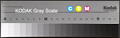
Q-13 |
|
|
Imatest™ Multicharts analyzes images of several test charts for color accuracy and tonal response using a highly interactive user interface. It can be used to measure white balance and color response for a wide range of lighting conditions and scenes. It can also display the tonal response of monochrome charts (or monochrome portions of color charts). A color correction matrix can be calculated (Imatest Master only).
Several of the supported test charts are shown on the left. The 140-patch ColorChecker SG, ChromaDuMonde, linear grayscale stepcharts, and several additional Special Charts are supported by Imatest Master only. |
Getting started
Photograph or scan the chart, taking care to avoid glare, which can be problematic in charts with semigloss (SG) and glossy surfaces such as the IT8.7 and ColorChecker SG. Glare can be especially difficult to control with wide angle lenses. A recommended lighting setup is described here. For testing white balance, you can photograph the chart in a scene under a variety of lighting conditions. The mini ColorChecker is especially suitable for this purpose. Rectangular charts may be rotated by multiples of ±90° if they are geometrically symmetrical (these include the two ColorCheckers, the CMP DT003, QPCard 01, and the Kodak Q-13/Q-14, but not the IT8.7 (where top and bottom are different).
To start Multicharts, run Imatest, then click the Multicharts button. The Multicharts window will appear with brief instructions, which may be more up-to-date than the ones shown below.
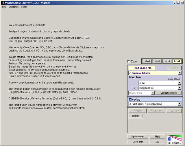
| Select a chart to analyze by clicking on one of the entries in the popup menu below Chart type or by clicking on Read image file if the correct Chart type is displayed. The Read image file button and popup menu (shown on the right) are highlighted (yellow background) when Multicharts starts. Multicharts supports the following charts: |
 |
| The standard 24-patch X-Rite ColorChecker®. ColorChecker charts (standard and SG) are available from a great many suppliers, including ColorHQ, Adorama, ColorManaged.com, and X-Rite. |
|
The industry-standard IT8.7 chart. IT8.7 charts come in several formats (reflective and transmissive), available from Wolf Faust (in the USA from Digital Light & Color), Fuji, and others. Reflective IT8.7/2 charts are relatively inexpensive. IT8.7 charts are printed on photographic paper or film (consisting of three dye layers). They must be used with reference files. Here are a few sources: Monaco IT8 reference files | Kodak Q60 targets (FTP site) | Wolf Faust (Coloraid.de)
|
|
| IT8.7 (Kodak Q-60) test images can be found in Imaging-Resource.com test reports. Look for the Samples page in the review for the camera of interest, then click on Multi Target. Example: Sigma DP1 | Sigma DP1 Test Image. The reference file for IR's target (Kodak Q-60R1 2006:06) is in this file on the Kodak Q60 targets FTP site. |
| The 285-patch CMP (Christophe Metairie Photographie) DigitaL TargeT 003 (CMP DT003), which comes with an individually calibrated reference file containing XYZ and L*a*b* data. It can be used to generate extremely precise camera profiles. |
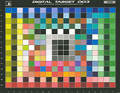 |
| The inexpensive 30-patch QPcard 201, which can be used with free downloadable QPcolorsoft 501 software for profiling cameras. Designed by Lars Kjellberg, founder of the outstanding lens test site, Photodo.com, which uses Imatest. The QPcard should be photographed in landscape mode with the Qpcard logo on the right. |
|
| The 140-patch X-Rite Colorchecker SG (Imatest Master only), which has a semigloss (SG) surface. It contains a 6x4 patch area in the upper-middle that is similar to the 24-patch Colorchecker, except that the colors are more saturated. |
|
| Linear grayscale step charts such as the Kodak Q-13/Q-14 (Imatest Master only) or the Stouffer T4110. Both reflection and transmission charts are supported. Available from most major photography dealers. Other stepcharts are discussed in Using Stepchart. |
|
| Special charts (Imatest Master only): Several additional monochrome charts as well as 7-12 squares, arranged on a circle, useful for analyzing pie or circular charts. Described on a separate page. |
|
| DSC Labs ChromaDuMonde 28/28R widely used in the cinema and broadcasting industries for calibrating cameras. Designed for use with the vectorscope display. Imatest Master can display vectorscope images from still frames. A future broadcast/cinema version will feature auto-refresh for full vectorscope functionality. |
|
A standard Windows dialog appears with the chart type indicated in the title. Open the image file.
If the image is the same size and type as the previous image analyzed by Multicharts, you'll be asked if you want to use the same ROI (region of interest).
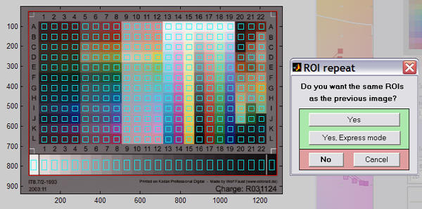
If the image is not the same size and type, or if you answer No, a coarse cropping box appears. The initial crop doesn't have to be precise: you'll have a chance to refine it shortly. The crop box can be enlarged or maximized to make the selection easier.
- For either of the ColorCheckers (24-patch or SG) or the QPcard, leave a margin around the sides slightly smaller than the spacing between patches.
- For Stepcharts, select the entire chart (all patches), choosing boundaries that give even patch size. (The white patch on the Q-13 and Q-14 is larger than the rest.)
- For IT8.7 charts, select an area that includes the boundaries around the color chart and the entire grayscale (the red rectangle in the fine adjustment box below).
If you selected a Stepchart, the box shown on the right appears. Select the chart type (which specifies the density step) and the number of patches (between 6 and 41). Kodak Q-13/Q-14 charts have 20 patches; the Stouffer T4110 (a transmission chart with a density range of 4.0) has 41. |
|
After you have made the rough crop, the fine adjustment box appears. The original crop is displayed as the red rectangle. The patch regions to be selected are the small cyan squares or rectangles. This dialog box can be enlarged or maximized to facilitate the adjustment. It offers numerous options.
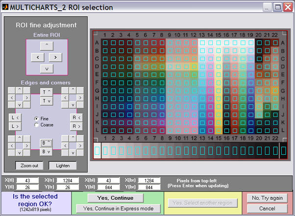
- The entire ROI can be moved ( ^ > v < , upper-left).
- The top, bottom, left, or right sides can be moved ( T^ Tv R> R< B^ Bv L> L< , middle-left).
- Corners can be moved individually (any of the 8 buttons in each of the four corners, middle-left).
- Pixel values for the four corners can be entered (X(tl), Y(br), ..., where tl = top-left, br = bottom right, etc.). The origin is the upper-left. Be sure to press the Enter key after entering a value.
- You can choose between Fine and Coarse movement (1 or 5 pixels of movement per click).
- The display can be zoomed out or in.
- The display can be lightened to view the dark regions more clearly.
- For some charts (those with relatively large patches) a Fill factor (linear) slider in the gray area above the No, Try again button specifies the relative size of the squares. Its default value is 0.5. Smaller values can be used where lens distortion or pattern alignment makes alignment difficult.
- The distortion slider allows highly distorted images (barrel or pincushion) to be analyzed.
When you have completed the fine adjustment, click one of the buttons on the bottom of the window. If you click Yes, Continue , an additional dialog box may appear. For example, for the IT8.7 chart it will ask for the required reference file. Some of the entries in the input dialog boxes, like color space, can be changed later. If you click Yes, Continue in Express mode , it will go directly to the Multicharts window, using saved (most recent) values. For example, it saves the IT8.7 reference file name.
Reference files
Several charts allow reference files to be entered. (IT8.7 and CMP DT003 charts require them.) The reference source can be entered in the Ref. box on the right of the Multicharts window, below the Color space box. The available settings depends on the chart type. The previous file is generally available. Here is a summary of the available reference sources.
X-Rite ColorChecker
(24-patch) |
Default values from GMB, BabelColor, or Danes Picta (a chart with the same geometry but different colors) or L*a*b*, xyY D50, or xyY D65 files in CSV format. |
| IT8.7 |
Requires a reference file in IT8.7 format, available from the chart manufacturer, generally available on their websites. |
| CMP DigitaL TargeT 003 |
Individually measured reference files are supplied with each target. |
| X-Rite ColorChecker SG |
Default values from GMB or user-supplied L*a*b*, xyY D50, or xyY D65 files in CSV format. |
| Stepchart (linear) |
Even density steps of 0.1, 0.15, 0.20, or 0.30 or an ASCII density reference file with one density value per line can be entered. The default is even density steps of 0.1. |
Except for the IT8.7 and CMP DT 003, reference files need to be in CSV (comma-separated file) format, which can be opened and edited in Excel. Color files (L*a*b*, xyY D50, and xyY D65) have three entries per line.
Here is an example of an L*a*b* file.
The format is CSV (comma-separated variables).
The format is the same for xyY files.
Spaces are for visual clarity (readability) only. |
55.261, -38.342,31.37
28.778, 14.179, -50.297
65.711, 18.13, 17.81
51.038, -28.631,-28.638
51.935, 49.986, -14.574
81.733, 4.039, 79.819
42.101, 53.378, 28.19 |
The Multicharts window
After the image file has been entered, the most recent Chart view is displayed. The 2D a*b* view (ideal and input values on the CIELAB a*b*) is shown below.
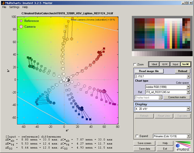
2D a*b* display of IT8 chart (CMYKRGB primaries)
The main display image is on the upper left. Color differences are summarized below this image, except when the Probe is turned on (available for the pseudocolor and split color displays). The various ΔE* and ΔC* values are described in Gamutvision equations. A synthesized image of the chart is shown on the upper right. Available options are described below. The remainder of the right side is the control area.
The Zoom checkbox turns Zoom on and off. 3D plots can be rotated when Zoom is turned off.
The four buttons to the right of Zoom control the display of the synthesized image on the upper-right.
- Ideal displays the ideal image with no gamut mapping. Colors will not be accurate for large gamut color spaces.
- Id>M displays the ideal image mapped from its native color space to sRGB, which is similar to typical monitor color spaces.
- Input displays the input image with no gamut mapping.
- In>M displays the input image mapped from its native color space to sRGB, which is similar to typical monitor color spaces.
|
IT8.7 chart
|
Image area
The pale blue box is the image area. It includes the Read image file and Reload buttons, the Chart type dropdown menu (described above), entries for image properties, and color correction matrix functions .
Reload reloads an image from a file or reacquires it from a device or video stream (depending on how the image was originally acquired). It is most valuable for versions of Imatest that can acquire images from devices or streams.
|
|
Color space allows the input file color space to be selected: the color space is not automatically read into Multicharts; it must be entered manually. One of six color spaces can be selected (more may be added in the future).
| sRGB |
The default space of Windows and the Internet. Limited color gamut based on typical CRT phosphors. Gamma = 2.2 (approximately), White point = 6500K (D65). |
| Adobe RGB (1998) |
Medium gamut, with stronger greens than sRGB. Often recommended for high quality printed output. Gamma = 2.2, White point = 6500K (D65). |
| Wide Gamut RGB |
Extremely wide gamut with primaries on the spectral locus at 450, 525, and 700 microns. One of the color spaces supported by the Canon DPP RAW converter. 48-bit color files are recommended with wide gamut spaces: banding can be a problem with 24-bit color. Gamma = 2.2, White point = 5000K (D50). |
| ProPhoto RGB |
Extremely wide gamut. Gamma = 1.8, White point = 5000K (D50). |
| Apple RGB |
Small gamut. Used by Apple. Gamma = 1.8, White point = 6500K (D65). |
| ColorMatch RGB |
Small gamut. Used by Apple. Gamma = 1.8, White point = 5000K (D50). |
Danny Pascale's A Review of RGB Color Spaces is recommended for readers interested in an in-depth explanation of color spaces.
Ref is the reference source for the ideal chart values. The contents of the popup menu depends on the chart type. For the 24-patch ColorChecker and the ColorChecker SG you can select either standard chart reference values or you can read in values from data files (Imatest Master only). Values for the two ColorCheckers have been supplied courtesy of X-Rite. You can select between six image file color spaces: sRGB, Adobe RGB (1998), Wide Gamut RGB, ProPhoto RGB, Apple RGB, or ColorMatch. Danny Pascale/Babelcolor's page on the ColorChecker contains nearly everything you want to know about the chart. Ian Lyons has a nice description of IT8.7 charts.
Correction matrix calculates the color correction matrix (Imatest Master only). After Correction matrix has been pressed it changes to Matrix calculated, highlighted with a pink background. The correction matrix cannot be recalculated until a property of the image changes (new image, color space, reference file, or color matrix setting). The Display input (or Corrected) dropdown menu, immediately to its left, is enabled. More details on using the color correction matrix can be found here.
Display selection box and area
The Display selection box allows you to select one of the following displays.
- Pseudocolor color difference. Shows the difference between the ideal and input color patches using any of several metrics. The pseudocolor scale is shown adjacent to the image (below, right). Probe is available for this display.
- 3D color difference.
- Split colors: ideal/input. Shows the patches split so that the ideal and input values are displayed in the upper left and the lower right or each patch region, respectively. Probe is available for this display.
- xy chromaticity.
- u'v' chromaticity.
|
|
- Black & White density.
- 3D L*a*b*. Shown on the right. L*a*b* coordinates can be difficult to visualize when viewed from a single angle. It needs to be rotated to be useful.
- EXIF data and Color matrix. Shows EXIF data if available and the color correction matrix if it has been calculated.
The Display area, immediately below the Display selection box, contains display options. The contents, which depend on the display selection, are described below in the sections for the individual displays.
Save screen (shown on the right) saves a snapshot of the current display (the entire Multicharts screen) as a PNG file (a widely-used losslessly compressed format). It also allows you to immediately view the snapshot so it can be used a reference for comparing with other results.
File name and Directory at the top of the window set the location of the file to save.
When you check the Open window in an image viewer... box, the current screen will be opened either the system default viewer (if the box under Image viewer is blank) or a viewer/editor of your choice (if the box contains the path name to the viewer/editor). I recommend using Irfanview, which is fast, compact, free, and supports an amazing number of image file formats. Its normal location in English language installations is C:\Program Files\IrfanView\i_view32.exe.
Save data Saves the key data in CSV and XML formats. This includes the input R, G, and B values, the input and reference L*, a*, b* values, and several of the color difference metrics.
Help opens this web page in an HTML browser window.
Exit terminates Imatest Multicharts, but the Imatest main window is still available.
Displays and options
Pseudocolor
Color difference
Shows the difference between the ideal and input color patches using any of several metrics using a pseudocolor color map. If a color correction matrix has been calculated, the difference between the ideal and corrected patches are shown at the bottom. The pseudocolor scale is shown adjacent to the image.
Probe (Checkbox; Pseudocolor and Split views) turns on the probe, illustrated below. When the probe is on, you can probe any patch in either image. The probe data (for the individual patch), shown below the split display, includes an image of the ideal and input patch colors, ideal and input RGB and L*a*b* values, and several ΔE* and ΔC* color difference metrics. (Corrected colors are used if a color correction matrix has been calculated and Display corrected has been selected.) |
Pseudocolor display for IT8.7 |
ΔE*ab, the geometric distance in L*a*b* space, is the most familiar, but ΔE*94, which is lower for chroma differences in highly chromatic colors (with large a*2 + b*2), may be a better measure of visual color difference. It's easy to correlate ΔE* metrics with visual color differences using this display. None of the metrics are perfect! The probe is turned off by clicking outside either of the images.
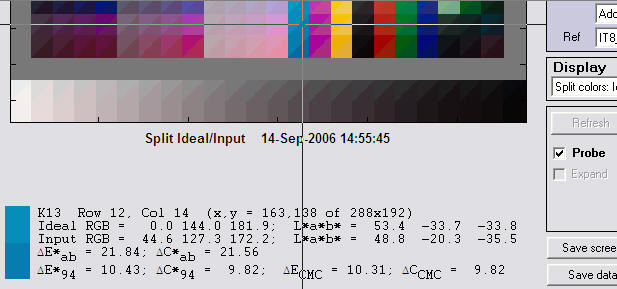
Split display for IT8.7 illustrating Probe
Color difference type (Popup menu to the right of the Probe checkbox; also in 3D Color difference) Contains a list of color metrics (mostly difference metrics) including ΔE*ab, ΔC*ab, ΔE*94, ΔC*94, ΔE00, ΔC00 (CIEDE2000 metrics that replaced ΔE*CMC and ΔC*CMC in Imatest 2.6.8), ΔL*, ΔChroma, Δ|Hue distance| , Δ(Hue angle) , Chroma (input) and Chroma (output).
Invert (Checkbox) inverts the color map. For the map shown (above, right), 0 would be black; maximum would be white.
Color map (Popup menu) allows you to select the color map. The WYRMBK color map shown goes from White - Yellow - Red - Magenta - Blue - Black.
3D
Color difference
Uses the height of the patches to display the difference between the ideal and input colors. Any of several metrics can be chosen. Can be zoomed and rotated. |
Light (Checkbox) Turns on light to highlight the shape of the plot. Default is On.
A-rotate (Toggle button; short for Auto rotate) starts rotating the image. Rotation is quite slow; it may be less useful than the 3D L*a*b* plot (below). The image continues to rotate until the next time you press the A-rotate button. It's best to turn off rotation before switching to other views.
Color difference type (Popup menu) Described above under Pseudocolor display.
Background (Slider) sets the background gray level.
Invert (Checkbox) inverts the up-down orientation of the 3D plot. |
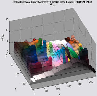 3D Color difference display for IT8.7
 |
Split colors
Displays a synthesized chart image with each patch split so the ideal value is in the upper left and the input (measured) value is in the lower right. If a color correction matrix has been calculated, corrected colors are shown at the bottom.
Probe (Checkbox) is the only option. Described above under Pseudocolor display. |
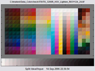
Split Color display for IT8.7 |
2D a*b*
Displays patch values on the CIELAB a*b* plane. Ideal values are displayed as squares; Input values are displayed as circles.
Expand (Checkbox; 2D a*b*, xy chromaticity, u'v' chromaticity, and 3D L*a*b*) Zoom in so the data fills the image. |
Region (Popup menu in the lower right of the Display area; also in xy chromaticity, u'v' chromaticity, and 3D L*a*b*) selects the region of the chart to display. For the IT8.7 and ColorChecker SG charts only. Avoids clutter from the large number of patches in these charts.
- For the IT8.7: Selections are Columns 1-4 (dark), 5-8 (middle), 9-12 (light), 13-19 (CMYKRGB primaries), and 20-22 (miscellaneous; unique to each chart manufacturer). Columns 13-19 are the most interesting.
- For the CMP DT 003: Selections are Saturated & Misc. ( a distribution of middle tones including the most saturated colors), Primary sequences (R, G, B,C, and Y for a range of lightnesses), and Pastels & skin tones.
- For the ColorChecker SG: Regions are less geometrically regular. Selections are 24-patch replica (middle), Pastels & skin tones, mid tones, and dark tones.
|
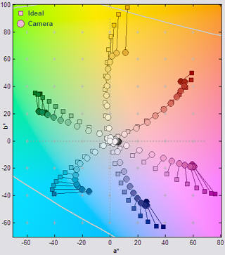
2D a*b* display for ITT8.7 |
xy and u'v' Chromaticity
Displays the xy and u'v' Chromaticity diagrams, which separate the visible and invisible color values into colored and gray regions. Ideal values are displayed as squares; Input values are displayed as circles. The u'v' Chromaticity diagram, which is more perceptually uniform than the more familiar xy diagram (shown in the Tour) is illustrated on the right. |
Wavelth (Checkbox) Turns the wavelength display (400-700 microns) on the periphery of the locus of visible colors on or off.
View (Popup menu to the right of Wavelth) selects between normal color (about as good a representation as is possible on a monitor) and lightened color (slightly easier to see the patch values).
Expand (Checkbox) Zoom in so the data fills the image.
Region (Popup menu in the lower right of the Display area) Described above under 2D a*b* display. |
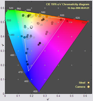
u'v' display for ColorChecker SG |
Black & White density
Shows the grayscale response curve. Available for all currently-supported color charts because all of them contain grayscale regions. |
Display type (Popup menu) allows you to select one of several B&W displays.
- Log pixels vs. input density. (shown on right) Gamma is the average slope for the lighter levels. The luminance (Y) channel is emphasized, but R, G, and B channels are also shown.
- Output vs. input density. The slope is ideally 1. Density is proportional to -Log10(Luminance).
- Output vs. input luminance. Shown on a linear scale.
- Output vs. input L* a* b* c*. Uses CIELAB values instead of density or (linear) luminance. Includes color values: a* (green-red), b* (blue -yellow), and c* (chrominance: (a*2 + b*2 )1/2 ).
|
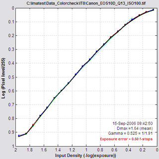
Log pixels vs. input density for Q-13 |
3D L*a*b*
Displays patch values in 3D CIELAB L*a*b* space with a wireframe representing the boundaries of the selected color space. Ideal values are displayed as squares; Input values are displayed as circles. Can be zoomed and rotated; you need to rotate it to be able to visualize patch locations. |
Wireframe properties (Popup menu) Turns wireframe on, off, or on with minimal (coarse) grid.
A-rotate (Toggle button; short for Auto rotate) starts rotating the image. This provides a better visual indication of the color locations. The image continues to rotate until the next time you press the A-rotate button. It's best to turn off rotation before switching to other views.
Transparency (Slider; default = 1) sets the wireframe transparency.Reducing transparency below 1 differentiates patches outside and inside the wireframe gamut boundary. Results are not reliable: patches near the boundary don't always appear as they should.
Background (Slider) sets the background gray level.
Region (Popup menu in the lower right of the Display area) Described above under 2D a*b* display.
Expand (Checkbox) Zoom in so the data fills the image. |
3D L*a*b* display for ColorChecker |
Vectorscope preview
The vectorscope duplicates the display in hardware vectorscopes, used for adjusting and calibrating broadcast and cinema cameras. It is designed to work optimally with the DSC Labs ChromaDuMonde 28 chart. (Other DSC charts will be added as customer demand warrants.)
There are several display options, including background color, reference and input display color. Llight input colors (circles) and dark reference colors (squares) are shown on a dark background. HDTV, SDTV, and NTSC/PAL vectorscope patterns can be displayed. The recommended color space for these signals is sRGB. At the present time the vectorscope omits the standard target rectangles because the RGBCMY primaries in the CDM chart are different from the standard color bars.
This image is a preview of a full-featured vectorscope function that will be included in an upcoming broadcast/cinema version of Imatest that continuously refreshes frames from a video stream using the Reload button instead of reading individual images from files. |
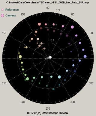
Vectorscope preview |
GretagMacbethTM and ColorChecker® are trademarks of X-Rite, Incorporated, which is not affiliated with Imatest. ColorChecker L*a*b* values are supplied courtesy of X-Rite.
Multicharts Special Charts
Additional charts, including circles arranged on a square
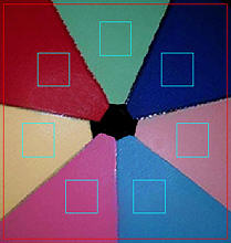
7-patch pie chart
|
Special Charts (a part of Multicharts, available with Imatest™ Pro) analyzes
- patterns consisting of 7 to 12 squares uniformly distributed around a circle, including portions of monochrome or color "pie" charts similar to the one shown on the left. These charts are useful for microscopy and for systems with significant light falloff (vignetting).
- any of the monochrome test charts shown below, which can also be analyzed by Stepchart. They are described in detail in Applied Image and ISO charts for Stepchart.
|
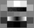
ISO-15739
Noise target |
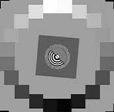
20-patch OECF
targets |
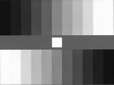
ITE Grayscale |
These illustrations show how the monochrome charts should be cropped.
Instructions
Photograph or scan the chart, taking care to avoid glare, which can be problematic with charts with semigloss and glossy surfaces, especially with wide angle lenses. A recommended lighting setup is described here and in the page on the Imatest testing lab.
|
To start Special Charts, run Imatest and click the Multicharts button on the left side of the Imatest window. The Multicharts window will appear with brief instructions.
Select Special Charts from the Read image file. Chart type: popup menu in the middle-right of the Multicharts window. The contents of this window is highlighted (brown text, yellow background) when Multicharts starts. |
A standard Windows file selection dialog appears, labelled Special Charts image file. Select an image file to open. You may, if you wish, press View ( ), Thumbnails to see thumbnails in the dialog box (illustrated on the right). This is sometimes helpful for locating the file to open. ), Thumbnails to see thumbnails in the dialog box (illustrated on the right). This is sometimes helpful for locating the file to open. |
 |
After the file is selected the Special Chart selection box appears. A thumbnail of the input image is shown on the right.
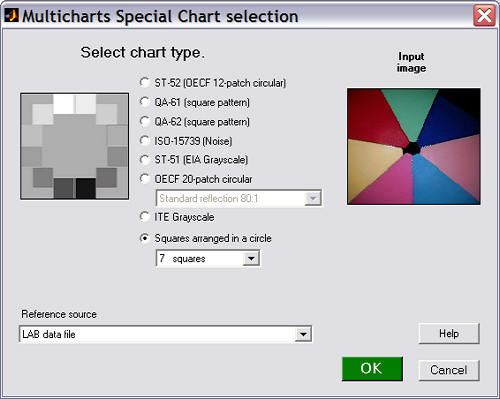
Select the chart type and the reference source. If an incorrect reference source is entered, it can be changed later in the Multicharts window. If you select Squares arranged in a circle, choose the number of squares in the pattern (7-12). If you choose OECF 20-patch circular, choose one of the following in the box below the OECF 20-patch radio button.
OECF 20-patch circular charts (more detail here) |
| TE 241 |
Available from Image Engineering/Esser Test Charts. Transmissive chart. 12600:1 contrast ratio. 0 ≤ density ≤ 4.1 |
| Low contrast 20:1 |
From ISO/DIS 14524, Table A3. 0.1 ≤ density ≤ 1.4 |
| Standard reflection 80:1 |
From ISO/DIS 14524, Table A3. 0.1 ≤ density ≤ 2.0 |
| Normal contrast 160:1 |
From ISO/DIS 14524, Table A3. 0.1 ≤ density ≤ 2.3 |
| High contrast 1000:1 |
From ISO/DIS 14524, Table A3. 0.1 ≤ density ≤ 3.1 |
If you choose ITE Grayscale, select either ITE Grayscale I: gamma = 0.45 or ITE Grayscale II: gamma = 1.0 in the box just above the ITE Grayscale radio button.
The reference source can be one of the following.
| Default reference values (if applicable) |
Available for the monochrome charts: ST-52, QA-61, QA=62, ISO-15739, EIA Grayscale. Not for Squares arranged in a circle. |
| Read from a density file |
For monochrome charts only. One value per line. a* = b* = 0. You will need to enter the file name. |
| Read from a L*a*b* file |
Three values per line (L*, a*, b*), separated by commas (CSV format). " " |
| Read from a 5000K xyY data file |
Three values per line (x, y, Y), separated by commas (CSV format). " " |
| Read from a 6500K xyY data file |
Three values per line (x, y, Y), separated by commas (CSV format). " " |
| Last file: (file name if applicable) |
The previous file name for this type of chart, if applicable. |
Here is an example of an L*a*b* file in
CSV (comma-separated variable) format.
The format is the same for xyY files.
Spaces are for visual clarity (readability) only.
The numbering order of the patches is shown below.
|
55.261, -38.342,31.37
28.778, 14.179, -50.297
65.711, 18.13, 17.81
51.038, -28.631,-28.638
51.935, 49.986, -14.574
81.733, 4.039, 79.819
42.101, 53.378, 28.19 |
Coarse crop box (greatly reduced)
If a reference file is called for, a dialog box for entering the file name will appear after the crop boxes. Details of required file contents are found in Numbering and orientation of the patches, below.
If the image is the same size and type as the previous image analyzed by Multicharts, you'll be asked if you want to use the same ROI (region of interest).
If the image is a different size or type, or if you answer No, a coarse crop box appears, shown greatly reduced on the right. Select a portion of the image, or click outside the image to select the entire image. Recommended cropping for the monochrome charts is shown near the top of the page. The initial crop doesn't have to be precise: you'll have a chance to refine the crop in the fine crop box. The crop box can be enlarged or maximized to make the selection easier.
|
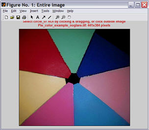
|
After you have made the rough crop, the fine adjustment box appears. The original crop is displayed as the red rectangle. The patch regions to be selected are the small cyan squares or rectangles. This dialog box can be enlarged or maximized to facilitate the adjustment. It offers numerous options.
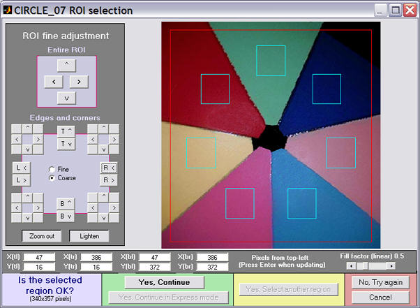
The original crop is displayed as the red rectangle. The patch regions to be selected are the small cyan squares or rectangles. This dialog box can be enlarged or maximized to facilitate the adjustment. Numerous options are available.Its numerous options are described in the Multicharts instructions. Fill factor (linear) allows the size of the squares to be adjusted.
- The entire ROI can be moved ( ^ > v < , upper-left).
- The top, bottom, left, or right sides can be moved ( T^ Tv R> R< B^ Bv L> L< , middle-left).
- Corners can be moved individually (any of the 8 buttons in each of the four corners, middle-left).
- Pixel values for the four corners can be entered (X(tl), Y(br), ..., where tl = top-left, br = bottom right, etc.). The origin is the upper-left. Be sure to press the Enter key after entering a value.
- You can choose between Fine and Coarse movement (1 or 5 pixels of movement per click).
- The display can be zoomed out or in.
- The display can be lightened to view the dark regions more clearly.
- The Fill factor (linear) slider in the gray area above the No, Try again button specifies the relative size of the squares. Its default value is 0.5. Smaller values can be used where lens distortion or pattern orientation makes alignment difficult.
When you have completed the fine adjustment, click one of the buttons on the bottom of the window. If you click Yes, Continue , an additional dialog box may appear. You may, for example, be asked for the required reference file. Some of the entries in the input dialog boxes, like Reference file, can be changed later. If you click Yes, Continue in Express mode , it will go directly to the Multicharts window, using saved values.
Numbering and orientation of the patches
The table below shows the patch order and orientation of supported charts.
Orientation and numbering of patches for squares arranged in a circle |
|
8 1
7 2
6 3
5 4
8 patches |
1
9
2
8
3
7 4
6 5
9 patches |
1
10 2
9 3
8 4
7 5
6
10 patches |
1
11 2
10 3
9
4
8
5
7 6
11 patches |
12 1
11 2
10 3
9 4
8 5
7 6
12 patches |
Pattern orientation rule: For n patches,
If n is odd or even and not a multiple of 4 (n = 7, 9, 10, or 11), patch 1 is centered at the top of the circle.
if n is a multiple of 4 (8, 12), patches 1 and n are side-by-side at the top, with patch 1 to the right of n.
Patches are numbered clockwise, starting at the top or just to the right of the top (for n a multiple of 4).
Patches for the monochrome charts below are numbered individually, following published descriptions or standards. There is no general rule.
Orientation and numbering of patches for monochrome targets |
1 2 3 4 5 6
20 7
19 8
18 9
17 10
16 15 14 13 12 11 |
1 2 3 4 5 6
20 7
19 8
18 9
17 10
16 15 14 13 12 11 |
1 2 3 4 5 6 7 8 9
10 11 12 13 14 15 16 17 18 |
1 2
3 4
5 6
7 8
9 10
11 12 |
QA-61 ISO-
16067-1 Scanner |
QA-62 |
ST-51
EIA Grayscale |
ST-52
ISO-14524
OECF target |
3 1 2
5 4
7 6
9 8
11 12 10 |
3 1 2 4
5 6
7 8
9 10
11 12
13 14
15 16
17 19 20 18 |
1 2 3 4 5 6 7 8 9 10 11
12 13 14 15 16 17 18 19 20 21 22 |
|
ISO-15739
Noise target
|
20-patch OECF targets |
ITE Grayscale |
|
Use these orders when creating reference files (density, L*a*b*, or xyY). These charts are described in more detail in Stepchart: Applied Image and ISO charts.
Examples of results
All Multicharts results are available in Special Charts, though not all results are usable. For example, the Black & White density produces jumbled plots for colored "pie" charts and many of the color displays display little useful information for monochrome charts.
The original chart is simulated (synthecially recreated) forall patterns except Squares arranged in a circle.
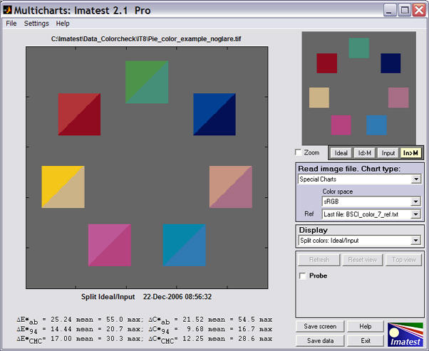
For squared arranged in a circle the selected squares are displayed on a gray background, even though the original is the "pie" chart illustrated above. Apart from that, Special charts displays are similar to Multicharts displays.
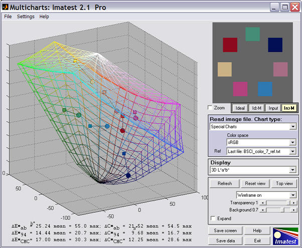
The 3D L*a*b* plot is typical. It can be rotated to faciliate visualization of color shifts.
Using Rescharts
Analysis of resolution-related charts
Introduction
Imatest™ Rescharts analyzes images of several test charts for resolution-related parameters such as sharpness (i.e., spatial frequency response; MTF), color moiré, and fine detail lost to software noise reduction, using a highly interactive user interface is similar to Multicharts.
The following chart types are supported by Rescharts.
Duplicates SFR, but with a far more interactive interface. It calculates and displays the average edge, SFR (Spatial Frequency Response or MTF), and Lateral Chromatic Aberration. Includes one figure not in SFR: a histogram with noise analysis.
It supports all charts that contain slanted edge patterns, including the ISO 12233 chart and its derivatives. Charts may be purchased from sources such as Applied Image or created with Test Charts (SVG charts are especially recommended) and printed on a high quality inkjet.
|
|
SFRplus
Highly automated analysis of SFR (MTF), Lateral Chromatic Aberration, distortion, and tonal response. Introduced in Imatest 3.2. Uses a special test chart, shown on the left. Unlike other Rescharts modules, SFRplus does not require manual region (ROI) selection: it is performed automatically. Running SFRplus in Rescharts saves settings for fully automated runs.
SFRplus instructions |
|
|
Log Frequency (simple)
Analyzes a sine or bar pattern of increasing spatial frequency. Measures SFR more directly, but less precisely, than the slanted-edge method. Also measures color moiré (Imatest Master only), which is a function of lens sharpness, anti-aliasing filter, and demosaicing algorithm. Spatial frequencies are detected automatically. Charts can be created by Test Charts and printed on a high quality inkjet printer. Also works with the old test chart in Lens testing.
Log Frequency instructions |
|
|
Log F-Contrast (Imatest Master only)
Analyzes a sine or bar pattern of increasing spatial frequency on the one axis and decreasing contrast on the other. Measures SFR for a range of contrast levels. Useful for measuring the loss of fine detail caused by software noise reduction— the effects of nonlinear signal processing. The chart can be created by Test Charts and printed on a high quality inkjet printer.
Log F-Contrast instructions |
|
|
Star chart (Imatest Master only)
Analyzes a sinusoidally-modulated Siemens star chart (144, 72, or 48 cycles); proposed for the revised ISO 12233 standard. Measures MTF (SFR) for 8, 12, or 24 segments around the circle. Has a large variety of displays. The chart can be purchased from Image Engineering or created by Test Charts and printed on a high quality inkjet printer.
Star Chart instructions |
Getting started
Instructions for purchasing or creating test charts can be found on pages for individual tests: SFR, Log Frequency, and Log F-Contrast.
Photograph or scan the chart, taking care to avoid glare, which can be problematic in charts with semigloss and glossy surfaces. Glare can be especially difficult to control with wide angle lenses. A recommended lighting setup is described here and in How to build a testing lab.
To start Rescharts, run Imatest, then click the Rescharts button. The Rescharts window will appear with brief instructions, which may be more up-to-date than the ones shown below.
Select an image to analyze by
- clicking on Read image file if the correct Chart type is displayed, or by
- clicking on one of the entries in the popup menu below Chart type:.
The Read image file button and Chart type popup menu are highlighted (yellow background) when Rescharts starts. |
|
A standard Windows dialog appears with the chart type indicated in the title. Open the image file. Multiple files can be opened for averaging (but batch (sequential) runs are not supported by Rescharts).
If the folder contains meaningless camera-generated file names such as IMG_3734.jpg, IMG_3735.jpg, etc., you can change them to meaningful names that include focal length, aperture, etc., with the View/Rename Files utility, which takes advantage of EXIF data stored in each file.
For all modules other than SFRplus, if the image is the same size and type as the previous image analyzed by Rescharts, you'll be asked if you want to use the same ROI (region of interest). (ROI selection is entirely automatic with SFRplus.)
If the image size or type is different or if you answer No, a coarse cropping box appears. The initial crop doesn't have to be precise: you'll have a chance to refine it.
- For Slanted-Edge SFR, select the region you want. Recommended cropping.
- For Log Frequency (simple), select a narrow strip running from along the direction of increasing spatial frequency. Narrow strips of the Log Frequency-Contrast chart can be used.
- For Log F-Contrast, select most of the chart image, leaving small margins (1/2 to 1% of the image dimensions) at the edges.
After the rough crop has been selected, the fine adjustment box appears, showing the coarse crop as a rectangle. This dialog box can be enlarged or maximized to facilitate the adjustment. It offers numerous options.
Crop for the Log Frequency-contrast chart. Leave a small margin
(1/2 - 1% of the image height) at the top and bottom.
- The entire ROI can be moved ( ^ > v < , upper-left).
- The top, bottom, left, or right sides can be moved ( T^ Tv R> R< B^ Bv L> L< , middle-left).
- You can choose between Fine, Coarse, and Extra Coarse movement (1, 5, or 25 pixels of movement per click).
- The display can be zoomed out or in.
- Pixel values for the four corners can be entered (X(tl), Y(br), ..., where tl = top-left, br = bottom right, etc.). The origin is the upper-left. Be sure to press the Enter key after entering a value.
When you have completed the fine adjustment, click one of the buttons on the bottom of the window. If you click Yes, Continue , an additional dialog box may appear. The entries in this dialog box can be changed later by clicking on Image settings & options in the Rescharts window. If you click Yes, Continue in Express mode , it will go directly to the Rescharts window, using saved (recent) values.
The Rescharts window
After the image file has been entered, calculations are performed and the most recent Chart view is displayed. The MTF/contrast (2D pseudocolor contour) display (actual MTF when a sine chart is used) for Log F-Contrast is shown below.
MTF contours for Canon EOS-20D, 24-70mm f/2.8L, 42mm, f/5.6, ISO 100
The main display image is on the upper left. Additional text results may appear below this image. An image of the chart is shown on the upper right. You can choose to display the whole image or the crop (ROI). The remainder of the right side is the control area.
The Zoom checkbox turns Zoom on and off.
The buttons to the right of Zoom set the display to either the Whole image or a Crop of the image (the selected ROI).
Image and Display areas
The image area is on the right of the Rescharts window, just below the Whole image and Crop buttons. It includes the the Read image file and Reload buttons, the Chart type dropdown menu (described above), and additional controls.
Reload reloads an image from a file or reacquires it from a device or video stream (depending on how the image was originally acquired). It is most valuable for versions of Imatest that can acquire images from devices or streams.
Immediately below the Chart type menu is the New crop (same image) menu, which has identical entries. If an item is selected on this menu, the image is recropped for analysis by the selected chart type (which may be the same or different). This menu is useful when several regions of an image need to be analyzed or when the target contains more than one chart type.
Image settings & options brings up the input dialog box for the selected chart type. This is the same box that appears when you press Yes, continue (not Express mode) in the ROI repeat or ROI selection window.
Display, immediately below the image area, selects the results to display. Choices depend on the chart type.
|
|
The Display options area is immediately below Display. The contents, which depend on the Display selection, are described below in the sections for the individual displays.
Save screen (shown on the right) saves a snapshot of the current display (the entire Rescharts screen) as a PNG file (a widely-used losslessly-compressed format). It also allows you to immediately view the snapshot (if the Open window... box is checked) so it can be used a reference for comparing with other results.
File name and Directory at the top of the window set the location of the file to save.
When you check the Open window in an image viewer... box, the current screen will be opened either the system default viewer (if the box under Image viewer is blank) or a viewer/editor of your choice (if the box contains the path name to the viewer/editor). I recommend Irfanview, which is fast, compact, free, and supports an amazing number of image file formats. (It can be valuable for converting nonstandard images to Imatest-readable formats.) Its normal location in English language installations is C:\Program Files\IrfanView\i_view32.exe. |
|
Save data Saves detailed results in CSV and XML formats. The exact content depends on the module.
Help opens this web page in an HTML browser window.
Exit terminates Imatest Rescharts, but the Imatest main window remains available.
Rescharts modules
This section describes the Rescharts modules, illustrating some of the available displays and options. More information is available in the pages for the individual modules (Chart type analyses).
Slanted-edge SFR
Slanted-edge SFR measures sharpness as Spatial Frequency Response, also called MTF (Modulation Transfer Function) from images of slanted edges, as described in Sharpness. ROI (Region of Interest) selection, calculations, and output largely duplicate SFR. Available displays:
| Edge and MTF (shown on the right) |
| Chromatic Aberration (right, below) |
| SQF (Subjective Quality Factor) |
| Noise spectrum & Shannon capacity |
| Histograms & noise stats (left, below) |
| Summary & EXIF (for JPEGs) |
The principal differences from SFR are the highly interactive interface and an added histogram of the ROI levels, shown below. Black is the entire ROI. Cyan is the portion on the left and red is the portion on the right, both away from the edge. The upper histogram is for the original image (pixel levels/255); the lower histogram is for the linearized image (gamma applied). |
SFR Edge and MTF display
|
SFR Histogram |
SFR Lateral Chromatic Aberration |
SFRplus
| SFRplus, introduced in Imatest 3.2, performs a highly automated analysis of SFR (MTF), lateral chromatic aberration, distortion, and tonal response, using a special test chart. Unlike other Rescharts modules, SFRplus does not require manual region (ROI) selection: it is performed automatically. Running SFRplus in Rescharts saves settings for fully automated runs. |
| Edge and MTF |
| Chromatic Aberration |
| SQF |
| Noise spectrum & Shannon capacity |
| Multi-ROI summary |
| Tonal response & gamma |
| Histograms and noise stats |
| Summary & EXIF (for JPEGs) |
|
SFRplus summary display for 9 automatically-selected regions
Log Frequency (simple)
Log frequency image: right-click to download an image that can be used for testing.
Log Frequency measures image contrast of charts that increase in spatial frequency on a logarithmic scale (log frequency increases with x). When the image pattern is sinusoidal (not a bar pattern) the contrast is equivalent to SFR or MTF. This method is more direct than Slanted-edge SFR, but less accurate because it is degraded by noise and sampling phase variation. It also measures color moiré (Imatest Master only). The chart can be created by Test Charts and printed on a high quality inkjet. Also works with the test chart in Lens testing and narrow strips of the Log Frequency-Contrast chart..
Available displays: Full instructions
| The Pattern (original pixel levels and linearized) |
| MTF and Moire (linear frequency scale) |
| MTF and Moire (log frequency scale) |
| EXIF data |
The display on the right shows Contrast (MTF) on the top and color moire on the bottom as a function of spatial frequency (displayed linearly). Color moire can me measured in several ways: R-B (normalized Red − Blue channel) is shown on the right. The total color moire is the spread of values above 0.3 cycles/pixels (indicated by the red curve). Details of the color moire measurement can be found in Log Frequency. The Correct for color density box should be checked for best results.
Pattern (original pixel levels and linearized)
|
Log Frequency MTF and moire display
(linear x-axis frequency scale) |
Log F-Contrast
Log F-Contrast (short for Log Frequency-Contrast) measures the image contrast of charts that vary in spatial frequency on one axis (log frequency increases with x) and in contrast on the other (contrast is proportional to ( y/h)2 for image height h). When the image pattern is sinusoidal (rather than a bar pattern) the contrast is equivalent to SFR or MTF. This module can be used to measure how much fine, low-contrast detail is lost to software noise reduction. The chart can be created by Test Charts and printed on a high quality inkjet printer.
Available displays: Full instructions
| The Pattern (original pixel levels and linearized) |
| MTF (linear frequency scale) |
| MTF (log frequency scale) |
|
2D pseudocolor contour plots that can display any of several MTF-related parameters: |
MTF (envelope - standard) (standard MTF, normalized to 1 at maximum contrast and zero spatial frequency) |
Normalized contrast level (MTF normalized to 1 at zero spatial frequency for all contrast levels) |
Normalized contrast loss (MTF normalized to 1 at zero spatial frequency for all contrast levels as well as all spatial frequencies at the maximum contrast level: shows contrast loss from ideal) |
| MTFnn or MTFnnP (spatial frequencies where MTF = nn% of the low frequency or peak value |
| EXIF data |
The displays on the right show the Normalized contrast level (MTF normalized to 1 at low spatial frequencies for all chart contrast levels) for the Panasonic TZ1 camera with ISO speed set at 80 (top) and 800 (bottom). Spatial frequency is on a linear scale with a maximum displayed frequency of 0.5 cycles/pixel. The difference between the two images is quite striking. The TZ1 has much more noise reduction— and correspondingly less detail— at ISO 800. These plots are explained in detail in Log F-contrast. |
Normalized contrast level (MTF)
(1 at low frequencies
for all chart contrasts):
Panasonic TZ1, ISO 80
Normalized contrast level: TZ1, ISO 800 |
Star chart
Star Chart measures contrast (MTF or SFR) of sinusoidally-modulated star charts (also known as the Siemens star) proposed for inclusion in the updated ISO 12233 standard. Charts have 144, 72, or 48 cycles and can be analyzed in 8, 12, or 24 segments. Star charts can be purchased from Image Engineering or created by Test Charts and printed on a high quality inkjet printer.
Available displays: Full instructions
| Display |
Description |
| MTF (original and linearized) |
MTF for up to 8 segments of the star. Both linear and logarithmic frequency displays are available. |
| MTFnn or MTFnnP |
Display MTFnn (the frequencies where MTF equals nn % of the low frequency values) and MTFnnP (the frequencies where MTF equals nn % of the peak value) for nn = 70, 50, 30, 20, and 10. Both polar (spider) and rectangular plots are available. |
| MTF contours (rectangular) |
Display MTF contours in a rectangular plot with linear or logarithmic frequency display. Similar to the MTFnn rectangular plot. |
| MTF contours (polar) |
Display MTF contours in a polar plot whose geometry duplicates that of the target. |
| EXIF data |
Show EXIF data if available. |
The displays on the right show MTF contours and MTF70 through MTF10 (spatial frequencies where MTF = 70 through 10% of the low frequency level). Spatial frequency is displayed in cycles per pixel, but Line Widths per Picture Height (LW/PH), cycles/inch, or cycles/mm can be selected by pressing Image settings & options. |
MTF contours, rectangular display,
Linear frequency scale.
MTF70 – MTF10: Polar coordinates,
Linear frequency on radius. |
Log Frequency
Analysis of log frequency-varying charts
Introduction
Log frequency, which uses the Rescharts interface, measures the contrast of narrow bar or sine charts that increase logarithmically in spatial frequency. It also measures color moiré (Imatest Master only). When the image pattern is sinusoidal (rather than a bar chart), contrast is equivalent to SFR or MTF. This method is more direct than the slanted-edge method, but less accurate and more susceptible to noise. A chart can be created by Test Charts and printed on a high quality inkjet printer.
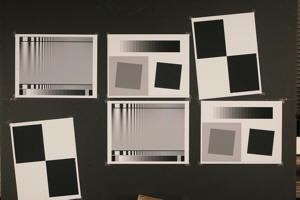

Log Frequency image (complete and cropped)
The image above used to illustrate the Log frequency module and to compare results with Slanted-edge SFR. It was captured with a Canon EOS-20D camera, 24-70mm f/2.8L lens set at 42mm, f/5.6, ISO 100. It includes Log Frequency-Contrast charts and slanted-edges with high and low contrast (20:1 and 2:1). Log frequency was run using a narrow strip of the Log f-contrast chart, as shown above.
Creating and photographing the chart and running the program
Create the test chart, which may not be commercially available, using Imatest Test Charts, then print the chart on a high quality inkjet printer. Test Charts has a number of options. The dialog box and recommended settings are shown in Log F-Contrast. In Imatest Studio, Type (bar or sine) should be set to Bar, sine (4x).
Mount the chart on a flat dark board— 1/2 inch foam board works well; thinner board warps more easily. Depending on the number of horizontal pixels in the chart to be analyzed, the chart should occupy 1/3 to 1/4 of the horizontal frame. Other charts can be mounted along with it.
Orientation. The pattern may be rotated by multiples of 90 degrees from the orientation shown: it may be have portrait as well as landscape orientation.
Photograph the chart using the sort of lighting described in Imatest Lab or How to test lenses, taking care to avoid glare. Save the image in any one of several high quality formats, but beware of JPEGs with high compression (low quality), which will show degraded quality, unless, of course, you are testing JPEG degradations. (Unlike the slanted-edge, the Log f-contrast pattern reveals JPEG losses quite clearly).
Open Imatest, then click on Rescharts. The Rescharts window is described in the Rescharts page.
Select a pattern to analyze (in this case, Log frequency (simple) ) by clicking on one of the entries in the popup menu below Chart type or by clicking on Read image file if Log frequency (simple) is displayed. The Read image file button and popup menu (shown on the right) are highlighted (yellow background) when Rescharts starts. |
|
Select the image to read. If the pixel size is the same as the previous Log frequency run, you'll be asked if you want to use the previous ROI, adjust the previous ROI, or crop anew. If the folder contains meaningless camera-generated file names such as IMG_3734.jpg, IMG_3735.jpg, etc., you can change them to meaningful names that include focal length, aperture, etc., with the View/Rename Files utility, which takes advantage of EXIF data stored in each file.
Cropping The pattern should be cropped to a narrow strip, as shown in the ROI fine adjustment window, below. 10 to 25 pixels is a typical strip width, though more pixels may work if the chart is well-aligned. The ROI fine adjustment window may be maximized to facilitate fine selection.
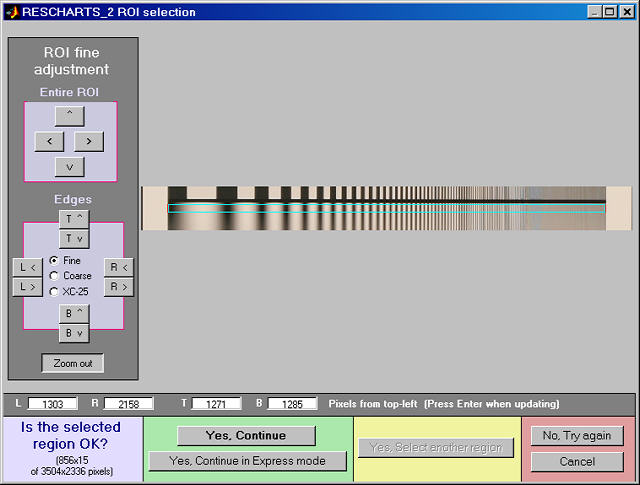
ROI fine adjustment window showing the Log Frequency-Contrast image
cropped
for use with Log frequency (simple). Canon EOS-20D camera,
24-70mm f/2.8L lens
set at 42mm, f/5.6, ISO 100.
Click on image to load full-size image.
If Express mode is not selected, the input dialog box shown on the right appears. Since this dialog box is used for several modules, some entries such as SQF options are not relevant.
Settings
Gamma is used to linearize the test chart. It can be measured by Stepchart, Colorcheck, or Multicharts. 0.5 is a typical value for color spaces intended for display at gamma = 2 2 (sRGB, Adobe RGB, etc.).
Channel is R, G, B, or Y (luminance; the default).
Color space is used only for the color moiré L*a*b* chroma plot (sqrt(a*2 + b*2)).
Display options
MTF plots selects the x-axis scaling. If Cycles/inch or Cycles/mm are selected, the pixel spacing (um/pixel, pixels/inch, or pixels/mm) should be entered.
X-axis scaling for linear plots selects the maximum spatial frequency to be displayed.
|
 |
Don't worry about getting all settings correct: You can always open this dialog box by clicking on Image settings & options in the Rescharts window.
After you press OK, calculations are performed and the most recently-selected display appears.
Color moiré
Color moiré is artificial color banding that can appear in images with repetitive patterns of high spatial frequencies, like fabrics or picket fences. The example on the right is a detail of a shirt captured by the Canon Rebel XT with its excellent kit lens.
Color moiré is the result of aliasing in image sensors that employ Bayer color filter arrays, as explained below. Key points:
- Color moiré can appear when there is significant image energy above the sensor Nyquist frequency for the red and green channels (0.25 cycles/pixel; half the image Nyquist frequency of 0.5 cycles/pixel).
- It is affected by lens sharpness, the anti-aliasing (lowpass) filter (which softens the image), and demosaicing software. It tends to be worst with the sharpest lenses.
- It is most noticeable in the red and blue channels.
- Color moiré should be measured near the center of the image, where lenses tend to be sharpest and lateral chromatic aberration (which can mimic color moiré) is minimal.
|
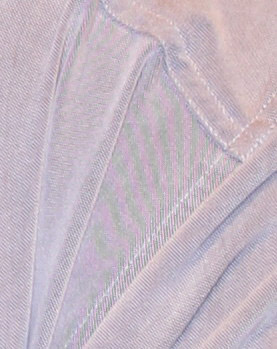
Color moiré on fabric
(Canon Rebel XT with kit lens)
|
Since there is no well-established standard for measuring color moiré (to the best of our knowledge), we have added a highly versatile measurement to Log Frequency in Imatest Master. One of the parameters shown on the right, selected by the Moire box in the Plot settings area of the Rescharts window, is plotted immediately below MTF in the MTF & Moire displays. The two parameters shown in boldface, R-B and L*a*b* chroma (sqrt(a*2+b*2 )) have proven to be the most useful. A color moiré plot is shown below.
The Correct for color density checkbox, which corrects for tonal imbalances in the image, should normally be checked. The lowest frequency where moiré can be visible with Bayer sensors is 0.25 cycles/pixel, half the image Nyquist frequency. This is so because the sensor pixel spacing for the red and blue channels is twice that of the (final demosaiced) image pixel spacing. The total moiré for a selected parameter is the variation of that parameter above 0.3 cycles/pixel, shown in bold red in the plot. For the plot below, it is the maximum − minimum L*a*b* chroma (√(a*2+b*2 )) above 0.3 c/p = 14.9 (L*a*b* units).
|
| R-B |
The most useful of the color differences |
| (R-B)/(R+B) |
|
| R-G |
|
| (R-G)/(R+G) |
|
| G-B |
|
| (G-B)/(G+B) |
|
| S(HSL) |
Saturation in HSL color |
| S(HSV) |
Saturation in HSV color |
| Chroma (sqrt(a*2 + b*2)) |
Chroma in L*a*b* space |
Color moiré measurements |
|
Log Frequency pattern with exaggerated chroma |
|
Color moire results expressed as L*a*b* chroma |
Output
The Display box in the Rescharts window, shown below, allows you to select any of several displays. Display options are set in boxes that appear below Display. All displays except Exif data have a channel selection option (Red, Green, Blue, or Luminance (Y) (0.3R + 0.59G + 0.11B).
| Display |
Description |
| Pattern (original and linearized) |
Show pattern: normalized pixel levels (max contrast) on top; linearized (max contrast and selected row) on bottom |
| MTF & Moire (Linear frequency scale) |
Display MTF for several contrast levels (rows 1-22 in steps of 3, where the chart is divided into 25 rows for analysis) with a linear frequency scale. |
| MTF & Moire (log frequency scale) |
Display MTF for several contrast levels (rows 1-22 in steps of 3) with a log frequency scale. A thumbnail of the pattern is also displayed on the same scale. |
| EXIF data |
Show EXIF data if available. |
In addition to the displays, two buttons allow you to save results. |
| Save screen |
Saves an image of the Starchart window as a PNG file. If you check Display screen in the Save screen dialog box, the image will be opened in the editor/viewer of your choice. (Irfanview works well, and it's free.) |
| Save data |
Saves detailed results in a CSV file that can be opened by Excel and also in an XML file. |
The spatial frequency is automatically calculated from the image, under the assumption that log frequency increases linearly with distance.
Pattern (original and linearized)
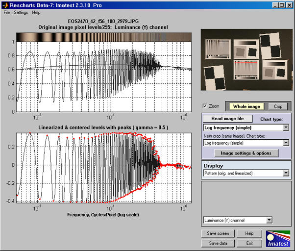
Pattern: original and linearized
The entire Rescharts window is shown. The upper plot is the normalized pixel level (pixel level/255 for bit depth of 8). The lower plot is the linearized levels.
MTF
The display on the right shows MTF on a logarithmic frequency scale. A vertically squeezed version of the image with exaggerated color (chroma) is shown just above the plot.
The dark line had been strongly smoothed. The pale dashed lines are the unsmoothed results: the fine detail is a calculation artifact caused by phase variations and noise; it is not significant.
The lower plot shows color moiré (in Imatest Master only) , which is discussed above. The selected moiré measurement is the Red-Blue channel (R-B). Options that affect this plot include Moire (the moiré measurement) and Correct for color density (which is normally checked).
The printed results beneath the plot shows
- the image dimensions and crop locations,
- MTFnn and MTFnnP (the spatial frequencies where response falls to nn% of the low frequency and peak values, respectively) for nn = 50, 20, and 10%, and
- The total moiré spread, which is the maximum - minimum value of the selected moiré measurement (in this case, R-B).
|
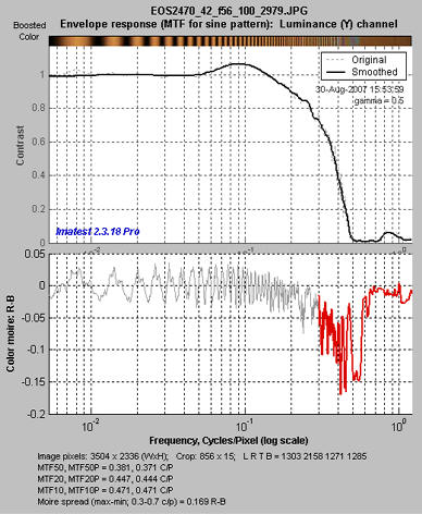
MTF: Log frequency scale
|
The display on the right shows the same MTF results plotted on a linear frequency scale with a maximum spatial frequency of 1 cycle/pixel. (Color moiré has been omitted.)
The maximum display frequency, the display scale (cycles/pixel, cycles/mm, cycles/in, or LW/PH (Line Widths per Picture Height, where 2 Line Widths = 1 cycle or line pair)), and gamma can be set to any of several options by pressing the Image settings & options button. |
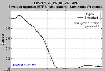
MTF: Linear frequency scale |
Comparison with other measurements
An obvious question is, how do Log Frequency results compare with Slanted-edge SFR (identical to the standard SFR module)? The comparison is easy to make because the test target contains low and high contrast slanted-edge charts as well as Log Frequency-Contrast charts.
Some divergence is expected because of nonlinear signal processing, which is widespread in digital cameras: most digital cameras, especially compacts, process the signal differently in the presence or absence of contrasty edges. In the presence of a contrasty edge the image is sharpened: high spatial frequencies are boosted. In the absence of a contrasty edge noise reduction is applied, i.e., the image is blurred; high spatial frequencies are attenuated. Since the Log Frequency pattern doesn't resemble an edge it's difficult to predict exactly how the different methods will compare.
But we have a clue from Log F-Contrast. The MTFnn values for the EOS-20D at ISO 100 (shown on the right) change relatively little with chart contrast, in strong distinction to the compact Panasonic TZ1, especially at ISO 800, which shows considerable nonlinear processing. |
MTFnn from Log F-Contrast:
shows little change with chart contrast
|
The low contrast (2:1) slanted-edge MTF is shown on the right. Although its shape is slightly different from the Log Frequency results (see MTF with linear frequency scale, above), MTFnn results are remarkably close: MTF50 is 0.347 vs. 0.381 c/p; MTF20 is 0.425 vs. is 0.444 c/p. The high contrast edge, below right, has similar MTF50 but much higher MTF20.
There are several reasons why the different charts may give different results. In all cases the slanted-edge measurement are more accurate, though of course it represents MTF at edges and not in the presence of gradually-varying features.
- Nonlinear signal processing can a major cause of differences, though the MTFnn plot for the EOS-20D as ISO 100, above right, indicates relatively little nonlinear processing.
- Noise can cause errors in the Log Frequency results. It is averaged out in the slanted-edge algorithm.
- Sampling phase errors can reduce the measured Log Frequency MTF above about 0.25 cycles/pixel. Second-order interpolation is used to detect peak amplitudes between 0.06 and 0.5 cycles/pixel, but above about 0.25 cycles/pixel (half-Nyquist frequency) it becomes increasingly ineffective at recovering peak values. The sampled value is often lower than the peak value, reducing the measured MTF.
- Alignment. If the chart is tilted, high frequency MTF response will be reduced.
Despite these factors, a reasonable match between the different methods can be obtained if nonlinear signal processing is not strong. |
MTF from low-contrast (2:1) slanted edge
|
 MTF from high-contrast (20:1) slanted edge
 |
Some calculation details
Second-order interpolation, illustrated below, is used in detecting peaks at spatial frequencies between 0.06 and 0.5 cycles/pixel It increases the peak amplitude for detected peaks between sampling points.. At lower frequencies it does little to improve accuracy because the signal varies slowly. It also has no benefit above the Nyquist frequency (0,5 cycles/pixel), where the signal consists of noise and aliasing. The red dots in the illustration show the peak amplitudes corrected with second order interpolation (with uncorrected peak locations).
The peak and its two adjacent points are assumed to fit the equation, y = ax2 + bx + c. The actual peak location is xp = -b/2a (x2 is shown in the above plot). The peak amplitude is ap = b2/2a + c.
Smoothing. The MTF & Moiré displays contain two curves: unsmoothed (thin dashed lines) and smoothed (thick solid lines). The smoothed curves are emphasized because the roughness in the unsmoothed curves is entirely an artifact of the calculations, resulting from sampling phase and noise— irregularities can result from noise on a single peak. Irregularities are reduced, but not eliminated, by second-order interpolation. It is important to realize that the features of the unsmoothed curve have no physical meaning.
The Nyquist sampling theorem, aliasing, and color moiré
(This section was adapted from normankoren.com.)
The Nyquist sampling theorem states that if a signal is sampled at a rate dscan and is strictly band-limited at a cutoff frequency fC no higher than dscan/2, the original analog signal can be exactly reconstructed. The frequency fN = dscan/2 is called the Nyquist frequency. By definition fN is always 0.5 cycles/pixel.
The first sensor null (the frequency where a complete cycle of the signal covers one sample, hence must be zero regardless of phase) is twice the Nyquist frequency. The sensor's average sensitivity (the average of all sampling phases) at the Nyquist frequency can be quite large.
Signal energy above fN is aliased— it appears as artificially low frequency signals in repetitive patterns, typically visible as moiré patterns. In non-repetitive patterns aliasing appears as jagged diagonal lines— "the jaggies" (a less severe form of image degradation). The figure below illustrates how response above the Nyquist frequency leads to aliasing.
|
Example of aliasing
|
| Signal (3fN /2) |
|
|
|
|
|
|
|
|
|
|
|
|
|
|
|
|
|
|
|
|
|
|
|
|
| Sensor pixels |
|
1 |
|
|
2 |
|
|
3 |
|
|
4 |
|
|
5 |
|
|
6 |
|
|
7 |
|
|
8 |
|
| Response ( fN /2) |
|
|
|
|
|
|
|
|
|
|
|
|
|
|
|
|
|
|
|
|
|
|
|
|
|
In this simplified example, sensor pixels are shown as alternating pink and cyan zones in the middle row. By definition the Nyquist frequency is 1 cycle in 2 pixels = 0.5 cycles/pixel. The signal (top row; 3 cycles in 4 pixels) is 3/2 the Nyquist frequency, but the sensor response (bottom row) is half the Nyquist frequency (1 cycle in 4 pixels)— the wrong frequency. It is aliased.
The sensor responds to signals above Nyquist— MTF is nonzero, but because of aliasing, it is not good response.
In digital cameras with Bayer color filter arrays— sensors covered with alternating rows of RGRGRG and GBGBGB filters— the problem is compounded because the spacing between pixels of like color is significantly larger than the spacing between pixels in the final image, especially for the Red and Blue channels, where the Nyquist frequency is half that of the final image. This can result in color moiré, which can be highly visible in repetitive patterns such as fabrics. Demosaicing programs (programs that fill in the missing colors in the raw image) use sophisticated algorithms to infer missing detail in each color from detail in the other colors. These algorithms can have a significant effect on color moiré. |
Bayer CFA
|
Many digital camera sensors have anti-aliasing or lowpass filters to reduce response above Nyquist. Anti-aliasing filters blur the image slightly, i.e., they reduce resolution. Sharp cutoff filters don't exist in optics as they do in electronics, so some residual aliasing remains, especially with very sharp lenses. The design of anti-aliasing filters involves a tradeoff between sharpness and aliasing (with cost thrown in).
Extreme aliasing. The now-discontinued 14-megapixel Kodak DCS 14n, Pro N, and Pro C, had no anti-aliasing filter. With sharp lenses, MTF response extended well beyond the Nyquist frequency. The 14n behaved very badly in the vicinity of Nyquist (63 lp/mm), as shown in this MTF test chart image, supplied by Sergio Lovisolo. This is about as bad as it gets. |
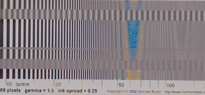 |
The Foveon sensor used in Sigma DSLRs is sensitive to all three colors at each pixel site. It also has no anti-aliasing filter and high MTF at Nyquist, but aliasing is far less visible because it is monochrome, not color. |
Log F-Contrast
Analysis of charts that vary in log frequency and contrast
Introduction
Log F-Contrast (short for Log Frequency-Contrast; Imatest Master only), which uses the Rescharts interface, measures the image contrast of charts that vary in spatial frequency on one axis (log frequency increases with x) and in contrast on the other (contrast is proportional to ( y/h)2 for image height h). When the image pattern is sinusoidal (rather than a bar pattern) the contrast is equivalent to SFR or MTF.
This module can be used to measure fine, low-contrast detail lost to software noise reduction, which can result in a "plastic" appearance in areas where fine texture is missing. This type of nonlinear signal processing is especially common in cameras with tiny pixels (< 2 microns), such as cameraphones. The chart can be created by Test Charts and printed on a high quality inkjet printer. An image of a Log Frequency-Contrast chart, acquired with a Canon EOS-20D camera, is shown below, slightly reduced.
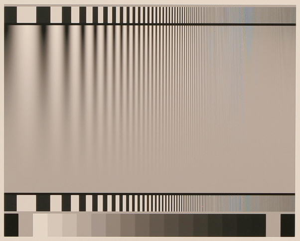
Log F-Contrast Image, Canon EOS-20D camera, 24-70mm f/2.8L lens
set at 42mm, f/5.6, ISO 100.
Click on image to load full-size image.
The chart is divided into twenty-five zones (numbered from top to bottom) for analyzing contrast (MTF), which can be displayed in several ways. Second-order interpolation and smoothing are used to increase the accuracy of the MTF calculations. Spatial frequency is derived from the pattern.
Creating and printing the chart
Since the Log Frequency-contrast chart is not (to our knowledge) commercially available, you will need to download it or create it using Imatest Test Charts and print it on a high quality inkjet printer. (Imatest LLC can supply high quality charts on request. Contact us for details.)
Downloadable charts
Two Log F-Contrast sine charts are available as PNG files (around 0.8 MB) for download and printing on high quality inkjet printers. One is optimized for printing at 600 dpi on HP and Canon printers; the other is for 720 dpi on Epson printers. Both are designed to be printed 20 cm (7.874 inches) wide (20 cm high if printed in landscape mode) on letter size or A4 paper using high quality print settings.
600 dpi 20 cm chart | 720 dpi 20 cm chart (Right-click to download.)
Both charts have a frequency ratio of 200:1 and a maximum frequency of 800 cycles/width. They should work well covering roughly 1/3 of the image width of typical digital cameras, as shown in the example below. |
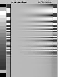 |
Test Charts has a number of options. The dialog box and recommended settings are shown below.
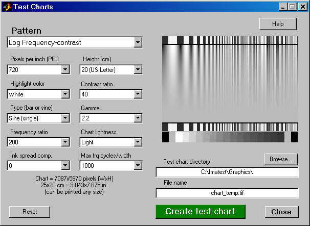
| Box |
Recommended setting |
| Pattern |
Log Frequency-contrast. |
| Pixels pre inch (PPI) |
Depends on printer. For best results set to 720 (Epson) or 600 (HP, Canon) and print at the indicated Height. |
| Height |
Print height (refers to landscape orientation). To get the indicated PPI— for best print quality— the image should be printed at this height. |
| Highlight color |
Usually White, but can be set at any of R, G, B, C, M, or Y. |
| Contrast ratio |
Only affects the bar region; not important for this pattern. |
| Type (bar or sine) |
Determines pattern type. Use sine for MTF measurements. Bar may be of interest to some users.
Sine (single) is used for the examples on this page.
In Imatest Studio, Bar, sine (4x) should be used for creating the Log Frequency pattern. |
| Gamma |
Should be same as the gamma used for printing or the color space, e.g., 2.2 if you print using sRGB or Adobe RGB (1998). |
| Frequency ratio |
The ratio between the lowest spatial frequencies (on the left) and the highest. 200 usually works well. |
| Chart lightness |
Only affects bar region; not important. |
| Ink spread comp. |
Best left at 0. |
| Max. frq cycles/width |
This number refers to m = the maximum cycles/width of the printed chart. 1000 is a good choice in most cases. If a photographic image of the chart occupies a fraction f of the image pixel width W, the maximum spatial frequency (in cycles/pixel) of the chart image is mimage = m/fW. For example, if a chart occupies f = 0.3 of the image width W of 3000 pixels, mimage = 1.11 cycles/pixel. Should be set for a maximum image spatial frequency of at least 0.7 cycles/pixel (1.4x Nyquist frequency). 1 cycle/pixel is a good number to aim for, leaving a little margin. See text below. |
Example: The Log Frequency-contrast chart shown on the right occupies 857 of 3504 horizontal pixels of an original image taken with the Canon EOS-20D. f = 857/3504 = 0.2446. The chart was created with m = 1000 cycles/pixels. The maximum spatial frequency in the chart image is mimage = 1.17 cycles/pixel— slightly higher than optimum, but not excessive because the highest frequencies occupy relatively little chart real estate. The chart image spatial frequencies are detected automatically.
When the settings are correct, select the TIFF output file name using the Test chart directory and File name boxes on the lower-right and click Create test chart. Do not print from the preview image. Print the image from the TIFF output file using your favorite image editor or viewer, paying careful attention to the printed image size and color management settings. More details can be found on Test Charts. Examine the printed chart carefully for defects and for image quality, especially at high spatial frequencies. The tones in the 16-step grayscale step chart at the bottom of the test chart should be compared with a standard chart such as the Kodak Q-13/Q-14 with density steps of 0.1. (There may be some divergence in the darkest zones, but zones 1–12 should be very close.) The sine pattern tones will be accurate if the tones match visually.
Photographing the chart and running the program
Mount the chart on a flat dark board— 1/2 inch foam board works well; thinner board warps more easily. Depending on the number of horizontal pixels in the chart to be analyzed, the chart should occupy 1/3 to 1/4 of the horizontal frame. Other charts can be mounted along with it.
Orientation. The pattern may be rotated by multiples of 90 degrees from the orientation shown: it may be have portrait as well as landscape orientation.
Photograph the chart using the sort of lighting described in Imatest Lab or How to test lenses, taking care to avoid glare. Save the image in any one of several high quality formats, but beware of JPEGs with high compression (low quality), which will show degraded quality, unless, of course, you are testing JPEG degradations. (Unlike the slanted-edge, the Log f-contrast pattern reveals JPEG losses quite clearly).
Open Imatest, then click on Rescharts. The Rescharts window is described in the Rescharts page.
Select a pattern to analyze (in this case, Log F-contrast) by clicking on one of the entries in the popup menu below Chart type or by clicking on Read image file if Log F-contrast is displayed. The Read image file button and popup menu (shown on the right) are highlighted (yellow background) when Rescharts starts. |
|
Select the image to read. If the pixel size is the same as the previous Log F-contrast run, you'll be asked if you want to use the previous ROI, adjust the previous ROI, or crop anew.
Cropping The pattern should be cropped to leave a small margin (about 1/2 – 1% of the image height) at the top and bottom of the pattern, as shown below. The fine adjustment window may be maximized to facilitate fine selection.
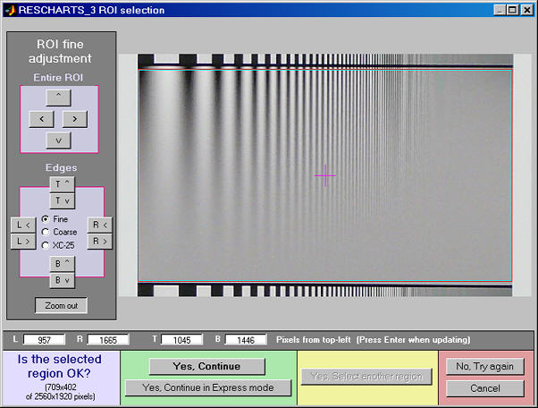
Crop for the Log Frequency-contrast chart. Leave a small margin
(1/2 - 1% of the image height) at the top and bottom.
If Express mode is not selected, the input dialog box shown on the right appears. Since this dialog box is used for several modules, some entries, such as Color space and SQF, are not relevant to Log F-Contrast.
Gamma is used to linearize the test chart. It can be measured by Stepchart, Colorcheck, or Multicharts. 0.5 is a typical value for color spaces intended for display at gamma = 2 2 (sRGB, Adobe RGB, etc.).
Channel is R, G, B, or Y (luminance; the default).
MTF plots selects the x-axis scaling. If Cycles/inch or Cycles/mm are selected, the pixel spacing (um/pixel, pixels/inch, or pixels/mm) should be entered.
X-axis scaling for linear plots selects the maximum spatial frequency to be displayed. |
|
Don't worry about getting all settings correct: You can always open this dialog box by clicking on Image settings & options in the Rescharts window.
After you press OK, calculations are performed and the most recently-selected display appears.
Output
The Display box in the Rescharts window, shown below, allows you to select any of several displays. Display options are set in boxes that appear below Display. All displays except Exif data have a channel selection option (Red, Green, Blue, or Luminance (Y) (0.3R + 0.59G + 0.11B).
| Display |
Description |
| Pattern (original and linearized) |
Show pattern: normalized pixel levels (max contrast) on top; linearized (max contrast and selected row) on bottom |
| MTF (Linear frequency scale) |
Display MTF for several contrast levels (rows 1-22 in steps of 3, where the chart is divided into 25 rows for analysis) with a linear frequency scale. |
| MTF (log frequency scale) |
Display MTF for several contrast levels (rows 1-22 in steps of 3) with a log frequency scale. A thumbnail of the pattern is also displayed on the same scale. |
| MTF/contrast (2D pseudocolor contour) |
Only affects the bar region; not important for this pattern. |
| MTFnn (frequency where MTF = nn%) |
Displays MTFnn or MTFnnP (frequencies where MTF = nn% of low frequency values or peak, respectively). Displayed in selected frequency units (cycles/pixel, LW/PH, etc.) or normalized |
| EXIF data |
Show EXIF data if available. |
In addition to the displays, two buttons allow you to save results. |
| Save screen |
Saves an image of the Starchart window as a PNG file. If you check Display screen in the Save screen dialog box, the image will be opened in the editor/viewer of your choice. (Irfanview works well, and it's free.) |
| Save data |
Saves detailed results in a CSV file that can be opened by Excel and also in an XML file. |
Pattern (original and linearized)
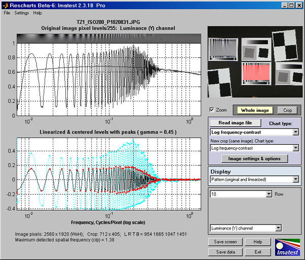
Pattern: original and linearized
The entire Rescharts window is shown. The upper plot is the normalized pixel level (pixel level/255 for bit depth of 8) of the top of the image (row 1 of 25; where contrast is maximum). The lower (linearized) plot allows the row to be selected: The cyan plot is the top of the chart (the highest contrast). Note that row 10, which is displayed in black, has much less sharpening (much less of a peak around 0.2 cycles/pixel) than maximum contrast row 1.
MTF
The display on the right shows unnormalized MTF on a linear frequency scale for several contrast bands (rows) of the chart, which is divided into 25 rows for analysis, with the highest contrast at the top and lowest at the bottom. MTF is displayed for rows 1, 4, 7, 10, 13, 16, 19, and 22.
The dark lines have been strongly smoothed. The pale dashed lines are the unsmoothed results: the fine detail consists of calculation artifacts caused by phase variations and noise; it has no significance.
An unnormalized or normalized plot may be selected in a dropdown menu in the plot settings area.
The maximum display frequency, the display scale (cycles/pixel, cycles/mm, cycles/in, or LW/PH (Line Widths per Picture Height, where 2 Line Widths = 1 cycle or line pair)), and gamma can be set to any of several options by pressing the Image settings & options button.
The printed results beneath the plot shows the contrast (at low spatial frequencies) and MTFnn and MTFnnP (the spatial frequencies where response falls to nn% of the low frequency and peak values, respectively) for nn = 50, 20, and 10%, and for rows 1, 4, 7, 10, 13, 16, and 19. The same results appear beneath the 2D pseudocolor and MTFnn displays. |
MTF: Panasonic TZ1, ISO 200,
Linear frequency scale
|
The display on the right shows the same MTF results, normalized and plotted on a logarithmic frequency scale. Normalization makes it easier to compare MTF falloff and to visually determine MTFnn. A vertically squeezed version of the image is shown just above the plot. Row 22 (very low contrast) is omitted because normalization exaggerates noise unacceptably. The contrast for each row is shown in the table below the image. |
MTF: Panasonic TZ1, ISO 200, Log frequency scale |
MTF/contrast (2D pseudocolor contour)
This selection produces the most detailed results. It has several options:
Parameter determines which parameter to display.
| Parameter |
Description |
|
| MTF (envelope- standard) |
Displays MTF, which decreases with chart contrast (height in the 2D pseudocolor display). The chart is divided into 25 rows for analysis.
MTF at low spatial frequencies is equal to chart contrast. |
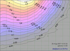 |
| Normalized contrast level |
Displays MTF normalized to 1 at low spatial frequencies for all chart contrast levels.
This may be the most generally useful display because it clearly shows how response changes with contrast level (with the low spatial frequency contrast level removed).
In a camera with uniform signal processing (i.e., the same sharpening and noise reduction throughout the image, regardless of the presence of edges), the contour lines would be vertical. Most cameras have a degree of sharpening (high frequency boost) in the presence of contrasty edges and noise reduction (high frequency attenuation) in their absence. This is evident in the display on the right (explained in more detail below). |
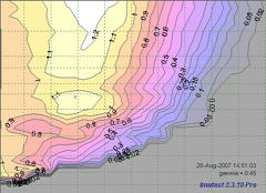 |
| Normalized contrast loss |
Displays MTF
normalized to 1
- at low spatial frequencies for all chart contrast levels, and
- at the maximum contrast level for all spatial frequencies (the top of the chart).
Results can be difficult to interpret, especially in the presence of noise. |
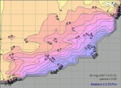 |
Style selects the frequency scale and whether to show a color bar to the right of the main display.
| Style |
Description |
| Log frequency |
The horizontal axis displays frequency on a logarithmic scale. The maximum display frequency can be set by pressing Image settings & options. |
| Log frequency, color bar |
The horizontal axis displays frequency on a logarithmic scale. The maximum display frequency can be set by pressing Image settings & options. A color bar showing the color scale is displayed to the right of the main plot. |
| Linear frequency |
The horizontal axis displays frequency on a linear scale. |
| Linear frequency, color bar |
The horizontal axis displays frequency on a linear scale. A color bar showing the color scale is displayed to the right of the main plot. |
The displays on the right show the Normalized contrast level (MTF normalized to 1 at low spatial frequencies for all chart contrasts) for the Panasonic TZ1 camera with ISO speed set at 80 (right) and 800 (right, below). Spatial frequency is displayed on a linear scale with a maximum frequency of 0.5 cycles/pixel (selectable by pressing Image settings & options ).
The image on the right (ISO 80) shows significant sharpening at moderate to high contrasts: peak normalized contrast is 1.2 or more for chart contrast greater than 0.4 and 1.1 or greater for chart contrast greater than 0.11. The amount of sharpening decreases gradually with chart contrast, ad evidence by the moderately slanted contour lines between 0.9 and 0.1 at contrasts over 0.1. |
Normalized contrast: Panasonic TZ1, ISO 80
|
The difference between the two images is striking. At ISO 800 the TZ1 has much less sharpening and more noise reduction— and correspondingly less detail. The amount of sharpening decreases more rapidly with contrast than for the ISO 80 case, as shown by the much more slanted contour lines.
|
Normalized contrast: Panasonic TZ1, ISO 800 |
MTFnn (frequencies where MTF = nn% of low frequency or peak values)
This selection produces a concise summary of results for this module. It has several options:
| Parameter |
Description |
| MTFnn |
The spatial frequency where MTF drops to nn% of its low frequency value. Curves are plotted for nn = 70, 50, 30, 20, and 10 (%). MTF50 is the most frequently used result; it corresponds to bandwidth in electrical engineering. The horizontal axis is the original chart contrast (analyzed in 24 rows). The vertical axis is the MTF frequency. Its scale (cycles/pixel, cycles/mm, cycles/in, or LW/PH) can be set by pressing Image settings & options. |
| MTFnnP |
The spatial frequency where MTF drops to nn% of its maximum (peak) value. Identical to MTFnn for unsharpened or moderately sharpened images, but it can be lower for strongly sharpened images, which have a distinct response peak. It has a slightly better correlation to perceived sharpness than MTFnn. Horizontal and vertical axes are identical to MTFnn. |
| MTFnn NORMALIZED |
The spatial frequency where MTF drops to nn% of its low frequency value, normalized to 1 at low spatial frequencies. This allows the percentage change of MTFnn with chart contrast (horizontal axis) to be conveniently compared. |
| MTFnnP NORMALIZED |
The spatial frequency where MTF drops to nn% of its maximum (peak) value, normalized to 1 at low spatial frequencies. This allows the percentage change of MTFnn with chart contrast (horizontal axis) to be conveniently compared. |
The plots on the right show MTF70 through MTF10 in units of Cycles/Pixel for the Panasonic TZ1 camera with ISO speed set at 80 (right) and 800 (right, below). They are derived from the same images as the Normalized contrast level plots, above.
The MTFnn units (Cycles/pixel to Cycles/mm, Cycles/in, or LW/PH) can be selected using the Image settings & options button. |
MTF70-MTF10: Panasonic TZ1, ISO 80
|
At ISO 800 the TZ1 has much lower MTFnn for all values of nn from 70 through 10. Note that the vertical scales are different: 0.5 (above; ISO 80) vs. 0.35 (right; ISO 800).It also falls off much more rapidly with contrast; evidence of stronger noise reduction, i.e., nonlinear signal processing.
The MTFnn display shows the changes in performance between different settings (ISO 80 and 800 in this case) more clearly than the 2D pseudocolor contour plots, above, even though (or perhaps because) it contains less detail. |
MTF70-MTF10: Panasonic TZ1, ISO 800 |
Star Chart
Analysis of the Siemens star chart
| New in Imatest 2.7.2 The number of calculation radii to be selected (32 (fastest), 64, or 128). It was formerly always 32; the default is now 64. There is an additional option for low frequency MTF normalization. Calculations have been optmized for consistency and speed. Bumps ( "Scallop" patterns) previously noted in MTF response have been tamed. |
Introduction
Star Chart, which uses the Rescharts interface, measures SFR (Spatial Frequency Response) or MTF (Modulation Transfer Function) from the sinusoidally-modulated Siemens star chart proposed for inclusion in a future release of the ISO 12233 standard, as described in A Pilot Study of Digital Camera Resolution Metrology Protocols
Proposed Under ISO 12233, Edition 2. The Siemens star chart has been strongly promoted by Image Engineering, a supplier of test charts and hardware located near Köln, Germany. Their paper, Digital Camera Resolution Measurement Using Sinusoidal Siemens Stars, is a valuable reference (as are their other technical publications).
Charts with 144, 72, and 48 cycles can be analyzed in 8, 12, or 24 segments around the circle. The value of gamma used to linearize the chart can optionally be determined from the 16 small square patches near the edge of the chart or it can be measured externally and entered.
Creating and photographing the chart and running the program
Star Chart measures MTF using calculations similar to Log Frequency. The principal difference is that is measures it for a range of angles (in 8, 12, or 24 segments) using a sinusoidally-modulated pattern along the radii of a circle. This method is more direct than the slanted-edge method, but may be slightly less accurate. Because calculations are performed on circles of known spatial frequencies, the calculation can be made more robust against noise than Log Frequency.
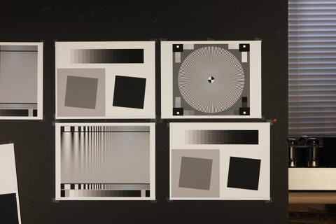
Image with star chart (upper right)
The image above used to illustrate the Star chart module and to compare results with Slanted-edge SFR and Log Frequency. It was captured with a Canon EOS-40D camera, 24-70mm f/2.8L lens set at 50mm, f/5.6, ISO 100. It includes Star, Log Frequency-Contrast and slanted-edge charts with high and low contrast (20:1 and 2:1).
Purchase test charts from Image Engineering or create them using Imatest Test Charts, then print the chart on a high quality inkjet printer. Recommended Test Charts options are PPI: 720 (Epson inkjets) or 600 (HP or Canon inkjets), Height (cm) (as required), Highlight color: White, Contrast ratio: 40, Type: Sine, Gamma: 2.2, Star pattern bands: 144 or 72, Chart lightness: Lightest, ISO standard chart: Yes or Yes (small inner circle) (inner circle has 1/10 or 1/20 the diameter of the outer, respectively).
| Number of chart cycles Ideally the maximum spatial frequency (just outside the inner circle) should be around 0.6 to 1.0 cycles/pixel. The diameter of the inner circle di is 1/10 or 1/20 times the diameter dP of the circular sine pattern, depending on the chart (selectable in Test Charts). The smallest diameter for analysis is 0.11dP or 0.056dP. For an image of P pixels (width or height) of a star with N cycles, where the pattern circle diameter dP takes up a fraction g of P (dP = gP; di = 0.11 gP ( or 0.056 gP ) ) , the maximum spatial frequency in cycles/pixel is
fmax = N / (0.11 π dP) = N / (0.11 π g P) (inner circle 1/10 the diameter of the outer)
fmax = N / (0.056 π dP) = N / (0.056 π g P) (inner circle 1/20 the diameter of the outer)
Example: for a 3000 pixel wide image where the pattern circle dP takes up g = 0.25 (25%) of the image and the inner circle has 1/10 the diameter, fmax = 0.555 cycles/pixel for a 144-cycle pattern; fmax = 0.278 cycles/pixel for a 72-cycle pattern. The 144-cycle pattern is indicated. 72-cycle patterns are most suitable for low resolution cameras (~2 megapixels or less). |
Mount the chart on a flat dark board— 1/2 inch foam board works well; thinner board warps more easily. Depending on the number of horizontal pixels in the chart to be analyzed, the chart should occupy 1/3 to 1/4 of the horizontal frame. Other charts can be mounted along with it.
Orientation. The pattern should be oriented horizontally, i.e., in landscape orientation (it is slightly wider than high).
Photograph the chart using the sort of lighting described in Imatest Lab or How to test lenses, taking care to avoid glare. Save the image in any one of several high quality formats, but beware of JPEGs with high compression (low quality), which will show degraded quality, unless, of course, you are testing JPEG degradations.
Because resolution varies over the image for most cameras and lenses, the star chart should not take up too much of the frame— in most cases its diameter should be no more than 1/3 of the image height.
Open Imatest, then click on Rescharts. The Rescharts window is described in the Rescharts page.
Select a pattern to analyze (in this case, Star Chart ) by clicking on one of the entries in the popup menu below Chart type or by clicking on Read image file if Star Chart is displayed. The Read image file button and popup menu (shown on the right) are highlighted (yellow background) when Rescharts starts. |
|
Select the image to read. If the pixel size is the same as the previous Star Chart run, you'll be asked if you want to use the previous ROI, adjust the previous ROI, or crop anew. If the folder contains meaningless camera-generated file names such as IMG_3734.jpg, IMG_3735.jpg, etc., you can change them to meaningful names that include focal length, aperture, etc., with the View/Rename Files utility, which takes advantage of EXIF data stored in each file.
Cropping The initial crop should include the entire pattern, including the outside of the black rectangles (with the small white squares inside). It doesn't have to be precise because it will be refined in the ROI fine adjustment window, shown below. The ROI fine adjustment window may be maximized to facilitate fine selection.
In the ROI fine adjustment window the pattern should be cropped so
- the middle cyan square is at the bounds of the large star pattern circle (or slightly inside if there is distortion),
- the inner cyan square is on the inner circle (which consists of four quadrants— two white, two black) for inner circles with 1/10 the diameter of the outer. (The inner circle will be well inside of the inner cyan square for small inner circles, which have 1/20 the diameter.),
- the magenta crosshair inside the inner circle is well-centered. If it is slightly off Imatest will automatically correct it.
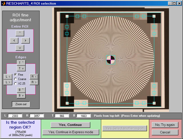
ROI fine adjustment window showing the cropped Star Chart image
Canon EOS-40D camera, 24-70mm f/2.8L lens
set at 50mm,
f/5.6, ISO 100.
Click on image to load full-size test image.
If Express mode is not selected, the input dialog box shown below appears. Some buttons such as SQF Options are inactive: they are holdovers from other modules reserved for future use. This dialog box can be at any time by pressing the Image settings & options button.
Settings
Calc segments is the number of segments around the circle to display in the analysis. 8, 12, and 24 are supported. 8 is the default.
Calc. radii is the number of radii on the circle used for the MTF calculations. It was 32 prior to version 2.7.2. 64 is considerably more accurate but slightly slower (it's the new default). 128 is slightly more accurate and slower still.
Normalization selects the MTF normalization method (where to set MTF to 1.0):
- normalize to the outer MTF value for each segment (the default),
- normalize to the maximum outer MTF value in all segments, or
- normalize to the difference between the lightest and darkest of the square patches near the pattern edge.
(1) may be slightly better when illumination is nonuniform. (2) may be slightly better when actual MTF varies between segments. (3) is simetimes better because the lowest spatial frequencies in the star may not be low enough approximate zero spatial frequency.
Channel is R, G, B, or Y (luminance; the default).
|
Image settings & options dialog box |
Inner circle May have either 1/10 or 1/20 the diameter of the outer. Should match the chart. Affects the maximum spatial frequency of the analysis.
Enter or calculate gamma Choose between Calculate gamma & linearize from chart patches or Enter gamma for linearization. If Calculate gamma... is selected, the 16 small square patches at the periphery of the star chart are used to determine the value of gamma for linearizing the chart, Gamma (below) is disabled, and the displayed value of gamma includes the indicator (chart).
Gamma is used to linearize the test chart when Enter gamma... (above) is selected. It can be measured by Stepchart, Colorcheck, or Multicharts. 0.5 is a typical value for color spaces intended for display at gamma = 2 2 (sRGB, Adobe RGB, etc.). If gamma is entered (rather than calculated), the displayed value of gamma includes the indicator (input).
Display options
MTF plots selects the x-axis scaling. If Cycles/inch or Cycles/mm are selected, the pixel spacing (um/pixel, pixels/inch, or pixels/mm) should be entered.
X-axis scaling for linear plots selects the maximum spatial frequency to be displayed in linear plots.
Don't worry about getting all settings correct: You can always open this dialog box by clicking on Image settings & options in the Rescharts window.
After you press OK, calculations are performed and the most recently-selected display appears.
Output
The Display box in the Rescharts window, shown below, allows you to select any of several displays. Display options are set in boxes that appear below Display. All displays except Exif data have a channel selection option (Red, Green, Blue, or Luminance (Y) (0.3R + 0.59G + 0.11B).
| Display |
Description |
| MTF (original and linearized) |
MTF for up to 8 segments of the star. Both linear and logarithmic frequency displays are available. |
| MTFnn or MTFnnP |
Display MTFnn (the frequencies where MTF equals nn % of the low frequency values) and MTFnnP (the frequencies where MTF equals nn % of the peak value) for nn = 70, 50, 30, 20, and 10. Both polar (spider) and rectangular plots are available. |
| MTF contours (rectangular) |
Display MTF contours in a rectangular plot with linear or logarithmic frequency display. Similar to the MTFnn rectangular plot. |
| MTF contours (polar) |
Display MTF contours in a polar plot whose geometry duplicates that of the target. |
| EXIF data |
Show EXIF data if available as well as linearization curves (used to calculate gamma from the chart). |
In addition to the displays, two buttons allow you to save results. |
| Save screen |
Saves an image of the Starchart window as a PNG file. If you check Display screen in the Save screen dialog box, the image will be opened in the editor/viewer of your choice. (Irfanview works well, and it's free.) |
| Save data |
Saves detailed results in a CSV file that can be opened by Excel and also in an XML file. |
The spatial frequency is automatically calculated from the image, under the assumption that log frequency increases linearly with distance. The number of chart cycles is also determined automatically.
MTF
The MTF (Spatial Frequency Response) can be displayed on a linear or logarithmic frequency scale. You can select between showing the first 8 segments equally weighted, or emphasizing any of the segments (Segment 1 is shown as a thick black line below). The average response is a thick magenta-gray line. Smoothed, interpolated response is normally displayed, but uninterpolated, unsmoothed (raw) response is available as an option.
Normalization: MTF is normalized (set to 1.0) using either (1) MTF at the outer radius of each segment, (2) the maximum value of MTF at the outer radii of all segments, or (3) the difference between the lightest and darkest square near the pattern edge. Neigher case (1) nor (2) is ideal because the minimum spatial frequency is not as low as it should be for correct normalization. (The high to low spatial frequency ratio is only 10 or 20 for the star chart — much lower than for the Log Frequency or Log F-Contrast charts.) In general, normalizing MTF to the outer radius of the star increases MTF slightly above its true value. MTF should ideally be normalized to a lower spatial frequency. Case (3) should only be used with maximum contrast patterns.
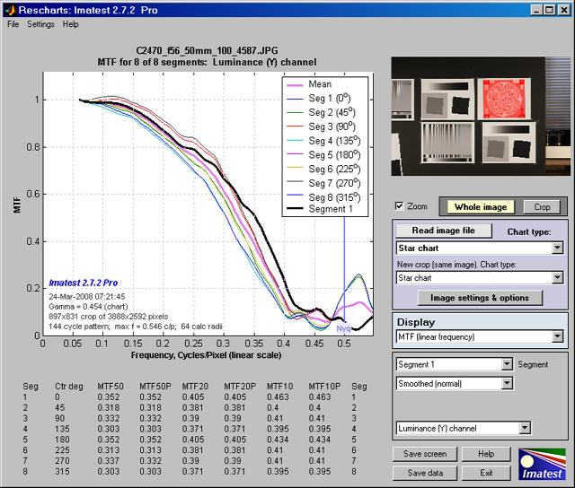
MTF (linear frequency scale) for 8 segments of the Star pattern
The entire Rescharts window is shown. The original 64 radii are linearly interpolated to 101 frequencies, then smoothed to eliminate response roughness caused by calculation artifacts and noise. Gamma = 0.454 (chart) at the lower left of the plot indicates that gamma was calculated from the 16 small square patches at the periphery of the chart. If it were calculated elsewhere and entered into Star Charts, (input) would be displayed instead of (chart).
MTF50, MTF50P, MTF20, MTF20P, MTF10, and MTF10P for the first 8 segments are displayed in a table below the plot for this and several of the output plots (but not shown below).
MTFnn, MTFnnP
The plot on the right shows MTF70 through MTF10 (spatial frequencies where MTF = 70,, 50, 30, 20, and 10%) on a linear frequency scale displayed in rectangular (Cartesian) coordinates. Frequency is displayed in cycles/pixel, but Line Widths per Picture Height (LW/PH), cycles/inch, or cycles/mm can be selected by pressing the Image settings & options button. The full circle is shown: segment 9 corresponds to segment 1: (0 degrees center angle).
The legend (the box on the right) has been moved using the mouse to uncover the MTF10 (blue) line.
|
MTF70 – MTF10: Rectangular (Cartesian)
coordinates,
Linear frequency scale.
|
The plot on the right shows MTF70 through MTF10 displayed in polar coordinates. Spatial frequency (cycles per pixel in this case) increases with radius. (This is the opposite of the image itself, where spatial frequency is inversely proportional to radius.)
This plot is most similar to the spider plot shown in Image Engineering digital camera tests and Digital Camera Resolution Measurement Using Sinusoidal Siemens Stars (Fig. 15), by C. Loebich, D. Wueller, B. Klingen, and A. Jaeger, IS&T, SPIE Electronic Imaging Conference 2007. MTF10 (the black octagon on the right) corresponds to the Rayleigh diffraction limit. |
MTF70 – MTF10: Polar coordinates,
Linear frequency on radius.
|
MTF contours: rectangular and polar
The plot on the right shows the MTF contours for each of the 8 segments. Spatial frequency is displayed on a linear scale, but a log scale may be selected and a color bar (see below) may be added.
This plot contains information similar to the rectangular MTFnn plot, above. |
MTF contours, rectangular display,
Linear frequency scale.
|
The plot on the right shows the MTF contours for each of the 8 segments, displayed on a polar scale, where location (radius) on the plot corresponds to the image. This is the inverse of the polar MTFnn plot, above, where spatial frequency is the inverse of image radius.
Most of the action in this image is near the center. If the Zoom box is checked you can zoom in by selecting a portion of the image or simply by clicking on it. |
MTF contours, polar display. |
Equations, algorithm, and issues
Equations for analyzing the Siemens star are given in Digital Camera Resolution Measurement Using Sinusoidal Siemens Stars by C. Loebich, D. Wueller, B. Klingen, and A. Jaeger, IS&T, SPIE Electronic Imaging Conference 2007. The algorithms used for Imatest Star Charts are similar, differing only in details. The 32, 64, or 128 radii ri , located from just outside the inner circle to just inside the outer circle, are selected using a logarithmic scale that makes them more closely spaced near the inner circle. This makes the frequency spacing (proportional to 1/radius) more consistent than for uniformly spaced radii. For each of the 32 radii ri , all points are located with radii between ( ri-1+ri )/2 and ( ri+ri+1 )/2 pixels. ( ri−0.7 and ri+0.7 pixels, used prior to Imatest 2.7.2, caused significant bumps in the MTF response.) Spatial frequency is 1/(2π ri ) cycles/pixel. These points fit the curve,
I(φ) = a + b1 sin(2π/g) φ ) + b2 cos(2π/g) φ ), where b = sqrt( b12 + b22 )
MTF = b/a
The equation for I(φ) is recognized as a term in a Fourier series expansion, which can be solved using the standard Fourier series equation since each segment (there are 8, 12, or 24) has an integral number of cycles (of a total of 144, 120, 72, or 48 cycles on the chart).
b1 = k mean( sin(2π/g) I(φ) ); b2 = k mean( cos(2π/g) I(φ) ); a = mean( I(φ) )
Since MTF is normalized to 1 at the lowest measured spatial frequency for each segment, k drops out of the final result.
Algorithm issues
Bumps in the MTF response curve caused by aliasing are visible in the image below.
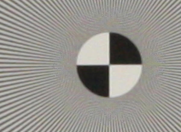
3x enlarged image of the center of a star pattern acquired on the Canon EOS-40D,
24-70mm f/2.8 lens set to 50mm, f/8 (a sharp setting)
Normalization: MTF is normalized using (1) MTF at the outer radius of each segment, (2) the maximum value of MTF at the outer radii of all segments, or (3) the difference between the lightest and darkest square near the pattern edge. Neither case (1) nor (2) is ideal because the minimum spatial frequency is not as low as it should be for correct normalization. (The high to low spatial frequency ratio is only 10 or 20 for the star charts — much lower than for the Log Frequency or Log F-Contrast charts.) In general, normalizing MTF to the outer radius of the star increases MTF above its true value. MTF should ideally be normalized to a lower spatial frequency, as with case (3), which should only be used with maximum contrast charts. |
Using Uniformity (Light Falloff)
Measures light falloff (lens vignetting) and sensor nonuniformity
Light Falloff (Uniformity) measures lens vignetting (dropoff in illumination at the edges of the image) and other image, illumination, and sensor nonuniformities. For example, it can measure evenness of flash illumination (using light bounced off a white wall) or the uniformity of flatbed scanners. In Imatest Master, Light Falloff can also display a pixel level histogram, analyses of hot and dead pixels and color shading, and a detailed image of fine nonuniformities (i.e., sensor noise). These features are described in Light Falloff instructions: Imatest Master .
New in Imatest 3.1
Several images can be combined (averaged) to facilitate fixed pattern noise display. The hot/dead pixel display can be set to count pixels that meet the criteria for all channels, any channel (the former default), or the selected channel. The Color shading display includes several additional ΔE measurements, including ΔE 2000.
New in Imatest 2.6.7
Spot detection has been added to the fine detail display. |
Instructions
To prepare an image for Light Falloff,
- Set your camera or lens to manual focus and focus it at infinity (the worst case for light falloff).
- Photograph an evenly illuminated uniform subject.
- One of the simplest ways to obtain a uniform subject is to photograph your computer monitor at a distance of 1-3 inches (2-8 cm) using the Imatest Screen Patterns module, shown on the right. Click on Screen Patterns on the right of the Imatest main window, then maximize the screen. You can adjust the Hue, Saturation, and Lightness (H, S, and L, which default to 0,0,1) if required. (Thanks to Jonathan Sachs for this suggestion.)
This method works best with flat screen LCDs with wide viewing angles.
- For extreme wide angle lenses or laptop screens with a limited viewing angle, an additional diffuser should be used. We recommend using opal diffusing glass mounted close to the lens. Opal glass is available in the US from Edmund Optics. (Thanks to Bart van der Wolf for the suggestion.) If a diffuser is used, a lightbox may be substituted for the monitor. (Lightboxes are typically brighter but less uniform.)
|
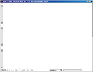
Screen Pattern module for Light Falloff. |
- This technique is less effective with CRTs. L may need to be reduced to keep exposure time longer than 0.1 seconds so the raster scan doesn't cause uneven exposure. The Canon EOS-40D exposure metering seemed to fail as a result of the raster scan.
- (We prefer the monitor, but this approach may be useful in come cases.) Photograph an evenly-lit smooth sheet of matte paper (white or gray). Get close to the subject, but not so close that you shade it. Outdoors illumination (shade) sometimes results in the most even illumination. Getting uniform illumination can be a challenge with ultrawide lenses, such as the Canon10-22 mm digital zoom lens set to 10mm (equivalent to 16 mm in the 35mm format); it's almost impossible to avoid shading part of the card. The computer monitor (above) is strongly preferred in such cases.
|
- The subject does not need to be in focus (you don't even need a lens to measure sensor uniformity); the goal is to measure lens light falloff and/or sensor uniformity, not features of the subject.
- For typical lens vignetting measurements, set exposure compensation to overexpose by about one f-stop. (You may, however, use any exposure you choose.)
- Save the image as a RAW file or maximum quality JPEG.
To obtain truly even illumination
for precision scientific measurements you'll need an integrating sphere from a supplier such as SphereOptics, Labsphere, or Electro-Optical Industries (EOI). The SphereOptics system on the right is about $8,000, including variable attenuator, power supplies, operating software, and calibration. It is available in sizes from 4 to 76 inches.
The Labsphere USS-1200 or USS-1200V and the EOI ISV 400, all 12 inches in diameter with 4 inch exit ports, are ideal for SLRs. Smaller models will work with compact digital cameras.
Integrating spheres aren't cheap. Less expensive alternatives include Kyoritsu calibrated light sources (especially the pattern light boxes), available in the North America from C.R.I.S. Tsubosaka (Japan) also has some interesting products. There are no obvious US or European distributors. |
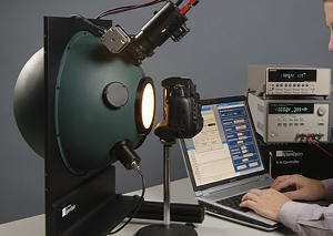 |
To run Light Falloff,
- Start Imatest and click on Light Falloff.
- Very large files (height x width x colors over 40 MB) may cause memory overflow problems. Files over 40 or 80 MB can be automatically reduced 1/2x linearly (using 1/4 the memory). Click Settings, Options and Settings I... (in the Imatest main window) and make the appropriate setting in LARGE FILES (Light Falloff, Distortion).
- Open the image file.
| Multiple file selection Several files can be selected in Imatest Master using standard Windows techniques (shift-click or control-click). Depending on your response to the multi-image dialog box you can combine (average) several files or run them sequentially (batch mode). |
Combined (averaged) files are useful for measuring fixed-pattern noise (at least 8 identical images captured at low ISO speed are recommended). The combined file can be saved. Its name will be the same as the first selected file with _comb_n appended, where n is the number of files combined. |
Batch mode allows several files to be analyzed in sequence. There are three requirements. The files should (1) be in the same folder, (2) have the same pixel size, and (3) be framed identically. |
The input dialog box for the first run is the same as for standard non-batch runs. Additional runs use the same settings. Since no user input is required they can run extremely fast. |
If the order of the files in a batch runs is different from the selection order, click Settings, Options and Settings... (in the Imatest main window) and change the setting in Batch run order. The sequence may be affected by Windows Explorer settings. |
One caution: Imatest can slow dramatically on most computers when more than about twenty figures are open. For this reason we recommend checking the Close figures after save checkbox, and saving the results. This allows a large number of image files to be run in batch mode without danger of bogging down the computer. |
|
- Three cropping (ROI selection) options are available by clicking Settings, Options and Settings... in the Imatest main window. These include
| Don't ask to crop. (Use settings in LF input dialog box.) |
| Select crop by dragging cursor. Ask to repeat crop for same sized image. |
| Select crop by dragging cursor. Do not ask to repeat crop. |
Although the first option (Don't ask to crop...) was the default prior to Imatest 2.3.12, the second option (Select crop by dragging cursor. Ask to repeat crop for same sized image), which is similar to the ROI selection in SFR, may be preferred.
- A dialog box appears. The following settings appear in all Imatest versions. Imatest Master settings are shown below.
- Title Defaults to the file name. You can change it if you wish.
- Display Light Falloff contour plots (Plot area; on by default).
Turns the main light falloff contour plots off or on. Normally on (checked), but may be turned off by Imatest Master users interested in other results, such as hot/dead pixels and color shading. Four display options are available. Normalized refers to the first (level) plot only.
Contours superposed on image
(not normalized) |
Contours superposed on image
(normalized to 1) |
Pseudocolor with colorbar
(not normalized) |
Pseudocolor with colorbar
(normalized to 1) |
|
 Input dialog box in Imatest Studio
 |
- Gamma (Settings area). The default value of gamma, 0.5, is typical for digital cameras. Gamma affects the second figure (the light falloff measured in f-stops); it has no effect on the first figure. Gamma can be measured by Stepchart using any one of several widely-available step charts. (Reflection charts are easiest to use but transmission charts can also be used to measure dynamic range.) Some issues in calculating gamma are discussed below the second figure.
- Corner and side regions (default 32x32 pixels) allows you to select the areas at the corners and sides of the images to be analyzed. Choices include 10x10 pixels, 32x32 pixels, 1% (min. 10x10), 2% (min. 10x10), 5%, and 10%.
- Crop pixels near borders (L, R, T, B) (Settings area). If checked, the image is cropped by the number of pixels indicated near the left, right, top, and bottom borders.
The following options are available in Imatest Master only. They are discussed in detail in Light Falloff instructions: Imatest Master .
- Channel (Settings area) You can choose between Red, Blue, Green, and Y (luminance) channel
- Hot and dead pixels (Settings area) By checking the appropriate boxes you can display hot pixels (red x) and/or dead pixels (blue •). Hot pixels are stuck at or near the sensor's maximum value (255 in 8-bit files) and dead pixels are stuck at or near 0.
Because signal processing— especially JPEG compression— can cause these values to shift, you can use the sliders to set the detection threshold between 6-255 for hot pixels and 0-249 pixels for dead pixels. (The extreme values are for measurements made on white or black fields.) Clicking on < or > at the ends of the sliders adjusts the threshold by 1. The default values are 252 and 4, respectively. Settings are saved between runs. JPEG files must be saved at the highest quality level for this feature to work; isolated hot and dead pixels tend to be smudged at lower quality levels. Details are described in Light Falloff: Imatest Master .
|
Input dialog box in Imatest Master |
- (Plot area) Color shading displays color nonuniformity. Several options are available. Display Histogram displays histograms of R, G, and B channels. Display color uniformity profiles displays R, G, and B values (or ratios— several options available) along the diagonals and horizontal and vertical center lines. Display fine detail displays a detailed figure of noise and sensor uniformity. The calculation can be slow and uses lots of memory. Details in Light Falloff: Imatest Master .
Results
The first figure: luminance contour plot
shows normalized pixel level contours for the image file luminance channel, where luminance is defined as Y = 0.30*R + 0.59*G + 0.11*B.. A maximum value of 1 corresponds to pixel level = 255 for image files with a bit depth of 8 or 65535 for a bit depth of 16. Some illumination nonuniformity is evident in the plot: the top is brighter than the bottom. The image is smoothed (lowpass filtered) before the contours are plotted.
The text displays the maximum normalized pixel level for the luminance channel, the worst and mean corner values (in normalized pixel levels and as a percentage of maximum), and the side values. Selected EXIF data is shown on the right. Two hot and two dead pixels (which were simulated) were detected with thresholds of 246 and 10 (pixels), respectively. The crop (Left, Right, Top, Bottom) is shown just below. Details below.
The setting for correcting light falloff in the Picture Window Pro Light falloff transformation is also given. The PW pro Light Falloff dialog box is shown on the right. Film Size (mm) remains at 36 (the PW Pro default value: the width of a 35mm frame). Picture Window Pro is the powerful and affordable photographic image editor that I use for my own work. The Lens Focal Length is rarely the exact focal length of the lens. Light falloff depends on the lens aperture (f-stop) as well as a number of lens design parameters. Lenses designed designed for digital cameras, where the rays emerging from the rear of the lens remain nearly normal (perpendicular) to the sensor surface, tend to have reduced light falloff.
For aesthetic purposes I generally recommend undercorrecting the image, i.e., using a larger Lens Focal Length. This makes the edges somewhat darker, which is usually pleasing. Ansel Adams routinely burned (darkened) the edges of his prints. Part of the reason was that he had to compensate for light falloff from his enlarger (when he wasn't contact printing).
"My experience indicates that practically every print requires some burning of the edges, especially prints that are to be mounted on a white card, as the flare from the card tends to weaken visually the tonality of the adjacent areas. Edge burning must never be overdone..."
Ansel Adams, "The Print," p. 66. 1966 edition.
The second figure: f-stop contour plot
shows image file luminance contours, measured in f-stops, normalized to a maximum value of 0. A pseudocolor display with color bar has been selected. The colors in the color bar are fixed: colors always vary from white at 0 f-stops to black at -4 f-stops and darker. For this plot to be accurate, a correct estimate of gamma (the camera's intrinsic contrast) is required. Gamma is measured by Stepchart, using any one of several widely-available step charts, or by Colorcheck.
Gamma can be tricky to measure for several reasons. (1) Many cameras have complex response curves, for example, "S"-curves superposed atop gamma curves. This means that gamma can vary with brightness. (2) Some cameras employ adaptive signal processing in their RAW conversion algorithms. This increases contrast (i.e., gamma) for low contrast subjects and decreases it for contrasty subjects. This improves image quality for a wide range of scenes, but makes measurements difficult, especially since Light Falloff targets have the lowest possible contrast.
Deriving f-stop falloff
The f-stop falloff in the second plot is derived from the equations,
Pixel level =
k1 luminance
γ ; Luminance =
k2 pixel level
1/γ and
F-stop loss = log
2(luminance ratio)
= 3.322 log
10(luminance ratio)
where luminance ratio is the ratio of the maximum luminance to the luminance in the area of interest, for example, the mean value of the corners.
Example: The first and second figures, above, are derived from the same image file. In the first figure, the mean pixel level at the corners relative to the center is 0.666/0.905 = 0.736 (73.6%). Since γ is assumed to be 0.5 (fairly typical of encoding gamma of digital cameras, the exposure at the corners relative to the center is 0.736
1/γ = 0 .736
2 = 0.5416. The corresponding f-stop loss = log
2(0.5416) = 3.322 log
10(0.5416) = -0.885 f-stops. There is a slight discrepancy with the second figure, which calculates the mean at the corners (0.894 f-stops)
after taking the logarithm to convert results into f-stops.
Additional figures are illustrated in Light Falloff: Imatest Master .
.CSV and XML output files
The .CSV output file contains additional statistics. Most have obvious meanings.
- Image pixels contains the width, height, and total size in pixels.
- Hot and Dead pixels show the total count and the fraction (divided to total pixels)
- The x and y coordinates of the hot and dead pixels are listed. The maximum is 100. Coordinates are in pixels from the top-left.
Contact Imatest if you need additional .CSV output.
The optional XML output file contains results similar to the .CSV file. Its contents are largely self-explanatory. It is stored in [root name].xml. XML output will be used for extensions to Imatest, such as databases, to be written by Imatest and third parties. Contact us if you have questions or suggestions.
Saving results
At the end of the run, a dialog box for saving results appears. It allows you to select figures to save and
choose
where to save them. The default is subdirectory Results in the data file directory. You can change to another existing
directory,
but new results directories must be created outside of Imatest— using
a utility such as Windows Explorer. (This is a limitation of this
version
of Matlab.) The selections are saved between runs.
You can examine the output figures before you check or uncheck
the boxes.
Figures, CSV, and XML data are saved in files whose names consist of a root file name with a suffix for plot type and channel (R, G, B, or Y) and extension. Example: IMG_9875_ISO1600_RGB_f-stop_ctrG.png. The root file name defaults to the image file name, but can be changed using the Results root file name box. Be sure to press enter.
Checking Close figures after save is recommended for preventing a buildup of figures (which slows down most systems) in batch runs. After you click on Yes or No,
the Imatest main window reappears.
|
 |
The CSV and XML files contain EXIF data, which is image file metadata that contains important camera, lens, and exposure settings. By default, Imatest uses a small program, jhead.exe, which works only with JPEG files, to read EXIF data. To read detailed EXIF data from all image file formats, we recommend downloading, installing, and selecting Phil Harvey's ExifTool, as described here.
Links
Vignetting by Paul van Walree, who has excellent descriptions of several of the lens (Seidel) aberrations and other causes of optical degradation.
Uniformity (Light Falloff): Imatest Master
Instructions for Imatest Master
This section describes Light Falloff (Uniformity) features available with Imatest Master. Light Falloff was originally intended to measure lens vignetting (dropoff in illumination at the edges of the image), but it can measure a variety of image nonuniformities— resulting from the lens, illumination, or sensor— including color shading, noise distribution, and spots from dust. Basic instructions are found in Using Light Falloff.
New in Imatest 3.1
Several images can be combined (averaged) to facilitate fixed pattern noise display. The hot/dead pixel display can be set to count pixels that meet the criteria for all channels, any channel (the former default), or the selected channel. The Color shading display includes several additional ΔE measurements, including ΔE 2000.
New in Imatest 2.6.7
Spot detection has been added to the fine detail display. |
Input dialog box
The following options are available in all Imatest versions:
- Title Defaults to the file name. You can change it if you wish.
- Display Light Falloff contour plots (Plot area; on by default).
Turns the main light falloff contour plots off or on. Normally on (checked), but may be turned off by Imatest Master users interested in other results, such as hot/dead pixels and color shading. Four display options are available. Normalized refers to the first (level) plot only.
Examples on Using Light Falloff.
| Contours superposed on image (not normalized) |
| Contours superposed on image (normalized to 1) |
| Pseudocolor with colorbar (not normalized) |
| Pseudocolor with colorbar (normalized to 1) |
- Gamma The default value of gamma, 0.5, is typical for digital cameras. Gamma affects the second figure (the light falloff measured in f-stops); it has no effect on the first figure. Gamma can be mesured by Stepchart using any one of several widely-available step charts. (Reflection charts are easiest to use but transmission charts can also be used to measure dynamic range.) Some issues in calculating gamma are discussed below the second figure.
- Corner and side regions (default 32x32 pixels) allows you to select the areas at the corners and sides of the images to be analyzed. Choices include 10x10 pixels, 32x32 pixels, 1% (min. 10x10), 2% (min. 10x10), 5%, and 10%. These regions can be used as the reference for the Color shading ΔE and ΔC calculations.
- Crop pixels near borders (L, R, T, B) (Settings area). If checked, the image is cropped by the number of pixels indicated near the left, right, top, and bottom borders. Several cropping (ROI selection) options are available by clicking Settings, Options and Settings... in the Imatest main window. These incluce
| Don't ask to crop. (Use settings in LF input dialog box.) |
| Select crop by dragging cursor. Ask to repeat crop for same sized image. |
| Select crop by dragging cursor. Do not ask to repeat crop. |
Although the first option (Don't ask to crop...) was the default prior to Imatest 2.3.12, the second option (Select crop by dragging cursor. Ask to repeat crop for same sized image), which is similar to the ROI selection in SFR, may be preferred.
Light Falloff input dialog box (for Pro).
The following options are available in Imatest Master only:
- Color shading (nonuniformity) Display the color nonuniformity, i.e., the difference between two of the three (R, G, B) channels or one of the L*a*b* color difference metrics (ΔE = sqrt(ΔL*2 + Δa*2 + Δb*2 ), ΔC = sqrt(Δa*2 + Δb*2 ), ΔE94, ΔC94, ΔE00, ΔC00 ), referred to the center of the image (either the central region, with size specified in the Corner and side regions box or the central 25% by area). Color shading often results from the angle at which light stikes the sensor. It tends to be worst in tiny pixels. Several options are available.
- Color shading Select not displayed (turns off plot), Red/Blue, Red/Green, Green/Blue, or ΔE/ΔC (various flavors & reference regions). Red/Blue (the extremes of the spectrum) is the most popular choice for displaying shading.
- Quantity to plot. On the right of the Color shading line. Select Pixels (gamma-encoded), Intensity (linear), or f-stop difference. Grayed out if ΔE/ΔC metrics are selected.
| Pixels displays the ratio of the the pixel values for the selected channels. If Normalized is checked, the plot is normalized to 1.0 (maximum). |
| Intensity (linear) removes the gamma encoding of the image file using the value of Gamma entered and displays the ratio of the intensities for the selected channels. If Normalized is checked, the plot is normalized to 1.0 (maximum). |
| F-stop displays the f-stop difference between the selected channels. If Normalized is checked, the plot is normalized to 0 (maximum). |
- Display background Select the image background: Exaggerated color or pseudo color. Exaggerated color increases the color saturation to increase the visibility of color nonuniformities. Examples are shown below.
- Normalized (Checkbox) If checked (the default), the shading plot is normalized to a maximum of 1 for pixels or intensity (linear) or 0 for f-stop difference. The unnormalized maximum and minimum values are displayed beneath the plot.
- Display color uniformity profiles Shows pixel levels along diagonal, vertical, and horizontal lines. The specific display is selected in the dropdown menu on the right. Described below.
- Display histograms Useful in diagnosing stuck (hot and dead) pixels. Described below.
- Display fine detail Display a detailed image of noise and sensor nonuniformity (examples below). Slow variations in image density— vignetting (low spatial frequencies) — are removed so that only short to medium range variations— sensor noise, dust spots, etc.— remain. The calculation can be slow and uses lots of memory because Matlab calculations are performed in double precision mathematics, which requires 24 bytes per color pixel (8 bytes per channel).
|
Several display options are available. The first displays noise exaggerated by a factor of 10. The second superposes contour plots (from a smoothed version of the image) on the noisy image. The third produces a pseudocolor image of local nonuniformities (also smoothed) with a color bar (legend) on the right. The fourth emphasises dark spots, usually caused by dust. A histogram can also be added beneath the fine detail plot.
|
|
| Exaggerated local noise (standard) |
| Local noise with added contours |
| Pseudocolor contours with colorbar |
| Spot detection w / threshold (pseudocolor) |
|
- Channel You can choose between Red, Blue, Green, or Y (luminance) channels.
- Color space Used for converting from RGB color space where L*a*b* color difference metrics are displayed.
- Hot and dead pixels By checking the appropriate boxes you can display hot pixels (red x) and/or dead pixels (blue •). Hot pixels are stuck at the sensor's maximum value (255 in 8-bit files) and dead pixels are stuck at 0. Because signal processing— especially JPEG compression— often causes these values to shift, you can use the sliders to set the detection threshold between 6-255 for hot pixels and 0-249 pixels for dead pixels. (The extreme values are for measurements made on white or black fields.) Clicking on < or > at the ends of the sliders adjusts the threshold by 1. The default values are 252 and 4, respectively. Settings are saved between runs. JPEG files must be saved at the highest quality level for this feature to work; isolated hot and dead pixels tend to be smudged at lower quality levels. Details of hot and dead pixels are presented below. You can choose whether to count a pixel as hot or dead if the criteria are met by any color channel (the default), all channels, or the selected channel.
Results
Hot and dead pixels (Imatest Master only)
Imatest Master allows you to detect hot and dead pixels. Hot pixels are stuck at or near the sensor's maximum value (255 in 8-bit files); dead pixels are stuck at or near 0. Image processing (especially demosaicing and data compression) may alter these numbers. Thresholds lower than 255 and higher than 0 are usually required, particularly for JPEG files, where isolated pixels are smeared, even for the highest quality levels. Hot and dead pixels cannot be reliably detected in JPEGs saved at lower quality levels.
The hot and dead pixels shown on the right met the criteria that they were above or below the threshold for any color channel. All channels or the selected channel could have been selected. |
2 hot, 2 dead pixels
of 8185344 total
Threshold: h= 245; d= 10
|
 |
The first figure in Light Falloff shows two simulated hot (x) and dead (•) pixels. The CSV output file on the right shows the basic statistics for the image (8185344 pixels total). h = 245 and d = 10 are the hot and dead pixel thresholds, respectively. The number and fraction of the hot and dead pixels are shown, followed by the x and y-locations of the first 100 hot and dead pixels. The Histogram plot, described below, is useful for selecting thresholds.
Color shading (nonuniformity) (Imatest Master only)
The Color shading plot displays the ratio or difference between R, G, and B channels or L*a*b* color errors (ΔE or ΔC). Two examples are illustrated below. The first shows shading as the ratio of Red to Blue (R/B) channel pixels. Plotted results have been normalized to a maximum of 1.0. Normalization makes the results relatively insensitive to white balance errors. The background shows exaggerated colors (HSV saturation S has been increased by 10x for low saturation values; less for high values.)
R/B Color shading, exaggerated color.
The second example shows the difference between the Red and Blue channels in f-stops with a pseudo color background. Plotted results have been normalized to a maximum of 0 f-stop difference.
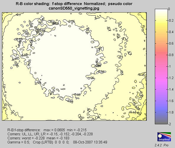
R-B (difference) color shading, pseudocolor.
Color nonuniformity can be displayed as one of the L*a*b* color difference metrics (ΔE = sqrt(ΔL*2 + Δa*2 + Δb*2 ), ΔC = sqrt(Δa*2 + Δb*2 ), ΔE94, ΔC94, ΔE00, ΔC00 ), referred to the center of the image (either the central region, with size specified in the Corner and side regions box or the central 25% by area). The ΔC metrics are of particular interest for color metrics because they omit luminance differences (ΔL*).
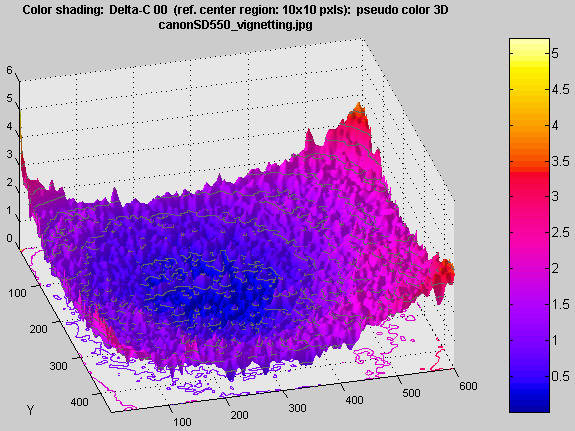
ΔC 2000 color shading (omits ΔL*), pseudocolor.
Uniformity profiles (Imatest Master only)
Uniformity profiles displays profiles of image levels along several lines: Diagonal Upper Left-Lower Right, Diagonal Lower Left-Upper Right, Vertical Top-Bottom (center), and Horizontal Left-Right (center). Several display options are listed below.
| RGBY unnormalized (max 1) |
| RGBY unnormalized pixels (max 255) |
| RGBY normalized (max 1) |
| Ratios: R/G, B/G (G constant) |
| RGBY normalized: ALL CHANNELS |
| Delta L* a* b* C* (C* = chroma) |
The independent axis goes from 0 to 1 in steps of 0.025 (41 steps total). Detailed results for the 41 steps are written to the CSV and XML output files. |
Uniformity profiles. |
Polynomial fit A fourth order fit to R, G, B, and Y (or L*, a* and b*) is shown as faint dotted lines in the upper (Diagonal UL-LR) plot. The equation for the fit is
y = c1r4 + c2r3 + c3r2 + c4r + c4
where r is the distance from the center divided ty the center-to-corner distance (r = 1 at the corners). The R, G, B, and Y coefficients are in displayed the CSV and XML output files. There is not enough space to show them in the plot. They have the following format in the CSV output file.
| Fourth order fit: y = c(1)*r^5 + C(2)*r^3 + ... + c(5) where r is normalized to center-to-corner. |
| R |
0.045 |
-0.108 |
-0.081 |
-0.083 |
0.866 |
|
|
| G |
-0.124 |
0.207 |
-0.295 |
-0.037 |
0.922 |
|
|
| B |
-0.189 |
0.315 |
-0.341 |
-0.037 |
0.907 |
|
|
Histograms (Imatest Master only)
The histogram plot, introduced in Imatest Master 2.3.11 (July 2007), facilitates the detection and the setting of thresholds for stuck (hot, dead, etc.) pixels. Histograms of log10(occurrences+1) are displayed for the red, green, and blue channels. [The logarithm compresses the plot so even a single bad pixel is visible. log10(occurrences+1) is used because log(0) = −∞ (minus infinity), while log(1) = 0.]
R, G, and B Histograms showing stuck pixels.
In this example, single stuck pixels are plainly visible near levels 0 and 252. Altough these stuck pixels were synthesized, their levels is slightly different due to JPEG compression (they were the same in a TIFF file). The dead pixel threshold is shown on the left in blue; the hot pixel threshold is shown on the right in red.
You can quickly see if the thresholds are set correctly— if they are outside the valid density region and if the dead and hot pixels are above and below their respective thresholds. You can change threshold settings and rerun Light Falloff if necessary.
Noise detail (Imatest Master only)
shows an exaggerated or pseudocolor image of the noise detail. Four options are available:
Exaggerated local noise (standard)
|
Exaggerated image of local noise |
Local noise with added contours
|
Exaggerated image of local noise with added contours |
| Pseudocolor contours with colorbar |
Pseudocolor image of local density variations. The image has been smoothed. Colors vary from image to image: the color map covers the density range of the image. |
| Spot detection w / threshold (pseudocolor) |
Pseudocolor image emphasizing spots. Fixed color map. Image is normalized to the mean density. For clarity, only densities between 0.9 and 1 are displayed in the color map. |
The local noise figures are produced by
- Subtracting a highly smoothed version of the image from the image itself. This removes broad image variations (low spatial frequencies), leaving only the fine detail. (The signal is highpass filtered.)
- Exaggerating the fine detail by a factor 5x or 10x, depending on the signal-to-noise ratio (the average pixel level of the original image divided by the standard deviation of the difference image (the results of step 1), i.e., the RMS noise).
- Adding an offset to the the exaggerated signal so the average level of the image is displayed as middle gray.
- If Local noise with added contours is selected, contours are calculated by subtracting the same highly smoothed version of the image from a moderately smoothed version of the image. Smoothing is necessarily because noise would make the contours unintelligibly rough.
The first image (below) shows noise detail for the Canon EOS-20D at ISO 1600 with the 10-22mm lens set to f/4.5. No surprises here; electronic noise dominates.
Noise detail for Canon EOS-20D, ISO 1600, 10-22mm lens, f/4.5.
The second image (below) shows noise detail for the Canon EOS-20D at ISO 100 with the 10-22mm lens set to f/8. Thanks to the small aperture, some very faint dust spots are visible. The dust is on the anti-aliasing/infrared filter/microlens assembly in front of the sensor. This assembly can be well over 1 millimeter thick. Stopping the lens down (increasing the f-stop setting) reduces the size of dust spots but makes them darker.
This image has a surprise in the form of concentric circles: bands where the noise appears to be higher or lower than the remainder of the image. This may be caused by (a) the Analog-to-Digital (A-D) converter in the image sensor chip, which can have small discontinuities when, for example going from level 127 to 128: binary 01111111 to 10000000, or (b) JPEG artifacts. Rrecall that these noniniformities are exaggerated by a factor of 10: they would be invisible or barely visible on an actual image; you might seem then faintly in smooth areas like skies.
Noise detail, Canon EOS-20D, ISO 100, 10-22mm lens, f/8.
Here is the same image, displayed in pseudocolor (which shows the amount of variation) with a color bar, and including a histogram (of individual pixels, not the smoothed image used to generate the contour plot on the left). The scale varies from image to image; it is not fixed like the scales for for the luminance and f-stop contour plots (which display long range, low spatial frequency variations). The histogram is narrower than the separate histogram image (above) because long-range (low spatial frequency) density variations have been removed. It is a good approximation to the average sensor noise.
Local nonuniformities shown in pseudocolor, Canon EOS-20D, ISO 100, 10-22mm lens, f/8.
The image below is an enlargement (a zoom) of the above image, centered on the dust spot to the left of the center. You can zoom into an image by using the mouse to draw an rectangle, or by simply clicking on a feature you want to enlarge. You can restore the original image by double-clicking anywhere on the image.
The following image is the noise detail from a 2 f-stop underexposed image with maximum luminance = 0.161 (out of 1), f/4.5, ISO 100. It shows a clear pattern. Although it looks alarming, this pattern is invisible because (a) it is in a very dark region, (b) it is aliased. The actual pattern has a much higher spatial frequency, hence is less visible. You need to zoom in to view the true pattern, which is less visible than it appears here.
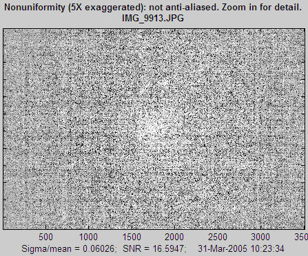
Noise detail, illustrating aliasing. (The actual noise is not as bad as it looks.)
Spot detection (Imatest Master only)
When Spot detection w / threshold (pseudocolor) is selected in the Noise detail popup menu, the pseudocolor display emphasizes dark spots (the type that result from dust on the sensor) and minimizes noise, light spots, and long range density variations. The following webcam image (originally 1600 pixels wide) has two rows of five simulated spots (added by an image editor). Other irregulatities are from the sensor itself..
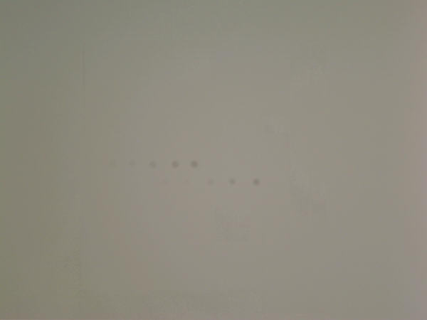
Webcam image with 10 simulated spots (5 in each of 2 rows)
With the standard Pseudocolor contours with colorbar display, the darker spots are clearly visible, but the lighter spots are lost in the overall density variations.
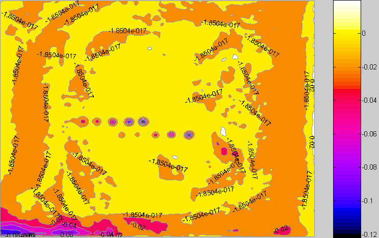
Image with spots: standard pseudocolor display
But they stand out in the Spot detection display. The differences in the algorithms are described below.
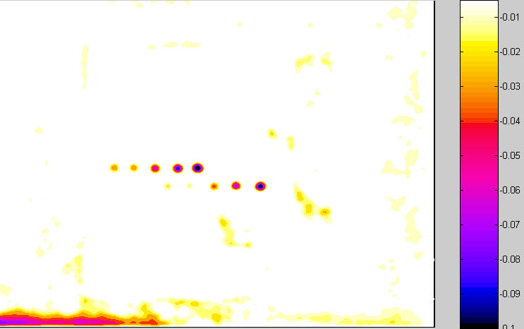
Image with spots: Spot detection display
When Pseudocolor contours with colorbar is selected, the image is normalized to its average level. Then the local variations are calculated by subtracting a highly smoothed version of the image from a moderately smoothed version of the image. This is the same data used for the contours in the Local noise with added contours display, described above.
When Spot detection w / threshold (pseudocolor) is selected, there are several differences.
- The "highly" smoothed version of the image is less aggressively smoothed. This emphasizes local variations more strongly.
- The contour plot has a fixed color map, showing only values between = -0.005 (-0.5%), which is about the threshold of visibility for a spot, and -0.1 (-10%), which is the density for a highly visible spot. All values above -0.005 are displayed as white and all values below -0.1 are displayed as black. The color map for the standard pseudocolor plot is variable, based on the minimum and maximum values of the processed image.
This approach removes much of the interfering detail from the final plot so that spots are clearly visible.
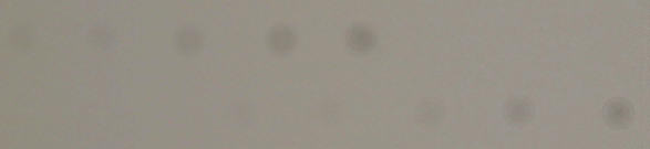
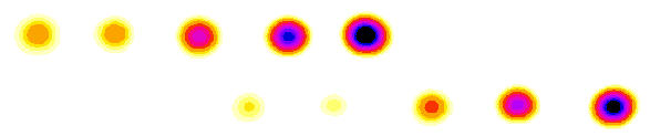
Detail: Simulated spots and Spot detection display
Using Distortion
New in Imatest 2.7.1 Distortion can now analyze square (checkerboard) patterns.
Imatest 2.3.6 Distortion calculations are now more robust, consistent, and less sensitive to region of interest (ROI) selection. The new ROI filtering input option, allows the selection of weak ROI filtering. which produces good results in most cases. A new Radius correction figure has been added (Imatest Master only). |
Distortion
- measures radial lens distortion, an aberration that causes straight lines to curve,
- calculates coefficients for removing it using nonlinear optimization, and
- provides additional information on geometric distortion in digital images.
Distortion calculates the coefficient for correcting distortion using Picture Window Pro, which uses a tangent/arctangent distortion model. A procedure for obtaining approximate Ptlens coefficients is described below.
Lens distortion has two forms, barrel and pincushion, as illustrated below.
Distortion tends to be most serious in extreme wide angle, telephoto, and zoom lenses. It is most objectionable in architectural photography and photogrammetry — photography used for measurement (metrology). It can be highly visible on tangential lines near the boundaries of the image, but it's not visible on radial lines. In a well-centered lens distortion is symmetrical about the center of the image. But lenses can be decentered due to poor manufacturing quality or shock damage.
In the simplest lens distortion model, the undistorted and distorted radii ru and rd (distances from the image center normalized to the center-to-corner distance (half-diagonal) so that r = 1 at the corner) are related by the equation,
ru = rd + k1 rd3 where k1 > 0 for barrel distortion and k1 < 0 for pincushion.
This third-order equation is one of the Seidel Aberrations, which are low-order polynomial approximations to lens degradations. Other aberrations include astigmatism, coma, curvature of field, etc. The third order approximation is sufficient for many lenses, but Imatest also calculates the fifth-order coefficients, which can be more accurate for certain lenses, for example, for the Sigma 18-125mm zoom at 18mm and the Zeiss 21mm f/2.8 Distagon.
ru = rd + h1 rd3 + h2 rd5
Distortion by Paul van Walree is excellent background reading.
To measure distortion, you'll need a rectangular or (preferably) a square grid pattern, which you can create using Test Charts. Print the chart, photograph it, and enter the image into the Imatest Distortion module, as described below.
Instructions
- Test chart. You can use any chart with a square or rectangular grid or a square (checkerboard) pattern.
You can create your own
using
- the Distortion grid or checkerboard pattern the Imatest Test Charts module, or
- the Imatest Screen Patterns module (Distortion grid or Squares (checkerboard)).
The Screen Patterns display, shown on the right, works best with large flat screen LCDs (it's not recommended with CRTs). Click on Screen Patterns on the right the Imatest main window, select Distortion grid or Squares (checkerboard) in the box at the bottom-center, then maximize the window. You can select the number of Horizontal and Vertical lines as well as the line width (in pixels). For best results the pattern should be square.
|
Screen Pattern module for Distortion. |
- A portion of the Test Charts input dialog box is shown on the right, below, with recommended settings:
- Pixels per inch (PPI). 100-300. High resolution isn't necessary because Distortion doesn't measure sharpness.
- Type (grid or checkerboard) selects chart type.
- Horizontal divisions. 10-15 should work for most situations. For extreme distortion, you will either need to use fewer divisions or select an ROI (i.e., crop the image).
- Vertical divisions. Square is recommended in most cases.
- Line width (pxls). Only applies when Type is set to Grid. Typically in the range of .01*PPI to .025*PPI. The printed line should be clear (not pale), but not too thick. The relative line widths in the preview (to the right of the selection boxes) is not to scale. They are (relatively) thicker than in the final image.
The line width should be thick enough to cover at least two pixels in the captured image. Narrower lines may result in errors (Inconsistent number...). For example, suppose your captured image were 640x480 pixels (VGA). The line width (as shown on the right) would be 3 pixels out of a chart width of 1476. In the captured chart, the line width would be 640*(3/1476) = 1.3, inadequate for this small image size, though this chart would be perfectly adequate for 1+ megapixel cameras.
|
Test Charts dialog box for preparing
a file to print the distortion grid. |
- Gamma, and Contrast are turned off for the Grid pattern.
- Print the test chart file. Size isn't critical, but larger is better. (13x19 inches or larger is recommended if your printer can handle it). Matte paper is fine. Handmade charts are acceptable if they're carefully done. The print should be made from an image editor using the saved TIFF file, not the Matlab preview.
- Photograph The chart.
| Be especially careful to avoid glare "hot spots" on chart images. Unlike SFR, where small regions can be selected to avoid hot spots, glare hot spots are likely to interrupt grid lines, which will terminate Distortion analysis. Glare can be especially troublesome with wide angle lenses. To minimize glare we recommend printing Distortion charts on matte surfaces. |
- The chart should be clean. Distortion will terminate if it mistakes spots in the image for lines. If needed, spots can be manually removed using an image editor "clone" function.
- Set exposure compensation to overexpose by one to two f-stops so white areas are light (not middle gray) and line contrast is sufficient.
- The camera should be pointed straight at the chart. (The optical axis of the lens should be normal to the chart surface.) Small amounts of tilt and perspective distortion (convergence of lines; not a lens aberration) are tolerated, but large amounts may cause Distortion to terminate.
- The camera should be set to a low ISO speed to minimize noise. This is especially important for compact digital cameras, where noise can become severe at high ISO speeds.
Good image
 Horizontal and vertical lines should fit between lines in the image for the lines to be detected reliably.
 |
Bad image
 Horizontal line cannot fit between all lines in the image, compromising the reliability of line detection. This image is usable if it is cropped (i.e., a Region of interest is selected).
Imatest versions 2.3.6+ (released May 2007) performs better with images
of this type with ROI filtering set to weak (frequently without cropping), but careful orientation (as shown in the image on the left) is recommended for the most reliable results. |
Save the image. High quality JPEG format is preferred because it preserves EXIF data in a format Imatest can read. There is no need for RAW quality.
Resize the image? Because Matlab uses double precision for most math operations, each 24-bit color pixel requires 24 bytes. A 6.3 megapixel image can take 151 megabytes of memory (ouch). This can slow down computations in computers that don't have gobs of memory. (It can even bog down computers with 512k of memory.) We are looking into solving this problem. In the meantime we recommend resizing images to about 1000 pixels wide in an image editor. (Any editor will do.) Resizing has no effect on the results.
Launch Imatest. Click on Distortion.
Very large files (height x width x colors over 40 MB) may cause memory overflow problems. Files over 40 or 80 MB can be automatically reduced 1/2x linearly (using 1/4 the memory). Click Settings, Options and Settings... (in the Imatest main window) and make the appropriate setting in LARGE FILES (Light Falloff, Distortion).
Open the image file.
| Batch mode This module can operate in batch mode in Imatest Master, i.e., it can read multiple input files. All you need to do is select several files using the standard Windows techniques of shift-click or control-click. There are three requirements for the files. |
| They should (1) be in the same folder, (2) have the same pixel size, and (3) be framed identically. |
| The input dialogs (cropping (if applicable), settings, and save) are the same for the first run as for standard non-batch runs. Additional runs use the same settings as the first run. Since no user input is required they can run extremely fast. |
| If the order of the files in a batch runs is different from the selection order, click Settings, Options and Settings... (in the Imatest main window) and change the setting in Batch run order. |
| One caution: Imatest can slow dramatically on most computers when more than about twenty figures are open. For this reason we recommend checking the Close figures after save checkbox, and saving the results. This allows a large number of image files to be run in batch mode without danger of bogging down the computer. |
|
Crop the image (select the ROI) if needed using the usual clicking and dragging technique. Cropping may be helpful if horizontal or vertical lines are not entirely within the ROI (region of interest), though Imatest 2.3.6+ often works well in such cases. An example is shown below in the section on Severe distortion. Click outside the the image to select the entire image. You can select either a grid pattern or a single line, which is useful in patterns such as the ISO 12233 chart, which contains two lines suitable for Distortion: one nearly vertical and one nearly horizontal (both slightly tilted). One of them is illustrated below. Make sure to leave some breathing room around the line. In selecting the crop for grid patterns (or deciding not to crop) try to choose a crop where no lines cross the crop boundaries, i.e., are partly inside and partly outside. The horizontal (well... sort of) line at the bottom right of the "Bad" image above is caused Distortion to terminate in Imatest versions earlier than 2.3.6, but is very likely to work will with 2.3.6+.
Three cropping (ROI selection) options are available by clicking Settings, Options and Settings... in the Imatest main window. These include
| Never crop. |
| Select crop by dragging cursor. Ask to repeat crop for same sized image. |
| Select crop by dragging cursor. Do not ask to repeat crop. |
Although the first option (Never crop...) was the default in early version of Distortion, the second option (Select crop by dragging cursor. Ask to repeat crop for same sized image), which is similar to the ROI selection in SFR, may be preferred in many cases.
The input dialog box, shown below, appears. Title defaults to the file name; you may change it if needed. The most important choice is the algorithm that detects pattern location. Figures can be selected in the Plot box on the right. Plot intersection points, Plot radius correction, and Display corrected image appear in Imatest Master only.
Distortion input dialog box
- Pattern
- For grid patterns, choose Grid.
- For lines, choose Single line (some interference). This is the appropriate choice for the usable lines in the ISO-12233 pattern. "Interference" refers to extra detail that may be present near the line (lettering, etc.) This choice will work for lines near the boundaries of a grid pattern. An example from an ISO-12233 chart is shown below.
- For square/checkerboard patterns, choose Squares (checkerboard). This pattern, introduced with Imatest 2.7.1, may be slightly more robust than the grid.
- Calculate line display using selects the formula for plotting the corrected lines. Useful for comparing the different algorithms. Choices are 3rd order (coefficient k1 , below), 5th order (coefficients h1 and h2 , below), and PW Pro (Picture Window Pro) tan/arctan (coefficient p1 , below).
- Decentering calculation is described below. It is optional because it takes extra time. It can only be selected for the Grid pattern. It the box is unchecked, distortion is assumed to be symmetrical around the geometric center of the image.
- ROI filtering When set to Strong, this setting filters out ROIs that might cause Distortion to crash — in Imatest versions earlier than 2.3.6. We recommend setting ROI filtering to Weak since many boundary conditions that formerly crashed Imatest now work well.
- Plot area. Selects which plots to produce.
- Plot distortion figure selects the main distortion figure.
- The Plot intersection points and Detect points outside crop checkboxes are described below. If the first of them is checked, another figure is produced. They only work with the Grid pattern.
- Plot radius correction is described below.
- Display corrected image creates an additional figure with the corrected image calculated with the algorithm selected in Calculate line display using, above. It is most valuable for highly distorted lenses where the input image has been cropped. Choices are never, crop only (the default), and always. An example is shown below in the section on Severe distortion.
Click OK. The calculations are performed, and the results figure(s) described in Results appears. You can zoom in by clicking on (and highlighting) the magnifier icon  , then clicking on portions of the image of interest, as shown below. The detected points on the image are shown as red squares. The straightened line is drawn in magenta. Double-clicking restores the entire image.
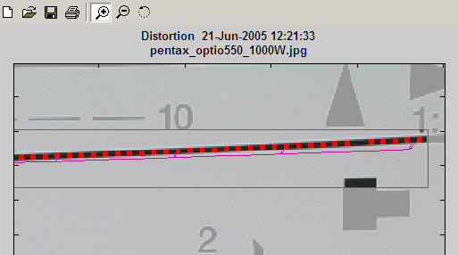
An enlarged portion of the results figure.
When the calculations are complete the Save dialog box appears. The default directory is subdirectory Results in the data file directory. You can change to another existing
directory,
but new results directories must be created outside of Imatest— using
a utility such as Windows Explorer. (This is a limitation of this
version
of Matlab.) The selections are saved between runs.
You can examine the output figures before you check or uncheck
the boxes. Select the items you wish to save, then click Yes or No. File names (where filename is the input file name):
[filename]_distortion.png
[filename]_corrected.png (only if displayed)
[filename]_intersections.png
[filename]_radius_corr.png
[filename]_summary.csv
[filename].xml
|
Save results dialog box |
The root file name ([filename], above) defaults to the image file name, but can be changed using the Results root file name box. Be sure to press enter. Checking Close figures after save is recommended for preventing a buildup of figures (which slows down most systems) in batch runs.
The CSV and XML files contain EXIF data, which is image file metadata that contains important camera, lens, and exposure settings. By default, Imatest uses a small program, jhead.exe, which works only with JPEG files, to read EXIF data. To read detailed EXIF data from all image file formats, we recommend downloading, installing, and selecting Phil Harvey's ExifTool, as described here.
Results
Main figure
An example of Distortion output is shown below for the Sigma 18-125 mm f/3.5-5.6 DC lens (designed for APS-C-sized sensors, such as the Canon EOS-10D, 20D, Digital Rebel, Nikon D100, D70, etc. The Sigma is an excellent lens — a bargain — except for its autofocus. Mine doesn't autofocus as reliably as Canon lenses, but it works beautifully on manual. The autofocus problem is plainly visible when working with the distortion chart.
Main figure showing modest pincushion distortion
The Sigma has modest amounts of pincushion distortion at 125 mm and barrel distortion at 18mm, its widest angle setting. Corrected vertical lines are deep magenta; horizontal lines are blue. Results displayed below the image on the left include.
- TV Distortion from the SMIA specification, §5.20. Referring to the image on the right,
SMIA TV Distortion = 100( A-B )/B ; A = ( A1+A2 )/2
The box on the right is described in the SMIA spec as "nearly filling" the image. Since the test chart grid may not do this, Distortion uses a simulated box whose height is 98% that of the image. Note that the sign is opposite of k1 and p1. SMIA TV Distortion > 0 is pincushion; < 0 is barrel.
|
SMIA TV Distortion |
 SMIA vs. traditional TV distortion SMIA vs. traditional TV distortion
Thanks to Mark Butterfield for pointing out that SMIA's distortion definition differs from the traditional TV industry definition by a factor of two. The traditional definition is shown in the illustration on the right, which has been adapted from the publication "Optical Terms," published by Fujinon. The same definition appears in "Measurement and analysis of the performance of film and television camera lenses" published by the European Broadcasting Union (EBU). SMIA TV distortion is double the traditional TV distortion definition.
Imatest will continue to use the SMIA definition, which has been widely adopted in the mobile imaging industry. We prefer it because it is self-consistent. In the traditional definition, TV distortion is the change (Δ) in the center-to-top distance divided by by the bottom-to-top distance. In the SMIA definition, both A and B are bottom-to-top distances. |
|
Picture Window Pro uses a tangent/arctangent model of distortion, which works well for a variety of lenses, including fisheyes.
ru = tan(10 p1 rd )/ (10 p1 ) ; h1 > 0 (barrel distortion)
ru = tan-1(10 p1 rd )/ (10 p1 ) ; h1 < 0 (pincushion distortion)
Where p1 is the correction coefficient. Using Taylor series, we can show that it is similar to the third-order model,
tan(x) = x + x3/3 +2x5/15 + ... ; tan-1(x) = x - x3/3 + x5/5 - ... ( x2 < 1) ;
ru = x + 100 p12x3/3 + ... (barrel); ru = x - 100 p12x3/3 + ... (pincushion) ,
k1 ≈ sign( p1)*100 p12/3 for small values of k1 and p1. k1 and p1 diverge for large values.
The plot includes arrows that illustrate the change in radius when distortion is corrected. Distortion was too low on the above plot to make the arrows visible. They are illustrated in the plot below for a large amount of simulated barrel distortion. You can try different line display calculations to see the difference.
Main figure with extreme (simulated) pincushion distortion, illustrating arrows.
Here is an example of results from an ISO 12233 test pattern, which contains two lines suitable for measuring distortion. They work but they're not ideal: they would be better if they were thinner and closer to the image boundaries. This camera has a modest amount of pincushion distortion. A zoom of a portion of the selected area is shown above.
Decentering (Imatest Master only)
Distortion is normally centered around the geometric center of the image, but it may be decentered due to poor lens manufacturing quality or shock (i.e., dropping the lens). Decentering can appear as a shift in the center of distortion symmetry or as asymmetrical MTF (sharpness) measurements in SFR. Distortion calculates decentering if Decentering calculation is checked in the Input dialog box and |k1| > 0.01. (k1 is the third-order coefficient.) If |k1| is smaller, distortion is insignificant (and difficult to see); hence decentering has no meaning.
Decentering is reported by the radius (in units of the distance from the image center to the corner) and angle in degrees of the center of distortion symmetry. It is illustrated in the simulated pattern below. The geometrical center of the image is indicated by a pale blue +. The center of the decentered distortion is indicated by bold red X.
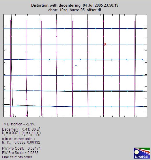
Severe distortion: Corrected image figure
Images from optical systems with severe distortion (fisheye lenses, etc.) often need to be cropped so Distortion can detect vertical and horizontal lines. (See good/bad images, above.) The figure below illustrates an inexpensive fisheye lens. The crop area, shown in the middle, is displayed with full contrast; the area outside the crop has reduced contrast.
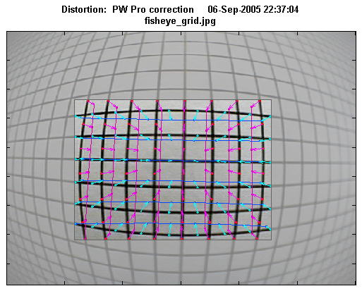
This figure does not show the corrected grid image outside the crop. The different correction formulas (3rd order polynomial, 5th order polynomial, or tangent/arctangent) can only be compared inside the crop area, where optimum coefficients have been calculated. They don't look very different in this region.
If Display corrected image in the input dialog box (Imatest Master only) is set to crop only or Always, the corrected image (shown below) is displayed. (The extreme corners are omitted for large amounts of barrel distortion). This figure is not perfect. It is calculated using a simple, fast algorithm that omits some pixels on the left and right. A semicircular "fingerprint" pattern" appears in their place. But is good enough to clearly illustrate the performance of the correction algorithm. (Another option, always - interpolated (SLOW!), produces a fine image without any gaps, but is too slow to be recommended.)
In this case, some residual barrel distortion is visible in vertical grid lines on the left and right and some residual pincushion distortion is visible in the horizontal grid lines on the top and bottom. The average correction is quite good. The tangent/arctangent algorithm (used in Picture Window Pro) gives slightly better results for this image than the 5th order polynomial (which is normally most accurate), and much better than the 3rd order polynomial.
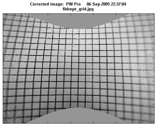
This image has some perspective distortion: vertical convergence of lines. This results from the way the camera was pointed when the image was captured. It is not a lens aberration.
Intersection figure (Imatest Master only)
Checking Plot intersection points in the input dialog box displays a second figure that contains intersection points (line crossings) designated by "+," "T," or "L." "+" intersection points are inside the pattern; "T" points are on the boundaries (top, bottom, and sides), and "L" points are on the corners.
The image should be cropped so that only "+" intersection points (line crossings) are present inside the crop. Imatest doesn't like boundaries with "T" or "L" patterns inside the crop. To detect such patterns, they must be outside the crop (as shown above) and Detect points outside crop must be checked in the input dialog box. These points are not used in the for calculating distortion coefficients.
If the image contains letters or material unrelated to the the pattern, it should be edited out using an image editor. Picture Window Pro has a particularly convenient means of creating a rectangular mask for this purpose.
The (x,y) coordinates of the displayed points are included in the optional .CSV and XML output files. There coordinates can be used for further analysis of geometric distortion.
Thanks is due to Karl-Magnus Drake of the National Archives of Sweden for suggesting this figure.
Radius correction figure (Imatest Master only)
Checking Plot radius correction in the input dialog box displays a figure that contains detailed distortion/radius correction information, which can be useful for analyzing images like the one on the right, which has barrel distortion near the center but tends towards pincushion near the corners.
The upper plot shows the distortion-caused change in radius Δr (normalized to the center-to-corner distance, i.e., the half-diagonal) as a function of the distorted (input) radius r(distorted) = rd.
Δr = r(corrected) - r(distorted) = ru - rd
where r(corrected) = ru is the corrected ( undistorted) radius. Δr is a function of the scaling (i.e., magnification) of the corrected image, |
Image showing complex ("wave") distortion: barrel near
center; pincushion near corners. |
The bold solid lines —— in the upper plot show Δr for no scaling, i.e., for the straight correction formulas: ru = rd + k1 rd3 (3rd order; blue); ru = rd + h1 rd3 + h2 rd5 (5th order; green); or the arctan/tan equations (red). With these equations Δr tends to increase as a function of r(distorted), i.e., it tends to be largest near the image corners.
The dashed lines - - - - show Δr when ru (the corrected image) is scaled for no shift (Δr = 0) at the image corners (rd = 1). The scaling factor is shown in the Legend box, which also shows the error function (described in the Algorithm; different for the 5th order calculation) and the number of iterations.
The upper plot is difficult to relate to the perceived distortion type (pincushion or barrel); the only difference between the solid and dashed lines is the scaling factor (image magnification). The lower plot, which contains Curvature and Distortion measurements (explained in the green box below) is directly related to the distortion type .
| Equations for distortion and curvature |
The standard distortion equations— ru = rd + k1 rd3 (3rd order), ru = rd + h1 rd3 + h2 rd5 (5th order), or the arctan/tan equations— do not give a clear picture of whether distortion takes the barrel or pincushion form. And to complicate matters, some images like the one above have barrel distortion at some radii and pincushion at others.
The key to determining the type of distortion is to recall that radius ru is the position of a point, its derivative dru /drd is the slope, and its second derivative d 2ru /drd2 is the curvature— local curvature, which is a function of radius r closely related to distortion.
It is instructive to look at the first and second derivatives of the 3rd and 5th order equations.
3rd order: dru /drd = 3 k1 rd2 ; d 2ru /drd2 = Curvature = 6 k1 rd .
5th order: dru /drd = 3 h1 rd2 + 5 h2 rd4 ; d 2ru /drd2 = Curvature = 6 h1 rd + 20 h2 rd3 .
The problem with Curvature as defined here is that it tends to be proportional to r (it's exactly proportional for the 3rd order equation). To get a more consistent measurement, we define Distortion as Curvature divided by r.
Distortion = Curvature/r = 6 k1 (3rd order) = 6 h1 + 20 h2 rd2 (5th order)
Distortion is a single number for the 3rd order case. Distortion and Curvature is only visible in lines that have a tangential component. Tangential edges are illustrated in the page on Chromatic Aberration. |
|
Curvature ( d 2ru /drd2 ) and Distortion (Curvature/r) are plotted as dashed ( - - - ) and bold solid —— lines, respectively, in the lower plot.
Interpretation:
Positive Distortion (and Curvature) represents local barrel distortion;
Negative represents local pincushion distortion.
In the example above, distortion goes from barrel to pincushion around rd = 0.8 (the diameter at the sides of the image). This is visible near the corners, where the (barrel) curved lines straighten out.
The blue lines (3rd order equation) are the simplest but least accurate approximation to distortion. The 5th order equation (red lines), which has two parameters (h1 and h2 ), is more accurate. If the 3rd and 5th order curves are close, the 3rd order curve is sufficient. In the above example, which is not typically, they are very different; the third order equation is completely inadequate. The arctan/tan equation is also characterized by a single parameter. It behaves differently from the 3rd order equation for large Δr.
The 3rd order distortion value in the figure is a constant solid blue blue equal to 6 k1 .
Links
Real-Time Lens Distortion Correction by Michael R. Bax (of Stanford) contains the standard distortion equation, ru = rd (1 + k1 rd2) and its inverse (more complex).
Distortion by Paul van Walree, who also has excellent descriptions of several of the lens (Seidel) aberrations and other sources of optical degradation.
Lens aberrations, including distortion, are discussed in pages from James R. Graham of the U.C. Berkeley Astronomy Department, based on Applied Optics & Optical Engineering, Vol XI by J. C. Wyant & K. Creath, which goes into real depth. Worth checking out if you're mathematically inclined.
Optical Metrology Center A UK consulting firm specializing in photographic metrology. (Site must be viewed with Internet Explorer.) They have a large collection of interesting technical papers emphasizing distortion and 3D applications, for example, Extracting high precision information from CCD images.
PTlens is an excellent program for correcting distortion. It uses the equation from Correcting Barrel Distortion by Helmut Dersch, creator of Panorama Tools, who states,
Photogrammetry is the science of making geometrical measurements from images. George Karras has sent me some interesting links with material relevant to Imatest development: http://www.vision.caltech.edu/bouguetj/calib_doc/ | http://nickerson.icomos.org/asrix/index.html.
The correcting function is a third order polynomial. It relates the distance of a pixel from the center of the source image (rsrc) to the corresponding distance in the corrected image (rdest) :
rsrc = ( a * rdest3 + b * rdest2 + c * rdest + d ) * rdest
The parameter d describes the linear scaling of the image. Using d=1, and a=b=c=0 leaves the image as it is. Choosing other d-values scales the image by that amount. a,b and c distort the image. Using negative values shifts distant points away from the center. This counteracts barrel distortion... The internal unit used for rsrc and rdest is the smaller of the two image lengths divided by 2.
This equation drives me nuts! rsrc and rdest are reversed from the equations on this page; it only goes up to fourth power (when you include rdest outside the parentheses; third power if you don't); and it has even order terms (a and c) when the theory implies that distortion can be modeled with odd terms only. Give me a higher order term (h * rdest4 ) and dump a * rdest3 and c * rdest. But nonetheless it works pretty well.
| Mike Collins has posted a technique for finding PTlens parameters on a dpreview.com forum. I haven't checked to verify it. Briefly, |
| 1) take a shot of the grid pattern and run Imatest distortion. Note the k1 (which is the r^3) parameter. |
| 2) divide my magic number = -3.397. This result is now used as the b (r^3) parameter in Ptlens. |
| 3) Edit the profile file used in Ptlens to include this new lens. Use the bodies multiplier, lens name, focal length, a, b, c ( make a and c 0.000000; and b from calculation in 2) ). More details on the post. |
|
Modeling distortion of super-wide-angle lenses for architectural and archaeological applications by G. E. Karras, G. Mountrakis, P. Patias, E. Pets
| Algorithm for calculating correction coefficients. |
The coefficients of the standard distortion equations are calculated using nonlinear optimization that straightens the lines (minimizes their curvature). The equations are
ru = rd + k1 rd3 (3rd order) rd is the distorted (input) radius; ru is the undistorted (output) radius.
ru = rd + h1 rd3 + h2 rd5 (5th order)
ru = tan(10 p1 rd )/ (10 p1 ) ; h1 > 0 (arctan/tan; barrel distortion)
ru = tan-1(10 p1 rd )/ (10 p1 ) ; h1 < 0 (arctan/tan; pincushion distortion)
The optimizer
- finds the average locations of vertical and horizontal lines in the image,
- scans between the lines to find (x,y) locations on the lines (and if there is room, scans lines that intersect the image boundaries),
- finds polynomial fit for each line,
- minimizes the sum of squares of the second order polynomial coefficients, which are the line curvatures. For the 5th order case the optimizer minimizes the sum of squares of the second and fourth order polynomial coefficients— a slightly different error function from the 3rd order and arctan/tan cases.
Since optimization is performed only to straighten curved lines, this algorithm is relatively insensitive to perspective distortion and small amounts of camera misalignment. |
|
Using Print Test
Measure print quality factors: color response, tonal response, and Dmax
Introduction
Imatest Print Test
measures several of the key factors that contribute to photographic print quality,
- Color response, the relationship between pixels in the image file and colors in the print,
- Color gamut, the range of saturated colors a print can reproduce, i.e., the limits of color response,
- Tonal response, the relation between pixels and print density, and
- Dmax, the deepest printable black tone: a very important print quality factor,
using a print of a test pattern scanned on a flatbed scanner. No specialized equipment is required. You can observe response irregularities by viewing the test print, but you need to run Print Test to obtain detailed measurements of the print's color and tonal response.
The essential steps in running Print Test are
- Assign a profile to the test pattern, if needed.
- Print the test pattern, noting (as applicable) the printer, paper, ink, working color space, ICC profile, rendering intent, color engine, and miscellaneous software settings.
- Scan it on a flatbed scanner, preferably one that has been profiled. Best results are obtained by scanning it next to a step chart such as the Koda Q-13.
- Run Imatest Print test.
Color quality is a function of gamut— the range of saturated colors a print can reproduce, as well as overall color response— the relationship between file pixels and print color. Tonal quality is strongly correlated with Dmax— the deepest attainable black tone, as well as the tonal response curve. Prints usually appear weak in the absence of truly deep black tones.
The test pattern, shown (reduced) on the right, was generated using the HSL color representation.
- H = Hue varies from 0 to 1 for the color range R→ Y→ G→ C→ B→ M→ R (horizontally across the image on the right). (0 to 6 is used in the Figures below for clarity.)
- S = Saturation = max(R,G,B)/min(R,G,B). S = 0 for gray; 1 for the most saturated colors for a given Lightness value.
- LHSL = Lightness = (max(R,G,B)+min(R,G,B))/2. (The HSL subscript is used to distinguish it from CIELAB L.) L = 0 is pure black; 1 is pure white. The most visually saturated colors occur where LHSL = 0.5.
The key zones are,
- S=1. A square region consisting of all possible hues (0 ≤ H ≤ 1) and lightnesses (0 ≤ LHSL ≤ 1), where all colors are fully saturated (S = 1), i.e., as saturated as they can be for the Lightness value.
- L=0.5. A rectangular region consisting of all possible hues (0 ≤ H ≤ 1) and saturation levels (0 ≤ S ≤ 1) for middle Lightness (LHSL = 0.5), where colors are most visually saturated.
- Two identical monochrome tone scales, where pixel levels vary linearly, 0 ≤ {R=G=B} ≤ 1.
The zones labelled K, Gry, and W are uniform black (pixel level = 0), gray (pixel level = 127), and white (pixel level = 255), respectively.
Detailed instructions
- The printer test patterns are located in the images subfolder of the Imatest installation folder. They can also be downloaded from the following links: Print_test_target.png (no embedded profile), Print_test_target_sRGB.tif , Print_test_target_Adobe.tif, Print_test_target_WGRGB.tif (embedded profiles as indicated in the file name). These patterns all contain the same data; only the profile tag differs. [I was unable to save embedded profiles in PNG files with any of my editors, so I used LZW-compressed TIFF. (I found a small error when using maximum quality JPEGs.)]
| Assigning a profile: To explore the effect of working color space on print quality you may want to change the ICC profile of the test image without changing the image data. |
In Photoshop: Click Image, Mode, Assign Profile...
|
In Picture Window Pro: Click Transformation, Color, Change Color Profile... Set Change: (the bottom setting) to Profile Setting Only. |
- Open a test pattern in an image editor, preferably an ICC-aware image editor such as Photoshop or Picture Window Pro with color management enabled. For most printer testing I recommend Print_test_target_Adobe.tif, which has an embedded Adobe RGB (1998) profile, but patterns with other color spaces are also of interest. Print test lets you see the effect of printing with different color spaces.
- Print the pattern, approximately 6.5x10 inches (16x25 cm), from your image editor. Carefully record the paper, ink, working color space, ICC profile, rendering intent, and printer software settings. I recommend running a nozzle check before making the print— just make sure everything is OK.
- Scan the print on a flatbed scanner at around 100 to 150 dpi. The scanned image should be no larger than about 1500 pixels high. Higher resolution is wasted; it merely slows the calculations. The pattern must be aligned precisely (not tilted). The scanner's auto exposure should be turned off and ICC Color Management should be used if possible.
On the Epson 3200 flatbed scanner, I click on the Color tab in the Configuration dialog box, then select ICM. Source (Scanner): is either be EPSON Standard or a custom scanner profile. Target: should be one of the three profiles recognized by Print test: sRGB (small gamut; comparable to CRTs), Adobe RGB (1998) (medium gamut; comparable to high quality printers), or Wide Gamut RGB (larger gamut than any physical device). Since the Epson standard profile, which represents the scanner's intrinsic response, has a large gamut (between Adobe and Wide Gamut RGB, according to ICC Profile Inspector), and since the measured printer gamut is bounded the gamut of the working color space, a moderate to large gamut color space should be chosen for best accuracy. I recommend Adobe RGB. The profile is not embedded in the output file; you'll need to remember it: it can be part of the file name.
- Save the scan with a descriptive name. TIFF, PNG, or maximum quality JPEG are the preferred formats. A reduced scan of a print made on the Epson 2200 printer with Epson Enhanced Matte paper and the standard Epson ICC profile is shown above. Colors are somewhat more subdued than glossy, semigloss, or luster papers.
- Accuracy is improved if you scan a Q-13 or equivalent reflective step chart next to the print (shown on the right of the above image), then run Stepchart. When the run is complete, check the box labelled "Save Print test calibration data" in the Save Q-13 Stepchart Results window. This saves the tonal response and Dmax calibration data, even if you click No to Save Q-13 Stepchart results? This only needs to be done once for a set of scans made under identical conditions. This optional step improves the accuracy of the tonal response and Dmax.
| Scanner settings and performance verification |
 For the Epson 3200 flatbed scanner, the Configuration dialog box, shown on the right, is opened by clicking Configuration... in the main window. If you have a trustworthy custom profile for your scanner, you should enter it in the Source (Scanner): box. The Epson Standard (default) profile is shown. For the Epson 3200 flatbed scanner, the Configuration dialog box, shown on the right, is opened by clicking Configuration... in the main window. If you have a trustworthy custom profile for your scanner, you should enter it in the Source (Scanner): box. The Epson Standard (default) profile is shown.
If the custom profile is not visible, go to Control Panel, double-click on Scanners and Cameras, right-click on your flatbed scanner, click Properties, then click on the Color management tab. Click Add... then select the custom profile. (A lotta steps!)
Target: contains the output profile for the scan. Adobe RGB is recommended in most cases because its gamut exceeds that of most high quality printers: sRGB (the default) may not be sufficient. Make sure to select the same Color space for the scanner in the Print test input dialog box. Note: this profile is not embedded in the scanner output. This is a deficiency in the Epson scanner software: almost a bug (though a common bug; it appears in many cameras and raw converters.). You need to remember the profile and embed it in the file without changing the image data. See Assigning a profile, above. |
| Is the scanner gamut large enough? The default color space of the Epson 3200 scanner (for reflected images) is shown on the right. Its gamut is larger than sRGB and Adobe RGB (1998), shown below. The images are from Profile inspector, a nice little free program downloadable from Color.org, the official site of the ICC (the committee that gives us color management and all that). It's not the most convenient program— I had to combine the R, G, B, and White points. But it does the job. The scanner and Adobe RGB (1998) should cover the gamuts of most high quality printers. |
 |
Scanner color response: Because Print test results are filtered by the scanner's color response, it's a good idea to verify it using Colorcheck. The response of the Epson 3200 with Epson's default ICC profile, shown below, is very good; comparable to the best digital cameras. For the best accuracy you should profile your scanner using one of several available software packages. |
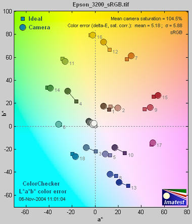 |
Scanner profiling on a budget from Photographical.net has a nice introduction to the process. Part 2 describes a promising free program called IPhotoMinusICC. (I has lots of poorly-documented options. I tried it and didn't get good results. I didn't take the time to figure out where I went wrong.) There are also several commercial programs of interest:
Profile Mechanic - Scanner from the creators of my favorite image editor, Picture Window Pro. Works with IT8, GretagMacbeth ColorChecker, and other charts.
Profile Prism
MonacoEZColor
|
- Run Imatest. Select the Print test module. Crop the image so a small white border appears around the test pattern. If you scanned a Q-13 chart beside the test chart, be sure to omit it from the crop. After you've cropped the image, the Print test input dialog box, shown below, opens. Help opens a browser window containing a web page describing the module. The browser window sometimes opens behind other windows; you may need to check if it doesn't pop right up.
Two color spaces, both of which default to sRGB, need to be entered manually because Print test does not recognize embedded ICC profiles. (And many scanners don't bother to embed them in their output.)
- Specify the (original) working color space used to print the target. This space is used in the La*b* plots below to generate curves representing the color space for various L (lightness) and S (saturation) levels. These lines are used to compare the actual and ideal color responses.
- Specify the color space used for the scanner output. In the Epson 3200, it is specified Configuration... dialog box, described above.
The two checkboxes in the Plot box select figures to display. (La*b* plots are always displayed.) The HSL contour plots, illustrated below, are derived from RGB values whose meaning is dependent on the color space. They are highly detailed, but lack the absolute color information contained in the La*b* plots. The CIE xy plot is a CIE 1931 chromaticity plot of the gamut (for L = 0.5, S = 0 to 1 in steps of 0.2, and 0 ≤ H ≤ 1). It is familiar, but less readable and less perceptually uniform than the La*b* plot.
Print Test results are filtered by the color space of the scanned file. The Windows default is sRGB, which has a limited gamut. For best results you should scan to a color space with a larger gamut— comparable to your printer. I recommend Adobe RGB (1998). At present I don't recommend Wide Gamut RGB, which hs a gamut far larger than any printer you're likely to encounter.
Results
Results below are for Epson 2200 printer with Ultrachrome inks, Premium Luster paper, and the standard 1440 dpi Epson profile. The sRGB test file was used to make the print.
Density
The first Figure contains the grayscale density response and the maximum density of the print, Dmax, where density is defined as –log10(fraction of reflected light). The value of Dmax (2.24) is the average of the upper and right black areas. This value is excellent for a luster (semigloss) paper. Matte surfaces tend to have lower values, typically around 1.8.
The upper plot shows print density as a function of log10(original pixel level (in the test pattern)/255). This corresponds to a standard density-log exposure characteristic curve for photographic papers. The blue plot is for the upper grayscale; the black plot is for the lower-right grayscale. Somewhat uneven illumination is evident. The print density values are calculated from Q-13 calibration curve (lower right). The thin dashed curves contain –log10(pixel levels).
The lower left curve is the characteristic curve (print vs. original normalized pixel level) on a linear scale.
The lower right curve is the results of the (separate) Q-13 calibration run used to calibrate Dmax and the density plot.
S=1 La*b* Gamut map
CIELAB is a relatively perceptually uniform device-independent color space, i.e., that the visible difference between colors is approximately proportional to the distance between them. It isn't perfect, but it's far better than HSL (where Y, C, and M occupy narrow bands) or or the familiar CIE 1931 xyY color space, where gamuts are represented as triangles or hexagons inside the familiar horseshoe curve and greens get far more weight than they should.
In CIELAB, colors can be represented on the a*b* plane. a* represents colors ranging from cyan-green to magenta, and b* represents colors from blue to yellow. a* = b* = 0 is neutral (zero chroma). L is a nonlinear function of luminance (where luminance ≈ 0.30*Red + 0.59*Green + 0.11*Blue). The colors of the a*b* plane are represented roughly in the background of the Figure below.
The S = 1 CIE La*b* gamut map below displays cross sections of the La*b* volume representing the printer's response to test file HSL lightnesses (LHSL) of {0.1, 0.3, 0.5, 0.7, and 0.9} where S = 1 (maximum saturation). These values correspond to near black, dark gray, middle gray, light gray, and near white. Printer gamuts are represented as thick, solid curves. The corresponding values for the original color space— the color space used to print the pattern— are displayed as dashed curves.
Note: The L-values below refer to LHSL in the test file, not CIELAB L.
Although this display contains less information than the HSL map (below), the results are clearer and more useful. CIELAB gamut varies with lightness: it is largest for middle tones (LHSL = 0.5) and drops to zero for pure white and black. This is closer to the workings of the human eye than HSL representation.
The petal-like dotted concentric curves are the twelve loci of constant hue, representing the six primary hues (R, Y, G, C, B, M) and the six hues halfway between them.. They follow different curves above and below L = 0.5. The circles on the solid curves show the measured hues at locations corresponding to the twelve hue loci. Ideally they should be on the loci. The curves for L = 0.5 (middle gray) are outlined in dark gray to distinguish them from the background.
The hexagonal shape of the gamuts makes it easy to judge performance for each primary. The measured (solid) shape should be compared to the ideal (dotted) shape for each level. Weakness in magenta, blue, and green is very apparent, especially at L = 0.5 and L = 0.7. But the gamut is excellent for L = 0.3.
L=0.5 La*b* Saturation map
L=0.5 Saturation results are also well suited for display on the CIELAB a*b* plane. Gamuts are shown for 0 ≤ S ≤ 1 in steps of 0.2. As in the the S=1 La*b* Saturation map, the dotted lines and shapes are the ideal values (the color space used to print the pattern) and the solid shapes are the measured values. If the scanner color space is different from the original color space (used to print the target), the scanner color space is slown as thin light dotted lines, barely visible in the image below.
Gamut is excellent for S = 0.2 (brown curve) and 0.4 (red curve). But compression becomes apparent just beyond S = 0.4 for magenta and blue and at S = 0.6 (green curve) for green and cyan, where the printer starts to saturate. Increasing S above these values doesn't increase the print saturation: in fact, saturation decreases slightly at S = 1. This is the result of limitations of the Epson 2200's pigment-based inks and the workings of the standard Epson ICC profile. The good performance for relatively unsaturated colors (S ≤ 0.4) is extremely important: skin tones and other subtle tones should reproduce very well on the Epson 2200.
With Gamut maps, differences between printers, papers, and profiles are immediately apparent. These differences are far more difficult to visualize without Imatest Print test because each image has its own color gamut. One image may look beautiful but another may be distorted by the printer's limitations.
L=0.5 xy Saturation map
L=0.5 Saturation results can also be displayed in the familiar CIE 1931 xy chromaticity chart. As with the La*b* plot above, Gamuts are shown for 0 ≤ S ≤ 1 in steps of 0.2. As in the the S=1 La*b* Saturation map, the dotted lines and shapes are the ideal values (the color space used to print the pattern) and the solid shapes are the measured values.
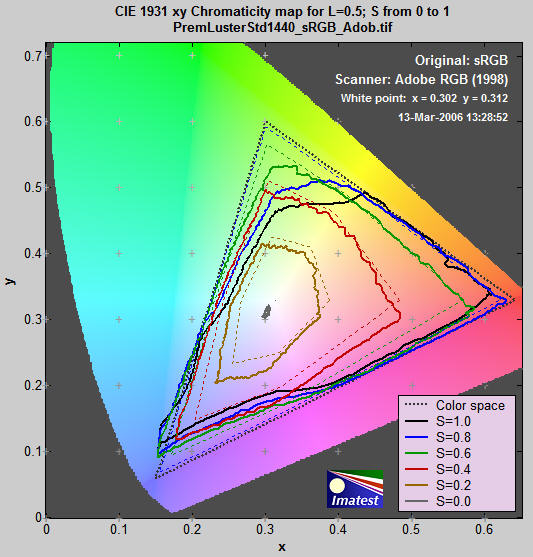
Gamut is excellent for S = 0.2 (brown curve) and 0.4 (red curve). But compression becomes apparent just beyond S = 0.4 for magenta and blue and at S = 0.6 (green curve) for green and cyan, where the printer starts to saturate. Increasing S above these values doesn't increase the print saturation: in fact, saturation decreases slightly at S = 1. This is the result of limitations of the Epson 2200's pigment-based inks and the workings of the standard Epson ICC profile. The good performance for relatively unsaturated colors (S ≤ 0.4) is extremely important: skin tones and other subtle tones should reproduce very well on the Epson 2200.
HSL contour plots
The HSL contour plots that follow display color response in great detail, but don't contain absolute color information. For that you need the La*b* or CIE 1931 xy plots described above. They work best when the same color space is used to print and scan the target. For these plots to be displayed, Display HSL coutour plots must be checked in the Print test input dialog box.
S=1 HSL Saturation plot
The S=1 Figures are for region 1, which contains all possible hues (0 ≤ H ≤ 1) and lightnesses (0 ≤ LHSL ≤ 1) for maximum HSL saturation (S = 1).
The HSL Saturation plot shows the saturation levels. If the print and scanner response were perfect, S would equal 1 everywhere. Weak saturation is evident in light greens and magentas (L > 0.5). Strong saturation in darker regions, roughly 0.2 ≤ L ≤ 0.4, could indicate that it might be possible to create a profile with better performance in the light green and magenta regions. Weak saturation in very light (L>0.95) and dark areas (L<0.1) is not very visible.
S=1 HSL Lightness plot
The ideal lightness plot would display uniformly spaced horizontal lines from 0.9 near the top to 0.1 near the bottom. (It generally doesn't go much below 0.1 because of the effects of Dmax and gamma.This plot shows relatively uniform response except for blues with L between 0.3 and 0.6, which appear darker than they should.
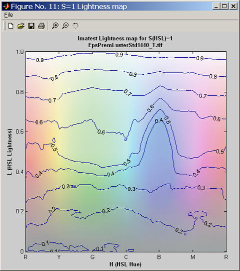
S=1 HSL Hue plot
Colors are labelled 0 to 6, corresponding to hues from 0 to 1. This clarifies the plot by making each primary color an integer: Red = 0 and 6, Yellow = 1, Green = 2, Cyan = 3, Blue = 4, and Magenta = 5. This way, contour increments are 0.5 instead of 0.08667. The ideal Hue map would consist of uniformly spaced vertical lines aligned with the x-axis. The hues here are rather good, but blues are a bit bloated and the magentas are somewhat squeezed. This is also visible on the S=1 Gamut map. There is a highly visible irregularity at L=0.6 on the blue-magenta border (also noticeable on the saturation plot). Hue errors in very light (L>0.95) and dark areas (L<0.1) are not very visible.
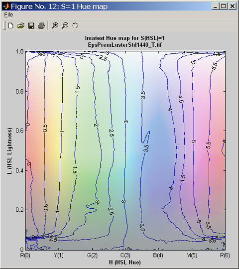
Similar plots are produced for the L=0.5 region, immediately above the S=1 region.
L=0.5 HSL Saturation map
The L=0.5 Saturation map, which displays response to different levels of color saturation, is of interest for comparing different rendering intents (rules that control how colors are mapped when they are transformed between color spaces or color spaces and devices). Colorimetric rendering intents should leave saturation unchanged, at least at low S levels. Perceptual rendering intent expands color gamut when moving to a color space or device with increased gamut; it compresses it when moving to a smaller gamut. But there is no standard for perceptual rendering intent: every manufacturer does it in their own say. "Perceptual rendering intent" is a vague concept; it's hard to know its precise meaning unless you measure it.
The ideal L=0.5 Saturation map would consist of uniformly spaced horizontal lines from 0.9 to 0.1. The weak saturation in the greens and magentas is visible here. From the viewpoint of overall image quality, behavior at low saturation levels is most visible. The Epson 2200 behaves very well in this region.
An additional Figure with L=0.5 HSLHue and Lightness maps has been omitted.
Digitization and Metric Conversion for Image Quality Test Targets by
William Kress discusses the use and accuracy of flatbed scanners for measuring print quality.
Using Test Charts
Creates test charts for high quality inkjet printers
Test Charts
creates test chart files for printing on high quality inkjet printers. Two types of chart can be created: bitmaps and Scalable Vector Graphics (SVG), which can also be sent out for precision printing. A variety of options is available. You can select chart pattern, type (bar or sine), contrast, highlight color, printer gamma, and more.
To run Test Charts, run Imatest and click on Test Charts in the Imatest main window. The following dialog box, which contains the initial (default) settings, appears. The available settings change for different patterns.
The file pixel size and the dimensions when printed at the specified PPI (bitmap files only) is shown on the lower left. The file may be printed at any desired size. Select the Pattern (the type of chart), the options, and the folder (directory) and file name for the test chart file. When you are ready to create the file, click on Create test chart. You may cancel by clicking on Close. When the calculations are complete a figure showing the chart (not for printing) appears. You can zoom in to see the fine detail.
The figure with the image of the chart is for preview only: it shows you what the chart looks like and lets you zoom in if you want. Do not print the chart directly from this figure. Load bitmap Print Test output files (chart_temp.tif in the above example) into an image editor (such as Photoshop, Picture Window Pro, or Irfanview (a great free image viewer that can read and write nearly every known format)) and print it from the editor. SVG (Scalable Vector Graphics) files can be printed from Inkscape (or imported into Adobe Illustrator or Corel Draw). This will allow you to select the size of the print, add annotations, use color management, etc.
The best way to print the charts is to convert the TIFF files from black & white into 24-bit color and print them using a color-managed workflow with ICC profiles. Manufacturer-supplied profiles are usually sufficient; custom profiles may be better when tonal values are critical.
Bitmap patterns
Bitmap patterns consist of arrays of pixels stored as standard image files, in distinction to Vector graphic patterns (below), which consist of scalable primitives such as lines, polygons, etc. Bitmaps are best for continuous-toned images, especially the sine-modulated images described below.
The first three patterns, SFR:quadrants, SFR rectangles, and Distortion grid or checkerboard , are available in all versions. Most of the remaining patterns are available in Imatest Master only.
Print height can be selected in cm (for prints) or pixels (for standard video/screen sizes). Available print sizes are 25x18 cm (for A4 paper), 25x20 cm (for US letter paper), 40x28 cm (for A3 paper), and 40x30 cm (for Super A3/Super B paper). In addition, files can be created with the following sizes, which correspond to standard display resolutions: 640x480, 600x800, 768x1024, 960x1280, 1024x1280, and 1200x1600 pixels.
SFR: quadrants (All versions)
This is the standard chart for SFR measurements. It should be tilted when it is photographed. Instructions are found in Using SFR, Part 1.
Options include adjustment of pixels per inch (100 is recommended), contrast ratio, gamma, and highlight color. |
SFR Quadrants |
SFR: two rectangles (All versions)
This chart is also used for SFR measurements. It should be cut into two segments (left and right sides) and tilted in a manner similar to the SFR quadrants chart, above, when photographed.
Options include adjustment of pixels per inch (100 is recommended), contrast ratio, gamma, and highlight color.
|
SFR Two rectangles |
Distortion grid or checkerboard (All versions)
Distortion grid... generates grid or checkerboard test charts for the Distortion module. (a grid is shown on the right.)
Options include PPI, Highlight color, and Type (Grid or Checkerboard). Maximum contrast is always used. High resolution is not necessary. 100-300 pixels per inch is recommended. |
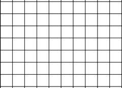
Distortion (grid) |
A portion of the input dialog box for the grid pattern is shown on the right. Several of the popup menu boxes are changed for Grid.
Horizontal divisions and Vertical divisions are specified in the bottom two boxes. 10-20 Horizontal divisions works well in most cases. Vertical divisions has the option, "Square" that makes the grids square. This is the default, recommended in most cases.
Line width (pxls) is typically set somewhere in the range of .01*PPI to .025*PPI. The printed line should be clear (not pale), but not very thick. 3 pixels is appropriate for a 150 PPI file. Lines in the preview image are thicker relative to the grid size than they are in the final image.
The line width should be thick enough to cover at least two pixels in the captured image. Narrower lines may result in errors (Inconsistent number...). For example, suppose your captured image were 640x480 pixels (VGA). The line width (as shown on the right) would be 3 pixels out of a chart width of 1476. In the captured chart, the line width would be 640*(3/1476) = 1.3, inadequate for this small image size, though this chart would be perfectly adequate for 1+ megapixel cameras. |
A portion of the Test Charts input dilog box for
Distortion (showing Checkerboard) |
Star chart (Imatest Master only)
Star charts can be used for observing performance (SFR, Moire patterns, and other image processing artifacts) at a variety of angles. In addition to the star (which has a selectable number of bands and either bar or sine form), the chart contains tonal calibration patches and slanted edges for checking results with SFR.
Standard print sizes are 24x18 cm (for A4 paper), 26.67x20 cm (for US letter paper), 37.33x28 cm (for A3 paper), and 40x30 cm (for Super A3/Super B paper). Options include the number of star bands, sine or bar band pattern (sine shown on the right), pixels per inch (600 or 720 is recommended, depending on the printer), contrast ratio, gamma, and highlight color. Star charts will be analyzed in a future version of Imatest. |
Star chart (original version; not supported by Imatest software) |
|
You can also create the star chart included in the proposed update to the ISO 12233 standard using the following settings: PPI: 720 (Epson inkjets) or 600 (HP or Canon inkjets), Height (cm) (as required), Highlight color: White, Contrast ratio: 40, Type: Sine, Gamma: 2.2, Star pattern bands: 144 or 72, Chart lightness: Lightest, ISO standard chart: Yes or Yes (small inner circle): (inner circle will have 1/10 or 1/20 the diameter of the outer, respectively). This chart can be analyzed with the Star Chart module in Imatest Master.
A high quality printed version of this chart is available from Image Engineering. They describe its use in Measuring the resolution of digital cameras. |

Star chart (proposed ISO std)
Supported by Star Chart
|
Log frequency-contrast gradient charts (or Stepcharts) (1 and 2-band charts in Imatest Master only)
These charts display bar or sine patterns of increasing spatial frequency, for use with two Rescharts modules: Log Frequency and Log F-Contrast. Two options available for creating Step charts. Several features resemble the Koren 2003 test chart described in Lens testing (developed prior to Imatest).
This chart is valuable for viewing Moiré fringing (colored bands caused by aliasing) and analyzing low contrast detail lost as a result of software noise reduction, which takes place inside the camera and/or RAW converter. Software noise reduction is a type of lowpass filtering (reduction of contrast at high spatial frequencies) that is turned on in regions where edges or strong image features are absent. Some may take place even if you try to turn it off. It cannot distinguish noise from high-spatial frequency, low-contrast detail, located in the lower right of the 1 and 2-band charts. The two and four band charts are designed to be cut into segments to be placed around the target, possibly in different orientations (landscape, portrait).
Each chart consists of the following patterns in 1, 2, or 4 bands. From top to bottom,
- A bar pattern of increasing spatial frequency (which could be used to determine spatial frequency (not used in Imatest).
- A sine or bar pattern of increasing spatial frequency (horizontally) for all charts and decreasing contrast (vertically) for 1 and 2-band charts. The contrast is proportional to the square of the distance from the bottom of this band. That emphasizes lower contrast areas, where noise reduction causes a loss of detail. It also corresponds to the way the eye sees, i.e., when the pattern contrast is one quarter of its maximum value, it appears to be about half the maximum. The contrast is constant for the 4-band chart, which is available in Imatest Studio.
 (1-band chart only) 20 rectangular patches. 1 and 20 are black (0,0,0), 2 and 19 are middle gray, and 3-18 (16 patches) are a stepchart with density steps of 0.1. If the chart is printed correctly, i.e., if printer gamma matches the Test Charts setting, these patches will closely match the first 16 patches of reflective step charts with 0.1 density steps such as the Kodak Q-13 and Q-14..
Options include
- Standard options: Pixels per inch (PPI; 600 or 720 is recommended, depending on the printer), Highlight color, Gamma, and Height. The standard print size is 25 x (approximately) 18 cm (9.83 x (approximately) 7.08 inches; A4 paper), 25 x (approximately) 20 cm (9.83 x (approximately) 7.87 inches; US letter paper), 40 x (approximately) 28 cm (15.7 x (approximately) 11.02 inches; A3 paper), 40 x (approximately) 30 cm (15.7 x (approximately) 11.8 inches; Super A3/Super B paper).
- Contrast ratio and Chart lightness: Do not affect patterns with vertically-varying contrast.
- Type: Bar or sine (single pattern), bar or sine (double pattern), or bar and sine without contrast variation (quad pattern; available in Imatest Studio).
- Frequency ratio (maximum to minimum) See Log F-Contrast for recommendations.
- Maximum spatial frequency in cycles/width. (The actual spatial frequency will be detected by the analysis program.) See Log F-Contrast for recommendations.
The two Stepchart options include a chart with 20 steps (similar to the Kodak Q-13) and with16 steps with black and middle gray bands at the ends. Both have a density increment of 0.1. They can be printed any size (small or large) and sliced into narrow strips for specialized testing. Stepcharts should be printed with care in a color-managed environment. If an ICC profile is used for printing, Black Point Compensation should be turned off. For most applications, standard charts such as the Kodak Q-13 and Q-14 are recommended for best accuracy.
Zone plate (Imatest Master only)
Zone plates (based on Fresnel diffraction) are useful for observing aliasing, particularly Moire patterns and other image processing artifacts. They have a much larger area of high spatial frequencies than the star chart. The spatial frequency is inversely proportional to the square of the radius (the distance from the center of the pattern). The chart also contains tonal calibration patches and slanted edges for checking results with SFR. Thanks to Bart van der Wolf, who has done some interesting work with zone plates.
|
Zone plate |
Print sizes are the same as the star chart. Options include a divisor for the maximum spatial frequency (0.5 cycles per pixel at the outer radius when set to 1), sine or bar band pattern (sine shown on the right), pixels per inch, contrast ratio, gamma, and highlight color. Low ppi charts are useful for testing resizing performance.
Scalable Vector Graphics (SVG) patterns
Vector graphic images consist of primitives such as lines, polygons, etc., that can be scaled to any size and do not suffer from the pixellation problems of bitmap images. They print at the printer's maximum quality, regardless of size. Vector graphics are excellent for generating test charts consisting of lines, curves, and areas that don't require complex tone variations such as sine modulation.
Scalable Vector Graphics (SVG) is an XML file format recognized by the World Wide Web Consortium (W3C). SVG files can be read, edited, and printed by Inkscape— an excellent free open-source program (described in Wikipedia). They can also be imported into Adobe Illustrator, Corel Draw, and others. SVG implementations are listed here.
Imatest Master can create two types of SVG chart, discussed in detail in SVG (Structured Vector Graphics) Test Charts.
SVG Squares & Wedges (letter, A4, ...)
This was the first SVG pattern to be included in Imatest. It consists of tilted squares, "hyperbolic" wedges, bars of varying spatial frequencies, and a replica of the Kodak Q-13 step chart with density steps of 0.1. It is optimized to be printed A4 or letter size on a high quality inkjet printer and mounted on a 3x3 grid, as shown on the right— though it can be printed any size without loss of quality. In this arrangement it will have a field width of around 32 inches (80 cm), sufficient for measuring the performance of the best modern DSLRs.
The chart below was created using Contrast ratio = 20, Gamma = 2.2, Highlight color = White, and Chart lightness = Light. Additional details are found on SVG (Structured Vector Graphics) Test Charts.
|
3x3 chart arrangement (for letter/A4 prints) |
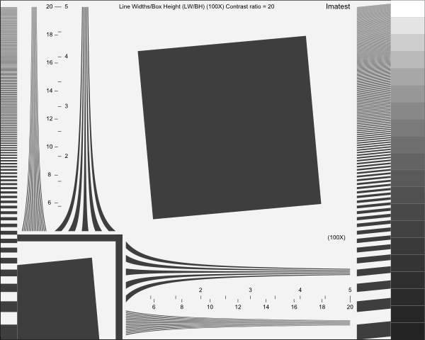
Slanted squares on m x n grids
The rest of the SVG charts consist of slanted squares arranged on an m x n grid. A step chart (density increment = 0.1) and a pair of hyperbolic wedges may be optionally added. The chart's contrast, brightness, and several other details are adjustable. A typical SVG SFR chart, consisting of a 5x9 grid, is shown below.
SVG SFR chart: 5x9 grid, 20:1 contrast, with optional hyperbolic wedge
and step patterns (0.1 density increment) .
This chart is optimized to print at 20x36 inches (50x90 cm) or larger. It should not be printed small (letter-size or A4) on inkjet printers because SFR test results would be limited by the printer's resolution. Other grid patterns are available that are optimized for printing at different sizes. Grid choices include 1x2, 2x3, 3x5, 4x7, 5x9, and 7x11. The larger grids (3x5 and up) are optimized for printing on wide format printers, and are available in Imatest Master only. Additional details, as well as instructions on how to print these charts, are found on SVG (Structured Vector Graphics) Test Charts.
Options
Pixels per inch (PPI)
(bitmap charts only) Choices: 720,
600,
400,
360,
320,
300,
180,
150,
120,
100,
72
Along with chart height, PPI determines the size of bitmap test chart image files. For the two SFR charts (1 and 2 above) it can be a low number— 100 PPI, because there are only vertical and horizontal edges. For the Star, Log frequency, and Zone plate charts, the native DPI (dots per inch) of the printer is recommended: 720 for Epson printers (1440 or 2880 dpi); 600 for Canon or HP (1200, 2400, etc. DPI). High resolution files can be somewhat slow to create.
Chart height
(bitmap charts only) Choices: 30 (Super A3/B),
28 (A3),
20 (US Letter),
18 (A4)
The intended height of printed bitmap charts, assuming landscape format (where width > height). The chart can be printed any size, but when it is printed at the intended height, the the specified PPI (above) is sent to the printer. This gives optimum results. The width is larger than the height by a roughly 4:3 ratio (depending on the pattern). The specified heights are 18 cm (7.08 inches; A4 paper), 20 cm (7.87 inches; 11x8.5 inch US letter paper), 28 cm (11.02 inches; A3 paper), and 30 cm (11.8 inches; 19x13 inch Super A3/Super B paper).
Highlight color
In addition to the standard White/Black (or White/Gray) charts, you can replace white with any additive or subtractive primary color: R, G, B, C, M, or Y.
Different colors are of particular interest in analyzing Bayer sensors, where alternate rows of pixels are sensitive to {R, G, R, B, R, ...} and {G, B, G, B, G, ...}. Since there are only half as many R and B sensors as green sensors (and one quarter as many as total pixels), one would expect MTF to be poorer for red-black and blue-black charts than for white-black). Demosaicing algorithms typically make use of different colored pixels for calculating detail (i.e., an edge in the red channel would be sharper if information is present in the other channels). Also, different algorithms perform differently. A lot can be learned from targets of different colors.
Chart lightness
Choices: Lightest,
Light,
Mid-light,
Middle,
Mid-dark,
Darkest
Determines the grayscale level of both the light and dark areas of the chart. Useful with charts that contain grayscale information (star, zone plate, and Log frequency patterns with sine modulation), where best pattern quality can be obtained if this setting is not "lightest" (highlights pure white). Also valuable for SFR edge charts, where middle tones are likely to be in the camera's linear response region.
Type (bar or sine)
(bitmap charts only) The features of the star, zone plate, and Log frequency patterns can be either bars (shown in the Magenta star pattern, above), or sine (shown in the White-Black Star, Log frequency-contrast, and Zone plate patterns, above). Sine patterns are not available in SVG charts.
Star pattern bands
The number of bands in a star pattern is selectable. It is always a multiple of four. The nearby Magenta pattern has 36 bands (the default); the White-Black pattern shown above has 20 bands. Commercially-available star patterns come in a wide variety.
Contrast ratio
Choices: None, Maximum, 80, 50, 40, 25, 20, 10, 5, 4, 2, 1.414, 1.2, 1.1
The ratio of the reflectivity of the light to dark areas (the upper zone only in the Log frequency chart). The maximum contrast ratio depends on the printer and paper. It is typically around 100 for glossy (or luster) surfaces, but only around 40 for matte surfaces. Maximum print density = -log10(minimum reflectivity) can be measured in Print Test or estimated by Gamutvision. Available selections are Maximum and 80 through 1.1.
Clipping is often a problem with high contrast targets. The ISO-12233 standard calls for a contrast ratio between 40 and 80, but recent experiments have shown that lower contrast ratios produce more accurate and consistent results, which are less affected by gamma and camera nonlinearities. In 2007 the ISO standard will change to recommend lower contrast chart. The default value for Test Chart is 40 (the minimum recommended in the ISO standard), but 20 is preferred in many cases.
Contrast ratio affects MTF (SFR) measurements in cameras that perform nonlinear signal processing, i.e., noise reduction and sharpening with thresholds— nearly universal in consumer cameras. Charts with at least two contrast ratios: 20 and 2 (or lower) are recommended for characterizing cameras.
Gamma
Choices: 2.5, 2.2, 2.0, 1.8, 1.5, 1.0
You should use the value of gamma for your typical color space and workflow (2.2 is standard for Windows; 1.8 for older Mac systems). The default value is 2.2. Gamma affects the accuracy of sine patterns and the actual printed contrast ratio: it must be the same value used for printing (the value of the color space, i.e., 2.2 for Adobe RGB (1998), if color management is used) to get the correct contrast ratio.
Ink spread compensation
corrects for ink spread (or "dot gain") in the Log frequency chart. (The Star chart may be added later.) The best value has to be determined experimentally.
Output figure
The output figure contains an image of the test chart. It is not anti-aliased, hence lines may be missing (in Grid) or curious aliasing patterns may appear, visible below. Only the circle in the middle is real-- all the others are the result of aliasing.
This figure is not intended for printing. To print a chart open the image file (C:\Imatest\Data_distortion\chart_temp.tif in the example below) in an Image editor and print it from the editor. A high quality (photographic) inkjet printer is recommended. The best way to print the charts is to convert the TIFF files from black & white into 24-bit color and print them using a color-managed workflow with ICC profiles. Manufacturer-supplied profiles are usually sufficient; custom profiles may be better when tonal values are critical.
Preview image of Zone plate showing extreme Moiré
You can zoom in on the chart by selecting an area or clicking on a point of interest. Double-clicking restores the complete image.
Preview image of Zone plate, zoomed in
Using Screen Patterns
Monitor patterns for Light Falloff, SFR, Distortion, and monitor calibration
Introduction
Screen Patterns displays a variety of test patterns on monitors, preferably on LCD flat screen monitors. It is opened by clicking on Screen Patterns on the right of the Imatest main window. Most patterns (except perhaps Monitor calibration) perform best with the window maximized. You may need to redraw the pattern after maximizing (or resizing) it by selecting the pattern or changing one of the settings. These patterns are offered as a convenient alternative to the printed patterns created by Test Charts, and in one case— Light Falloff— the use of Screen Patterns is superior to other techniques.
The test patterns fall into two categories:
- patterns that can be photographed for analysis by Imatest modules, including Light Falloff, Distortion, and SFR, and
- patterns for checking monitor calibration, estimating monitor performance (and a few other uses).
The pattern is selected with a dropdown menu in the bottom-middle of the Screen Patterns window. The patterns intended for photographing tend to work poorly with CRTs because of the raster scan, which can cause nonuniform illumination and may cause inconsistent readings with some DSLR metering systems (like my Canon EOS-40D). The patterns are summarized in the table below.
| Patterns to be photographed for Imatest analysis (not recommended with CRTs) |
| Light Falloff (blank) |
Blank screen for obtaining even illumination. Superior to other low-cost techniques. |
| SFR Quadrants |
SFR quadrant pattern: you must tilt the screen relative to the camera to photograph it. |
| SFR Quads: Global H,S |
SFR quadrant pattern where darker (quadrant) areas have the same H and S as the highlight area (normally the darker area is neutral). |
Distortion grid
Distortion grid inverted |
A large LCD flat screen monitor is a definite asset with this module. |
Slanted edges
(1, 2, and 3 rows) |
Similar to the patterns in SFR SVG Test charts. 1, 2, and 3 row patterns are available. Not as sharp as the SFR quadrant patterns (with vertical, horizontal edges). Use with care; not for testing high resolution cameras. |
| Miscellaneous: for monitor calibration or camera adjustment |
| Monitor calibration |
This selection contains several patterns:
A gamma/black level test pattern that allows you to estimate gamma,
A monitor gamma pattern that looks uniform when the adjacent slider is set to the correct gamma, and
Two HSL rainbow patterns that can be used for a rough visual estimate of color quality. |
| Monitor gamma only |
The monitor gamma pattern fills the entire screen. It is adjusted with a slider at the bottom-center. It allows you to determine gamma with high accuracy and see variations across the screen. |
Zone plate (sine)
Zone plate (bar)
|
For finding optimum camera focus using strongly visible moiré patterns. Sine and Bar options are available. |
| SMPTE color bars |
Widely used for video adjustments. May be used for a simple visual analysis of color quality. |
| Colorchecker and Stepcharts |
Simulated Colorchecker and Stepcharts: 20 steps with 0.10 and 0.15 density steps (1.95 and 3.85 maximum densities). NOT for camera testing. |
Some of these patterns have no well defined uses, but we include them because customers often find uses we cannot anticipate. Adding charts to Screen Patterns is relatively straightforward. Please contact us if you'd like to have one added.
Several patterns display the W x H screen size in the lower right corner. H is smaller than the total screen size by about 21 pixels: about the hight of the upper toolbar.
Light Falloff pattern
If you have a flat screen LCD monitor, the Screen Patterns Light Falloff pattern is the best way of obtaining an even, uniform image. This is the first pattern that appears when you open Screen Patterns.
Light Falloff image (initial screen at startup)
Maximize this pattern for best results. Hue, Saturation, and Lightness (H, S, and L, which default to 0,0,1) can be adjusted using the sliders on the far left. HSL and RGB values are displayed at the bottom. Photograph it at a distance of 1-3 inches (2-8 cm). (Thanks to Jonathan Sachs for this suggestion.)
For extreme wide angle lenses or laptop screens with a limited viewing angle, an additional diffuser should be used. We recommend using opal diffusing glass mounted close to the lens. Opal glass is available in the US from Edmund Optics. (Thanks to Bart van der Wolf for the suggestion.) If a diffuser is used, a lightbox may be substituted for the monitor. (Lightboxes are typically brighter but less uniform.)
SFR patterns
There are two quadrant patterns for SFR measurements:
- SFR Quadrants,where the darker area is neutral, and
- SFR Quads: Global H,S, where the darker area has the same Hue (H) and Saturation (S) as the highlight area.
The monitor should be tilted (typically around 5 degrees) with respect to the camera when this pattern is used for SFR measurements. (The pattern itself is not tilted because this would result in pixellation.) This use of this pattern is discussed in Imatest SFR LCD target. |
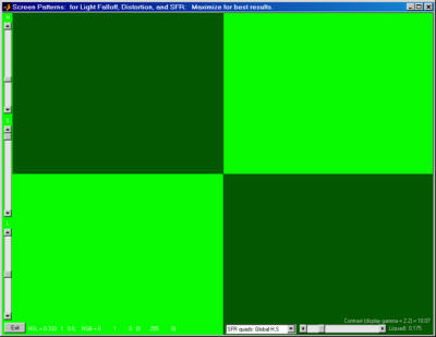
SFR pattern (Global H,S): Shown in pure green with
10:1 contrast. (Default is White and Black.) |
Highlight H, S, and L can be controlled with the sliders on the far left. Quadrant Lightness (L) can be controlled with the slider on the bottom-right. The contrast for display gamma = 2.2 is shown on the lower right. In this case (pure green; not the default), the lower right slider has been adjusted for a 10:1 image contrast. The L slider on the left is set to 0.5 for maximum color saturation.
Distortion grid
The distortion grid creates images for the Imatest Distortion module consisting of black lines on a white or colored background. It works best with the window maximized. (The image may need to be redrawn after resizing.) It should not be used with CRTs, which are notoriously subject to distortion, except to measure the distortion of the CRT itself using a lens of known low distortion.
Three key settings are located on the lower-right: the number horizontal lines (H-L), the number of vertical lines (V-L), and the line width in pixels (W). The choice depends on the amount of distortion and the aspect ratio of the screen. The first (default) vertical setting is Square: vertical and horizontal lines have identical spacing. 7-9 horizontal lines and 10-15 vertical lines are typical. The Squares pattern (below) can also be used with Distortion, and may well be more robust than the grid.
|
Distortion grid |
Normally the lines are black and highlight (background) H, S, and L can be controlled with the sliders on the far left. If Distortion grid inverted is selected, the background will be black and the H, S, and L sliders will adjust the line color. |
Distortion grid inverted |
Monitor calibration
This selection contains several patterns that enable you to check your monitor's calibration. The gamma patterns (left and middle) must be viewed on a monitor; they do not work in printed media. Reset pattern restores the default values, H = 0, S = 0, L = 1, and Gamma = 2.2.
Note that laptop LCD screens cannot be accurately calibrated because gamma is a strong function of vertical viewing angle.
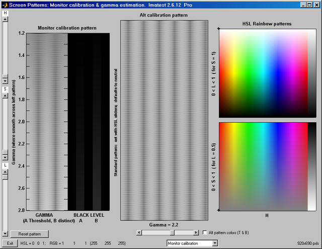
Monitor Calibration patterns (the serrated vertical bands
in the left and middle patterns are not what you see.)
Left: Gamma and black level chart adapted from normankoren.com.
This chart enables (shown below) you to set the black level (brightness) and estimate display gamma over a range of 1.2 to 2.8 with accuracy close to ±0.05. The gamma pattern is on the left; the black level pattern is on the right. Before using the chart, CRT monitors should be turned for on for at least 15 minutes. For flat screen (LCD) monitors, Screen resolution should be set to the monitor's native resolution (right-click on the wallpaper, Properties, Settings).
Display gamma is the relation between pixel level and screen luminance. It comes from the equation,
Luminance = (pixel level)gamma |
Gamma is estimated by locating the position where the average luminance across the gamma pattern is constant. The corresponding gamma is shown on the left. You should be far enough from your monitor so the line pattern is not clearly visible. The example below shows what to look for.
This chart features gradual density changes along horizontal scan lines (thus eliminating CRT risetime problems).
What to look for
(for Gamma = 2.0)
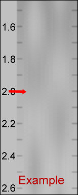
|
|
Your monitor's gamma should be set for 2.2 (for Windows systems).
Gamma = 2.2 for the Internet-standard sRGB color space and the popular Adobe RGB (1998) color space. 1.8 was the standard for older Macintosh systems and prepress file interchange (Mac users, see Ian Lyons' Mac Calibration page.).
Most laptop LCD screens cannot be accurately calibrated because gamma is extremely sensitive to viewing angle.
You can adjust gamma using Quickgamma (a great free program) or a hardware calibrator (details here). |
We'll be happy to grant permission to reproduce this pattern on your website if you e-mail us, give credit and a link to this page. |
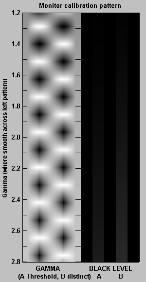
|
Black level (brightness) Your monitor's brightness control (which should actually be called black level) can be adjusted using the mostly black pattern on the right side of the chart. This pattern contains two dark gray vertical bars, A and B, which increase in luminance with increasing gamma. (If you can't see them, your black level is way low.) The left bar (A) should be just above the threshold of visibility opposite your chosen gamma (2.2 or 1.8)-- it should be invisible where gamma is lower by about 0.3. The right bar (B) should be distinctly visible: brighter than (A), but still very dark.
There is considerable interaction between the brightness and gamma settings in CRTs— increasing brightness decreases gamma-- so you may have to go back and forth two or three times. There is less interaction between Contrast and gamma. The vertical bars correspond to normalized luminances of 0.002 and 0.006 at the specified gamma.
|
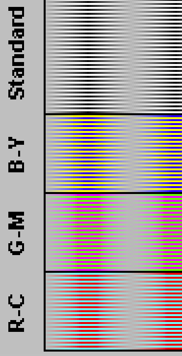
Alt calibration pattern (middle) enlarged 4x;
Alt pattern colors (T & B) checked |
The image on the right shows the middle gamma pattern enlarged 4x. The upper part of this image, to the right of Standard, uses the same black-to-white sinusoidal variation as the Gamma and black level chart. The color patterns appear when the Alt pattern colors (T & B) box, located just to the right of the Gamma slider, is checked
When this image is displayed normal size (not enlarged; below) on a good quality monitor, the R-C, G-M, B-Y, and Standard patterns appear nearly identical. |
Middle: Gamma pattern. This pattern will look uniform when the gamma slider (just below it) is set to the correct monitor gamma. It is very sensitive: it can measure gamma to better than ±0.05 accuracy: The spatial frequency of vertical bands is set close to the the frequency where the human eye's Contrast Sensitivity Function is maximum for typical viewing situations.
The patterns on the right will appear uniform
if monitor gamma is 2.2.
A checkbox labeled Alt pattern colors (T & B) is located just to the right of the Gamma slider. When this box is checked, three bands (six total) appear near the top and bottom of the gamma pattern. Instead of the standard gamma pattern's normal black-to-white sinusoidal variation, individual lines vary from Blue-to-Yellow, Green-to-Magenta, and Red-to-Cyan. In a normally functioning monitor these bands appear the same neutral gray as the standard pattern, but they could look strange in a defective or poorly calibrated monitor. Unchecking this box speeds image refresh. |
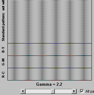
Middle (gamma) pattern,
showing R-C, G-M, B-Y color bands |
Right: HSL rainbow patterns. These patterns are used for a rough visual estimate of the monitor's color performance. They should appear well-saturated and have smooth color and tonal gradations (no abrupt changes). Laptops typically look very different from well-calibrated LCD or CRT monitors.
Gamma pattern (full screen)
The full screen gamma pattern allows you to examine screen uniformity in fine detail. It is identical to the gamma pattern in the middle of the Monitor calibration display, described above. Gamma can be estimated with excellent accuracy: to better than ±0.5.Hightlight H, S, and L can be controlled with the sliders on the far left. Reset pattern restores default values: H = 0, S = 0, L = 1, and Gamma = 2.2. |
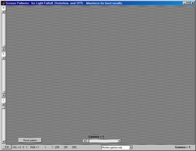
Full screen gamma pattern
for viewing screen
nonuniformities. (Actual image looks very different) |
Zone plate
The zone plate is useful for testing camera focus in cameras with live view because it produces highly visible moiré patterns when it is photographed or resized; the stronger the moiré the better the focus. It works best with the window maximized (it may need to be redrawn after resizing.) Northlight Images describes a way of using the zone plate to tune the focus of the Canon 1Ds Mark III. The Squares patterns below are also designed to generate moiré.
Screen Patterns has two versions of the zone plate: sine (shown below) and bar (with stronger edges: possibly better for focusing).
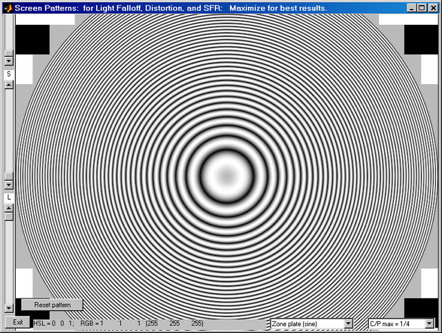
Zone plate pattern
The maximum spatial frequency can be adjusted with the menu on the bottom right. 1/4 cycles/pixel (half-Nyquist) is the default. Highlight H, S, and L can be controlled with the sliders on the far left. (The H slider was obscured when the image was resized.) Reset pattern restores default values: H = 0, S = 0, L = 1 and also redraws the image. Learn more about zone plates from Bart van der Wolf.
SMPTE color bars
SMPTE color bars are widely used in the video industry for calibrating TVs and monitors. They're included in Screen Patterns as an experiment— to see if customers find them useful. It's straightforward to add charts to Screen Patterns: please contact us if you have a chart you'd like added.
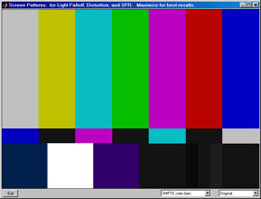
SMPTE color bar (original) |
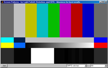 SMPTE color bar (HD)
 |
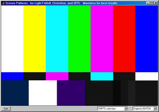
SMPTE color bar (original LIGHTENED): upper section lightened |
The pixel values for the charts are from the Wikipedia page, SMPTE color bars. We are not certain of their correctness. Many pages interpret these bars differently (the colors in the top row are often brighter). Both the original and HD charts can be displayed with the top row of colors lightened.
Slanted edges (1, 2, and 3 rows)
These slanted edge patterns are similar to the patterns in SFR SVG Test charts. 1, 2, and 3 row patterns are available. H, S, and L (Hue Saturation, and Lightness) can be adjusted for the highlights (i.e., the background), and L can be adjusted for the patches, which retain the same H and S values as the background, similar to SFR Quads: Global H,S , described in SFR quadrant patterns, above. Contrast is displayed on the lower right.
It is important to note that these edges are not as sharp as the vertical and horizontal edges in SFR quadrant patterns because a small amount of anti-aliasing must be applied to avoid jagged edges. These patterns are not generally recommended for testing high resolution cameras, where large printed charts work far better, but they may be useful in testing monitors, projectors, and low resolution cameras. If all cases, you should carefully analyze the relative contributions of the display, camera, and lens to the final MTF measurement, i.e., you should know precisely what you are measuring.
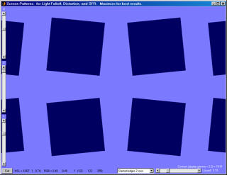
2-row slanted-edge pattern, 20:1 contrast |
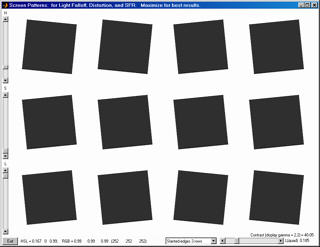
3-row slanted-edge pattern, 40:1 contrast |
Colorchecker and Stepcharts
A simulated GretagMacbeth ColorChecker and two step charts are displayed. sRGB color space (gamma = 2.2) is assumed. The upper stepchart has a density increment of 0.10 and range of 1.9 (79:1 contrast ratio); the lower stepchart has a density increment of 0.15 and range of 2.85 (708:1 contrast ratio).
This pattern should never be used for testing cameras: a real reflective Colorchecker should always be used. It can be used to make a simple visual estimate of display quality, and it may also be useful for analyzing the response of displays or projected images when photographed with a well-profiled camera. |
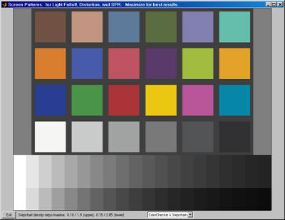
Colorchecker & Stepcharts (ΔD = 0.10, 0.15) |
Squares (Checkerboard) and Squares with focus pattern
These patterns are specifically designed for creating moiré fringing for measuring camera focus with a camera's Live View feature. See Bart van der Wolf's post on Open Photography Forums and related material on Northlight Images. The Squares (checkerboard) pattern (left, below) is an alternative to the grid chart in Distortion.
Squares (checkerboard) |
Squares with focusing pattern |
The spacing between squares (1-30) or the number of squares (for Squares (checkerboard) only) can be selected in the window in the lower right.
SVG (Structured Vector Graphics) Test Charts
for improved MTF measurements
Test Charts
creates test chart files for printing on high quality inkjet printers. This page focuses on Scalable Vector Graphics (SVG) charts for measuring sharpness (MTF) with Imatest SFR and SFRplus. (Bitmap charts are described elsewhere.) SVG charts can be printed any size at a printer's maximum quality (i.e., resolution) with no limitations, and they generally require much less storage than bitmap images. Several of the SVG charts are well suited for automated testing with SFRplus and have numerous advantages over the widely-used ISO 12233 chart.
Vector graphic images consist of primitives such as lines, polygons, etc., that can be scaled to any size and do not suffer from the pixellation problems of bitmap images. They print at the printer's maximum quality, regardless of size. Vector graphics are excellent for generating test charts consisting of lines, curves, and areas that don't require complex tone variations such as sine modulation.
Scalable Vector Graphics (SVG) is an XML file format recognized by the World Wide Web Consortium (W3C). SVG files can be read, edited, and printed by Inkscape— an excellent free open-source program (described in Wikipedia). They can also be imported into Adobe Illustrator, Corel Draw, and others. SVG implementations are listed here.
Imatest can create SVG files consisting of lines and polygons, but unfortunately not circles or Bezier curves. This is sufficient for making outstanding targets for measuring SFR and aliasing (moiré patterns, usually colored). Contrast, lightness, and highlight color are selectable.
Introduction: SVG chart designs and advantages
Slanted squares on m x n grids
Most of the SVG charts consist of slanted squares arranged on an m x n grid. A step chart (density increment = 0.1) and a pair of hyperbolic wedges may be optionally added to some of the charts. The chart's contrast, brightness, and several other details are adjustable. The standard SVG chart for SFRplus, consisting of a 5x9 grid, a 4x5 stepchart, and bars at the top and bottom, is shown below.
SVG SFR chart: 5x9 grid, 10:1 and 2:1 contrasts, with optional step pattern
(0.1 density increment).
Designed for the new automated SFRplus module.
This chart is optimized to print at 20x36 inches (50x90 cm) or larger and is designed to work with the new SFRplus module that has automatic ROI (Region of Interest) selection. In addition to MTF, it is useful for measuring lateral chromatic aberration, lens distortion, gamma (contrast), and tonal response. It should not be printed small (letter-size or A4) on inkjet printers because SFR test results may be limited by the printer's resolution. Other grid patterns are available that are optimized for printing at different sizes. Grid choices include 1x2, 2x3, 3x5, 4x7, 5x7, 5x9, and 7x11. The smaller grids (1x2 and 2x3) are designed to be printed relatively small (up to 13x19 inches) with several mounted on large foam boards (32x40 inches or larger). The larger grids (3x5 and up) are optimized for printing on wide format printers, and are available in Imatest Master only.
The squares are tilted as shown to facilitate the measurement of Lateral Chromatic Aberration, which is done best using tangential (or near-tangential) edges near the boundaries of the image.
SVG charts have a number of significant advantages over the standard ISO 12233 chart, shown on the right. |
 ISO 12233 chart
. |
- Far less wasted area. The ISO chart was designed by committee. (I know some members who joke about it.) Less that 10% of its total area is useful for SFR measurements; 90% is wasted. Slanted-edges may not be available in important regions, such as the corners.
- Larger ROI location tolerance. Imatest SFR requires that ROIs (regions of interest) be selected prior to the run. On the ISO chart, very limited areas are usable for ROIs. If the ROI selection is made carelessly, interfering patterns may spoil the measurement. The relatively large squares in the SVG charts allow for considerable tolerance. The illustration below shows how the ROI can be shifted much further (vertically) for the SVG chart. The square in the ISO chart is very small: the ROI needs to be as large as possible to ensure good results.
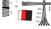
ISO chart ROI selection:
Low (vertical) position tolerance. |
SVG chart ROI selection:
High position tolerance. |
- Better suited to automated testing. The spacing of the slanted squares, the absence of interfering patterns, and the large ROI selection tolerance in the SVG charts is highly compatible with automated ROI refinement, available with Imatest Master 2.6 (released January 2008). This feature allows regions to be automatically refined (shifted) in repeated runs, where it may not be possible to maintain exact chart alignment.
- Better contrast control: less clipping. The standard ISO chart is specified to have a minimum contrast ratio of 40:1, and is typically printed closer to 80:1. This often results in clipping in the shadows or highlights (image too close to levels 0 or 255; sometimes both) in contrasty digital cameras . It can also reduce the accuracy of MTF measurements because many cameras have complex tonal response curves (pictorially-pleasing "S" curves), which are hard to linearize. This problem has been recognized by the ISO committee, which is designing charts with much lower contrast for the revised standard (which will include several charts rather than trying to fit all measurements into one chart). A 10:1 contrast ratio is a good choice for a (relatively) high-contrast chart.
| "Previous target designs had several resolution features that, while visually and instinctively appealing, offered little to enable automated and robust camera evaluation. The predominance of high contrast features, lack of in situ neutral gray patches, absence of machine-vision registration features, and unnecessary complexity are, in retrospect, seen as design flaws." |
|
- Lateral Chromatic Aberration (LCA). The vertical edges near the left and right borders are oriented tangentially to facilitate LCA measurement.
- Nonlinear image processing. Many (perhaps most) digital cameras employ some type of nonlinear signal processing to enhance image appearance. In practice this means that sharpness is increased (MTF is boosted at high spatial frequencies) in the proximity of contrasty edges and noise is reduced (MTF is cut at high spatial frequencies) if there are no contrasty edges nearby. Hence, low and high contrast edges often have very difference MTF response. The SVG charts can have two contrasts (primary and secondary), as illustrated below: primary contrast is 20:1; secondary contrast (in two sections) is 2:1. Tones have been inverted to illustrate one of the many options.
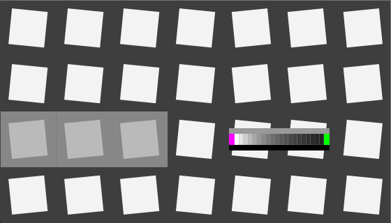
SVG SFR chart: 4 x7 grid, inverted tones, 20:1 primary (2:1 secondary) contrast,
with optional step pattern (0.1 density increment).
Imatest can supply custom SVG test charts in a variety of sizes. Contact
for details.
SVG Squares & Wedges (for printing letter size, A4, etc.)
This pattern consists of tilted squares, "hyperbolic" wedges, bars of varying spatial frequencies, and a replica of the Kodak Q-13 step chart with density steps of 0.1. It is optimized for printing A4 or letter size on a high quality inkjet printer and mounted on a 3x3 grid, as shown on the right— though it can be printed any size without loss of quality. This arrangement it will have a field width of around 32 inches (80 cm), sufficient for measuring the performance of the best modern DSLRs.
If you require a chart printed on a single sheet or if you plan to do automated testing, one of the m x n slanted square on grid charts described above (preferably 5x9) is recommended. |
3x3 chart arrangement (for letter/A4 prints) |
The chart below was created using Contrast ratio = 20, Gamma = 2.2, Highlight color = White, and Chart lightness = Light. The highlight and dark pixel values are 243 and 62, respectively, resulting in a display contrast of (243/62)2.2 = 20.2 at display gamma = 2.2. One or two of the corner charts could have very low contrast (2 or lower) to better characterize cameras with nonlinear signal processing.
A contrast ratio of 20 is high enough to turn on the maximum sharpening in cameras with nonlinear signal processing (which sharpen only in the presence of edges), but not so high that it is likely to cause clipping (pixel levels 0 or 255). It is half the minimum value of 40 in the soon-to-be-replaced ISO 12233 standard, now understood to be too high for reliable results. We also recommend printing a low contrast target— with contrast = 2 or lower— to better characterize camera performance. Results at contrasts = 20 and 2 will differ— often strongly— in the presence of nonlinear signal processing, which is nearly universal in consumer digital cameras.
SVG Squares and Wedges pattern
Chart details: The edges in the center square and the solid on the lower right are tilted approximately 5.7 degrees (arctan(0.1) ) for use in SFR. The converging line patterns ("hyperbolic" wedges) are intended for viewing moiré patterns: colors resulting from aliasing near the Nyquist frequency. They will eventually be analyzed in a module that includes the CIPA DC-003 measurements . The high frequency pattern goes from 400 to 2000 line widths/box height (LW/BH), where "box height" is the distance from the top to bottom of the active chart area (the rectangle just inside the outer rectangle, which represents the entire page). The low frequency pattern goes from 50 to 500 LW/BH. To convert to line widths per picture height (LW/PH), multiply LW/BH by the vertical pixel count and divide by the number of vertical pixels in the box. Some scale marks are omitted because of chart crowding.
The bar patterns on the left and right vary in spatial frequency from about 50 to 2000 LW/BH. They are uncalibrated. The step chart pattern on the right has density steps of 0.1 if the image is printed correctly: it is a replica of the Kodak Q-13 chart. If the printout is correctly calibrated, i.e., if the printer actually prints with the specified gamma, a Kodak Q-13 chart placed adjacent to the pattern will have identical tones (by visual inspection or scanner image readout). In this case, the printed chart contrast (10 in the above example) will be as specified.
Two charts are available for download. Each is 304 KB (SVG) or 500 KB (PDF— for those of you who don't want to bother installing Inkscape). Right-click on the links to save the file.
- Contrast = 20, light, gamma = 2.2, white highlights (SVG) | Contrast = 20 (PDF) High enough contrast to excite maximum sharpening in most cameras but low enough to avoid clipping in most cases.
- Contrast = 2, middle, gamma = 2.2, white highlights (SVG) | Contrast = 2 (PDF) Relatively low contrast: little, if any, sharpening would be expected. The two charts should have the same MTF if little or no nonlinear processing is applied, for example, with RAW files with dcraw conversion.
The high contrast (20:1) chart may be too contrasty for some cameras— highlights and/or shadows may clip. Chart contrast can be edited by opening the chart in Inkscape and selecting the white area of the image. A message at the bottom of the window will say something like, "Group of 5 objects in root." Rght-click, select Ungroup, click outside the object, then click inside the white area again. Now the message at the bottom will say something like, "Group of 548 objects in root." Again, right-click, select Ungroup, click outside the object, then click inside the white area. This time the message at the bottom should say, "Group of 1 object." Click on Object, Fill and Stroke... Select the Fill tab and click on the Flat color box (to the right of X). Click on the HSL tab. The original value of L should be 243 for this chart (it may not display). Set L for a a lower value. Around 200-220 should work well, even for very contrasty cameras. The final contrast for charts printed at gamma = 2 2 is (L/62)2.2.
Operation
To run Test Charts, run Imatest and click on Test Charts in the Imatest main window. The following dialog box, shown for a 5x9 SVG grid pattern, appears. The available settings change for different patterns. Pattern selections for the SVG charts are shown in boldface on the left.
Test Charts input dialog box for SVG patterns
Pattern selections
SFR: quadrants
SFR: 2 rectangles
Grid
Star
Log frequency-contrast
Zone plate
|
SVG Squares & Wedges (letter, A4...)
SVG Squares 1x2 (letter, A4...)
SVG Squares 2x3 (>=A3)
SVG Squares 3x5 (>=Super A3/B)
SVG Squares 4x7 (>=Super A3/B)
SVG Squares 5x7 (>= 50 cm (20") h)
SVG Squares 5x9 (>= 50 cm (20") h)
SVG Squares 7x11 (>= 60 cm (24") h)
SVG Squares 2x3 (Same orientation) |
Select the Pattern (the type of chart), the options, and the folder (directory) and file name for the test chart file. When you are ready to create the file, click on Create test chart. You may cancel by clicking on Close. When the calculations are complete a figure showing the chart (not for printing) appears. You can zoom in to see the fine detail.
The figure with the image of the chart is for preview only: it shows you what the chart looks like and lets you zoom in if you want. Do not print the chart directly from this figure. To print SVG charts, load the Print Test SVG output file (chart_temp.svg in the above example) into an editor that supports SVG. (Inkscape is recommended; Adobe Illustrator, Corel Draw, and others can also be used.) This will allow you to select the size of the print, add annotations, use color management, etc.
Options
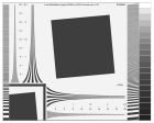 Pattern
Two types of SVG pattern are available: Squares and Wedges (shown on the right; described above), and squares on a grid (1x2, 2x3, 3x5, 4x7, 5x9, or 7x11; described above). The Squares and Wedges pattern and the 1x2 patterns are designed to be printed small (letter-sized or A4) and mounted in a grid arrangement (typically 3x3) to be photographed. The other grid patterns (3x5 and larger) are designed to be printed larger. The 5x9 and 7 x11 charts are particularly well suited for large format (24 inch and greater) printing. The 2x3 (same orientation) chart is designed to be printed up to Super A3/B (13x19 inches) and placed near the corners of a large target (typically 40x60 inches; 1x1.5 meters). This requires that two of the charts be printed as mirror images, which can be obtained in Inkscape by selecting the chart then clicking on Object, Flip Horizontal.
Highlight color
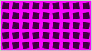 In addition to the standard White/Black (or White/Gray) charts, you can replace white with any additive or subtractive primary color: R, G, B, C, M, or Y.
Different colors are of particular interest in analyzing Bayer sensors, where alternate rows of pixels are sensitive to {R, G, R, B, R, ...} and {G, B, G, B, G, ...}. Since there are only half as many R and B sensors as green sensors (and one quarter as many as total pixels), one would expect MTF to be poorer for red-black and blue-black charts than for white-black). Demosaicing algorithms typically make use of different colored pixels for calculating detail (i.e., an edge in the red channel would be sharper if information is present in the other channels). Also, different algorithms perform differently.
Contrast ratio
Choices: None, Maximum, 80, 50, 40, 25, 20, 10, 5, 4, 2, 1.414, 1.2, 1.1
The ratio of the reflectivity of the light to dark areas (the upper zone only in the Log frequency chart). The maximum contrast ratio depends on the printer and paper. It is typically around 100 for glossy (or luster) surfaces, but only around 40 for matte surfaces. Maximum print density = -log10(minimum reflectivity) can be measured in Print Test or estimated by Gamutvision. Available selections are Maximum and 80 through 1.1.
Clipping is often a problem with high contrast targets. The ISO-12233 standard calls for a contrast ratio between 40 and 80, but recent experiments have shown that lower contrast ratios produce more accurate and consistent results, which are less affected by gamma and camera nonlinearities. In 2007 the ISO standard will change to recommend lower contrast chart. The default value for Test Chart is 40 (the minimum recommended in the ISO standard), but 20 is preferred in many cases.
Contrast ratio affects MTF (SFR) measurements in cameras that perform nonlinear signal processing, i.e., noise reduction and sharpening with thresholds— nearly universal in consumer cameras. Charts with at least two contrast ratios: 20 and 2 (or lower) are recommended for characterizing cameras. This is handles with Contrast (alt) (below).
Contrast (alt)
Choices: None, Maximum, 80, 50, 40, 25, 20, 10, 5, 4, 2, 1.414, 1.2, 1.1
Selects a second contrast ratio to display in a few regions in the lower left quadrant — Contrast (alt) = 2.0 is used in four regions in the 5x9 chart shown in the preview images above and below. Available selections are None, Maximum, and 80 through 1.1. All squares in the chart have the same contrast if None is selected. Contrast (alt) is of interest because the nonlinear signal processing in many (perhaps most) digital cameras causes high contrast edges to be sharpened much more strongly than low contrast edges so that high and low contrast edges have different MTF measurements.
Gamma
Choices: 2.5, 2.2, 2.0, 1.8, 1.5, 1.0
You should use the value of gamma for your typical color space and workflow (2.2 is standard for Windows; 1.8 for older Mac systems). The default value is 2.2. Gamma affects the accuracy of the printed contrast ratio and the optional step chart: it must be the same value used for printing (the value of the color space, i.e., 2.2 for Adobe RGB (1998), if color management is used) to get the correct contrast ratio. Note that this is printer gamma, which is only indirectly related to camera gamma, which can be measured with Stepchart using the optional grayscale Step chart.
Added graphics
Affects the slanted square on m x n grid patterns.
None: No added graphics. The chart is a pure grid of squares.
Stepcharts: Stepcharts (density step = 0.1) are added to all m x n grid patterns except 2x3.
All: Add Stepcharts, and add a pair of hyperbolic wedge patterns (converging lines) to the 5x9 and 7x11 patterns.
All (small step ch): Add small Stepcharts and hyperbolic wedges to the 5x9 and 7x11 patterns.
Chart lightness
Choices: Lightest,
Light,
Mid-light,
Middle,
Mid-dark,
Darkest
Determines the grayscale level of both the light and dark areas of the chart. Valuable for SFR edge charts, where middle tones are likely to be in the camera's linear response region.
 Invert light/dark, hexagons
Choices: Normal, Invert, Normal (Hexagons), Invert (Hexagons)
Invert light and dark in all regions of the chart except for the Step chart (grayscale). Illustrated above.
If (Hexagons) is specified, replace squares with hexagons. Hexagons have near-45 degree edges in addition to near vertical and near-horizontal edges, which makes them useful for examining motion-related blur. Hexagon orientation alternates. Illustrated on the right.
Lightness (alt)
Choices: Lightest,
Light,
Mid-light,
Middle,
Mid-dark,
Darkest
Lightness of the regions with the second (alternate) contrast ratio.
Output figure
The output figure contains a preview image of the test chart. It is not anti-aliased. This figure is not intended for printing. To obtain a printout of the chart, open the SVG image file in an editor such as Inkscape, following the instructions below. A high quality inkjet printer is recommended.
SVG chart preview (not for printing; use the output file!)
You can zoom in on the chart by selecting an area or clicking on a point of interest. Double-clicking restores the complete image.
The preview looks jagged because the preview image lacks anti-aliasing.
The SFRplus chart
Although we recommed purchasing the SFRplus chart from the Imatest Store, you can print it yourself if you have a widebody photographic-quality inkjet printer. The Test Charts window for creating the standard SFRplus test chart is shown below. Several options, most importantly different grids (4x7, 5x7, 5x9, and 7x11) and square contrasts, are compatible with SFRplus. These options are listed below.
Test Charts window, showing settings for the standard SFRplus chart.
Additional settings are listed below.
Valid options. The standard values are enclosed in brackets [...].
- Pattern: [5x9] SVG Squares, 4x7, 5x7, 5x9, 7x11. The numbers on the right are the minimum recommended size when printed on inkjet printers.
- Highlight color: [White] White is preferable in most cases, but additive and subtractive primaries may be selected.
- Contrast ratio: [10] Values above 20 are not recommended because clipping can become a frequent occurrence.
- Contrast (alt): [2] Alternate contrast for a few squares (four in the above image).Useful because signal processing is not uniform in most digital cameras: maximum sharpening (high spatial frequency boost) takes place in the vicinity of contrasty features and there is less sharpening (or noise reduction, which is the opposite of sharpening lowpass filtering) when there are no contrasty features in the neighborhood. When signal processing is nonuniform low contrast edges have different (lower) MTF than contrasty edges.
- Gamma: [2.2] Gamma (contrast) used for printing. For sRGB or Adobe RGB (both common Windows color spaces), use gamma = 2.2
- Added graphics: [SQ-20 stepchart, Bars] This includes a 20-step (5x4) stepchart with density increment of 0.1 and bars for measuring distortion. Future versions of SFRplus will also support the SQ-16 stepchart (4x4 geometry; density increment = 1).
- Chart Lightness: [Light] Lightness outside of the squares. Typically Light.
- Invert Lt/Dk: [Normal] (always).
- Lightness (alt): [Light] Lightness near the alt contrast squares.
Specify the folder and file names in the boxes on the lower right, then click Create test chart to save the chart in SVG format.
Print the chart following Instructions in below. Prints should be made with photographic quality inkjet printers on high quality paper: semigloss, luster, or smooth coated matte. Print (paper) size can be as small as13x19 inches for low resolution images (under 3 megapixels), but chart width should be at least 24 inches for compact digital cameras) and 38 inches (which fits nicely on 40 inch foam board) for DSLRs and other cameras with 10+ megapixels. Be sure the edges look clean and sharp to
your
eyes; examine them with a good magnifier or loupe. Chart quality is
described
in detail in Chart quality and distance.
If you choose to print the chart we strongly recommend that you be familiar with high quality color-managed photographic printing. You'll need a widebody photographic-quality inkjet printer. Instructions are complex and should be followed with care. NEVER print charts on plain bond paper. Edge quality is poor and test results tend to be more indicative of (poor) chart quality than the system under test.
The printed chart should be mounted on 32x40 or 40 x60 inch sheets of 1/2 inch (12.5 cm) thick foam board with spray adhesive or double-sided tape. 1/2 inch foam board stays flatter than standard 1/4 or 3/8 inch board.
Printing SVG charts
SFG charts can usually be printed directly from Inkscape. In cases where the image can't be framed properly (we've had success with Inkscape 0.45 but trouble with 0.46), images can be converted to bitmap format (PNG file) and printed from an image editor, as described below. A reader has reported success in printing from Adobe SVG Viewer, which will not be supported after January 1, 2009. You should always preview printed images prior to issuing the final print command.
Printing from Inkscape
- Download and install Inkscape. Version 0.45 or higher is recommended. To access the excellent built-in tutorials, open Inkscape and click Help, Tutorials.
- Run Imatest Test Charts to create an SVG chart or download one of the SVG charts available above. Be sure to choose an appropriate folder and file name. The file extension is svg.
- Open the saved SVG file with Inkscape. You may want to do light editing. For example, to create a mirror image, select the chart image and click Object, Flip Horizontal. You can right-click on the selected chart, click Ungroup, then rearrange the chart to meet your needs.
- Set the print options. The settings for correct printing are somewhat complex.
Click File, Document Properties... to open the Document Properties window, shown on the right. Display the Page tab. Under Format you can select a standard page size such as US Letter, A4, etc., or you can select a custom page size. Surprisingly, most large inkjet printers require custom page size. For example, for a 13x19 inch print, enter 19.00 for Width, 13.00 for Height, and in (inches) in the units box to the right of Width. Page orientation: should be set to Landscape. When you have finished selecting the page size, click X on the upper-right to close the window.
In the Inkscape window (below), select the figure, click on the small padlock icon between W and H to lock the aspect ratio, then set either W or H to the desired dimension. The other will follow. Set X to the left and Y to the bottom margins. The values shown (X = 0.5, Y = 0.25, W = 10, H = 8, in (inches)) center the image on US Letter-size 8.5x11 inch paper. Alternatively, you can enlarge the image by dragging one of the corner arrows while pressing the Ctrl key to maintain the aspect ratio.
|
Document Properties window |
Portion of Inkscape window showing print settings (X, Y, W, H,...)
- Click on File, Print... to open the Print dialog window. Then click on Properties... to open the printer Properties dialog window. High quality print settings and papers should always be used. Set Orientation to Landscape. If ICC color management is not used and the printer driver can select gamma, be sure to use the same gamma you used to create the chart (2.2 is generally recommended).
- The image on the right shows the Print dialog box for the Epson R2400, set to perform color management in the printer driver because Inkscape is not ICC compliant. (It does not recognize ICC profiles). Using color management/ICC profiles results in the most accurate tonal response: the contrast will be closest to what you expect.
|
 |
Adobe RGB (1998) is the recommended input profile because it has a gamma of exactly 2.2 (sRGB is only approximately 2.2). Relative Colorimetric rendering intent should have a more linear response than Perceptual (see Black Point Compensation). Print Preview should be checked because the print size will only be correct unless all settings described above are exactly correct-- Inkscape is quite unforgiving with print size settings. The preview can be rather slow.
- Click OK in the Properties window, then OK in the Print dialog window. Printing starts after a processing delay, which can be quite long, depending on the computer's memory and speed — often over a minute.
 Printing from an image editor using a bitmap file
- Follow steps 1-4 above: Install Inkscape, create the SVG test chart, save it, open it in Inkscape, select the chart image, then set the page and image size using the Document Properties window and image size using the handles at the corner of the chart image.
- Click File, Export bitmap... to open the Export Bitmap window, shown on the right. Set units to in or cm, as desired. Width (upper right) is the width of the chart image to be printed (the length of the bars). Height is slightly larger than the visible height of the printed image because there is a blank white area above and below the bars.
- Set dpi (in Bitmap size) to 300 or 600 for Canon or HP printers; 360 or 720 for Epson printers. Smaller charts (under 24 inches wide) may be slightly sharper at the higher dpi setting, though the difference is nearly invisible. For very large prints (30 inches wide or wider) the lower dpi setting may be advisable to conserve memory. Width and Height show the resulting file pixel size (these boxes should not be changed).
- Set Filename to the desired location. Keep the png format. PNG is losslessly compressed — and highly compressed for a simple image of this type. Then click on Export.
- Load the image into your image editor. Print it on the same paper size specified in the Document Properties and with the same width indicated in the Export Bitmap window. If you have a color-managed workflow (strongly recommended), set the file profile to Adobe RGB (without changing the data). Adobe RGB is slightly more accurate than the Windows standard sRGB color space because it has a gamma of exactly 2.2 (sRGB is only approximate). Set the Rendering intent to Relative Colorimetric with Black Point compensation OFF.
View/Rename Files
using EXIF data
Meaningless file names
Most cameras write sequences of images with file names that resemble
IMG_7201.jpg
IMG_7202.jpg
IMG_7203.jpg etc.
If you test several lenses at several focal lengths and apertures you can easily generate a hundred or more files with similar names— none of which make sense unless you've taken careful notes or view the EXIF data for the files. To view the EXIF data in Windows Explorer (typically focal length, aperture, and a few others), right-click on the file name, click on Properties, click on the Details tab, then scroll down a bit. You're out of luck if you want the lens model. After you've done this about ten times you may be tempted to think unkind thoughts about Microsoft or Bill Gates (please don't get me started on Vista). But worry not, gentle reader, View/Rename Files, introduced in Imatest 3.2.4 in December 2008, has come to the rescue. It can automatically rename batches of files to meaningful names, like
EF1785_85mm_f5.6_i100_7201.jpg
EF1785_85mm_f8_i100_7202.jpg
EF1785_85mm_f11_i100_7203.jpg etc.
Starting View/Rename Files
After you've acquired a batch of image files and loaded them in a folder on your computer, press View/Rename Files on the right of the Imatest main window. This opens the View/Rename Files window.
View/Rename Files window, after opening
Brief instructions are displayed in a box near the middle of the window. There is a five-step sequence for viewing and renaming files. Quick summary:
| 1. Select folder |
Select the folder for viewing/renaming files by entering its name in the Select folder window or pressing the Browse... button. The selection is saved and loaded the next time View/Rename Files is opened. |
| 2. Select files |
Open a window to select the files to view/rename. You can use wildcard characters to facilitate the selection. |
| 3. Select rename options |
Select options for renaming the files: what to add (for example, aperture and focal length) and what to keep from the original file names (all, numbers-only, or nothing). |
| 4. Preview file names. |
Preview the new file names using EXIF data in each file. The names can be individually edited if necessary. |
| 5. Rename files |
Rename the files. (Not available in Evaluation mode) |
1. Select folder
The first time View/Rename Files is opened, no folder or file names are displayed. You can open a folder for display by entering its name in the edit box to the right of 1. Select folder (above) or by opening the Browse... window, shown on the right.
Once a folder is opened its contents (all files and file sizes in bytes) are shown in the large window to the right of 2. Select files. The folder is saved and opened the next time View/Rename Files is opened.
You can examine selected EXIF data in individual files by clicking on the file name in the large window. The EXIF data appears in the box in the middle of the View/Rename Files window that displayed the brief instructions. |
Browse for folder |
Selected EXIF data
If you clicked on a file name you can also view all EXIF data (and that can be a HUGE amount of data— 200 or more lines ) by clicking the View all EXIF data button at the bottom of the View/Rename Files window, which opens the window shown below.
Detailed EXIF data
To view all EXIF data, Phil Harvey's ExifTool must be downloaded and installed.
- Go to the ExifTool home page and download the Windows standalone executable (a zip file). This file is not included in the Imatest installation because it is frequently updated.
- In Windows Explorer, double-click on the downloaded zip file.
- Copy the contents ( exiftool(-k).exe ) to the Imatest installation folder (typically C:\Program files\Imatest in English-language installations).
- Rename exiftool(-k).exe to exiftool.exe.
- In Options and Settings II (in the main Imatest window), Exif data acquisition should be set to Get EXIF data from ExifTool & save ALL EXIF data.
EXIF fields are explained in Wikipedia and ExifTool Tag Names.
2. Select files
This step is only needed if you don't want to rename all the files in the folder. (All files are displayed whenever a folder is opened.) Press 2. Select files to open the dialog box shown below.
File selection window
You can select the files to change using the usual Windows techniques (shift-click, control-click, etc.), then press Open. There are a number of tricks that can facilitate the selection of batches.
- You can enter a name with one or more wildcard characters in the File name box, then hit return. This will display only files that meet the wildcard criteria. For example, *.JPG will display all JPEG files in the folder (omitting the CR2 (Canon RAW) files).
- You can change the View (Details, List, Thumbnails, etc.) and the order in which files are displayed.
3. Select rename options
New (renamed) file names have the following structure, where all fields except the last are optional. Brackets are used below to separate fields— they're not a part of the file name.
[Prefix][focal length_aperture][ISO speed][shutter speed][part of all of the original file name]
where focal length is followed by 'mm', aperture is preceded by 'a', ISO speed is prefixed by 'i', and shutter speed is prefixed by 's'. In shutter speeds that include slash (/) characters, i.e., 1/6 (second), / is replaced by -, i.e., shutter speed will appear as s1-6.
Options for the last portion of the new name include
Keep only numbers from original file name.
Keep entire original file name.
Do not keep original file name. Add numbers 1 2 3 ...
Examples: IMG_8298.JPG could be changed to
EF17-85_85mm_f5.6_i100_s1-6_IMG_8298.JPG (maximum information; keeps all of the old name)
EF17-85_85mm_f5.6_8298.JPG (Good for testing lenses: lens type, focal length, aperture, and original file number.)
1.JPG (Minimal name; not very useful)
Step 3 lets you view the results of your choice.
4. Preview file names
After you have selected the files and rename options, you can preview the new names by pressing the 4. Preview file names button. This does not commit the changes. EXIF data from each file is read and processed for this operation,which takes roughly one second per file. You should review the selections carefully and repeat the process if the new names are not to your liking..
You can edit individual file names by clicking on them and editing them in the box to the right of 4. Preview file names. Type Enter when you finish editing a line. When the new names meet your needs, move on to the next step.
5. Rename files
This is the final step. You'll be asked to confirm the operation. The View/Rename Files window will look something like this prior to the operation.
View/Rename Files window, ready for file rename
You cannot perform this step in Evaluation mode, but you can do everything else, including examining EXIF data and previewing the new file names.
API/EXE instructions
How Imatest API/EXE works
Imatest API/EXE is a set of standalone programs initiated by DOS calls from the test system. The programs have the same functionality as the corresponding modules in Imatest Master, but they operate without user intervention, making them suitable for use in automated systems. They are represented by the blue box in the lower right of the figure below.
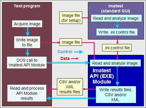
The test system interacts with the API/EXE programs through files specified in the DOS command line: the primary inputs are an image file and an INI control file (created and saved by Imatest Master during setup). The output is data files in XML or Excel-readable .CSV format. Figures can be generated and saved if desired.
Although Imatest API/EXE operates independently of Imatest Master, we strongly recommend that API/EXE users have at least one Imatest Master installation on site.
Installing Imatest API/EXE
When you purchase Imatest API/EXE or request a 30-day trial we will send you details on how to download the installation files. A typical file name is colorcheck-04-02-07.exe, where 04-02-07 is the release date. The trial expires on the same date of the following month. (This naming convention may change in future releases).
 Installation: Install the module by double-clicking on the installation file name in Windows Explorer. Then either register the module (if you purchased it) or make sure Imatest Studio or Pro is registered on your computer (for the trial version).
Registering API/EXE modules: Double-click on register_imatest.bat in the Imatest installation folder (C:\Program Files\Imatest\ in English language installations). Fill in the Name, Company, E-mail, and Password fields, keeping API in the program field, as shown on the right, then press Register.
Registration for trial version: Can be done in two ways. (1) Install Imatest and register it using the normal procedure: Click Help, Register, then fill in the fields and press Register. (2) Double-click on register_imatest.bat in the Imatest installation folder. The dialog box shown on the right appears. Fill in the fields and select Imatest in the program field, then press Register. The 30-day trial version will work with an Imatest Studio or Pro password.
Path: You should add three folders to the system path if they are not present. In Windows XP,
- Open the Control Panel.
- Double-click on System.
- Click on the Advanced tab in the System Properties window (Advanced system settings in Vista).
- Click on Environment Variables. If Matlab is installed on your system, see the Path conflicts box, below.
- Select PATH in the User variables... window.
- Click on Edit.
- Check to see if the three folders listed below are included in the Variable value field for Path.
;%ProgramFiles%\Imatest;%ProgramFiles%\Imatest\bin\win32;%ProgramFiles%\Imatest\toolbox\matlab
If they are not there, add them to the Variable value field. (You may copy and paste.)
- %ProgramFiles% is an environment variable that represents the system default program installation folder. It is equivalent to C:\Program Files in English-language installations. This folder has a different name in non-English installations, for example, C:\Programme in Deutsch, but %ProgramFiles% should be consistent for all languages. Alternatively, you may use the actual folder names.
;C:\Program Files\Imatest;C:\Program Files\Imatest\bin\win32;C:\Program Files\Imatest\toolbox\matlab (English-only)
After you add the folders, be sure the Path list is well-formed— that it consists of proper folder names separated by semicolons (;).
- Click on OK, OK, OK to close the System window.
Path conflicts
| If a different version of Matlab from the one used for Imatest (6.5.1) has been installed on your system, you may experience a path conflict that causes an error message similar to the message shown on the right— or Imatest API/EXE may simply fail to run, without returning an error message. |
|
X The procedure entry point svDoubleSclarRemW could not be
located in the dynamic link library libmwservices.dll |
|
If you receive such a message, you can try two solutions.
1. Alter the Path environment variable in System variables, located below User variables in the Environment Variables window. Be sure that the three folders listed above appear before the similar folders for the installed version of Matlab. This may involve some careful copying and pasting. Be sure to check the path carefully before you click OK.
2. Initiate API/EXE programs using the second method shown below: call a DOS BAT file, which sets the path and calls the command line. (Do this instead of directly calling the command line.) This often resolves difficult conflicts. |
Setting up API/EXE
Set up the test system (lights, camera, etc.) and photograph a test chart lighted and framed as it would be in the actual tests.
Save the image in a standard file format. It should have the same pixel count as the actual test images.
Analyze the image using (GUI-based) Imatest Master.
When the settings are correct— when the ROI (region of interest), the calculation details, and the output files and folder locations are what you need for production— press Save settings... (or Settings, Save Settings...) in the Imatest main window. This allows you to save the control information for Imatest API/EXE in a named .INI file, which can be viewed and edited with any standard text editor. Be sure to save it in a convenient, accessible folder. The contents of .ini files are largely self-explanatory. Here is a sample.
[sfr]
nht_save = 2052
nroi = 2
nwid_save = 3076
roi_mult = 1606 931 1735 1149;334 1693 466 1912
aper =
CA = Min
camera =
cyclesper = Max
cyclesper_value = 1
foclth =
gamma = 0.5
The INI file is divided into sections that start with a bracketed name. [sfr], [q13], [colorcheck], [distortion], [uniformity] are the sections for the five programs that comprise API/EXE. Of the remaining sections, only [api] (described below) affects API/EXE operation.
INI file: more detail
General settings Press Settings, API options in the main Imatest window to open a dialog box that sets options that only affect API programs— they do not affect regular Imatest operation. These options are written into the INI file.
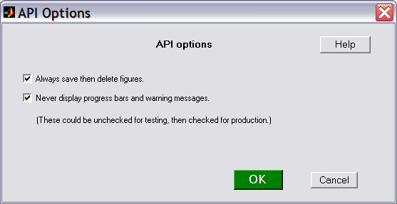
Checking Always save then delete figures makes sure all figures are closed at the end of the run, no matter what the other settings indicate.
Checking Never display progress bars and warning messages disables these graphic displays. These settings affect the contents of the following lines in the INI file.
[api]
nomsg = 1
savedel = 1
These lines can be edited in the INI file using any text editor; the API Options box is merely a convenience. Certain other options in the [imatest] section may be of interest to API users.
[imatest]
readexif = 1 (Reads EXIF data from JPEG images when set to 1; readexif = 0 turns off EXIF read.)
Figures The INI control determines which figures are generated and saved. Any figures that aren't needed they should be turned off for speed. Most are set to either Min (figure off) or Max (figure on), but some (noted in the table below), are set to 0 (figure off) or a number >= 1 (figure on, depending on conditions). These parameters can be set using a text editor, but it's usually more convenient to uncheck the appropriate boxes in the input dialog box prior to saving the INI file.
| [Section] (module) |
Plot
Name |
Plot or CSV/XML file |
save_file_list
index |
| [sfr] |
cyclesper |
MTF in cycles/(pixel or distance) |
1 |
| |
LWPH |
MTF in LW/PH |
2 |
| |
CA |
Chromatic Aberration |
3 |
| |
shannon |
Shannon capacity |
3 |
| |
|
CSV output file (detailed results) |
6 |
| |
|
XML output file (detailed results) |
7 |
| |
|
SFR_cypx.csv (summary with Cycles/pixel) |
4 |
| |
|
SFR_lwph.csv (summary with LW/PH) |
5 |
| [sqf] (SFR) |
SQF |
SQF (Subjective Quality Factor)
SQF is in its own section, but affects SFR. |
8 (in [sfr]) |
| [q13] (Stepchart) |
pltpix |
Patch levels and noise (First figure) |
1 |
| |
pltnoise |
Density response, noise, Dynamic range (Second figure) |
2 |
| |
pltallch |
Density response details (all colors) (Third figure) |
3 |
| |
|
CSV output file (detailed results) |
4 |
| |
|
XML output file (detailed results) |
6 |
| [colorcheck] |
pltones |
Grayscale tonal response and noise (First figure) |
1 |
| |
pltnoise
|
Noise detail (Second figure) |
2 |
| |
pltaberr |
a*b* error plot (Third figure) |
3 |
| |
pltcolor |
Color analysis (Fourth figure) |
4 |
| |
|
CSV output file (detailed results) |
5 |
| |
|
XML output file (detailed results) |
6 |
| [distortion] |
distfig |
Distortion figure (0 or 1) |
1 |
| |
dispcorr |
Corrected image
(if 1, displays if cropped; if 2, always displays) |
2 |
| |
outs |
Intersection point figure (0 or 1) |
3 |
| |
|
CSV output file (detailed results) |
4 |
| |
|
XML output file (detailed results) |
5 |
| [uniformity] (Light Falloff) |
contour |
Light falloff contour plots (pixels and f-stop)
(0 or 1) |
1 (pixels)
2 (f-stop) |
| |
shading |
Color shading plot (0 or 1) |
3 |
| |
detail |
Noise detail plot |
4 |
| |
|
CSV output file (detailed results) |
5 |
| |
|
XML output file (detailed results) |
6 |
The rightmost column in the above table is the index of array save_file_list, which is included in each module's section ([sfr], [q13], [colorcheck], [distortion], and [uniformity]). This index indicates which output figures and files to save. It is generated by the Save dialog box (shown on the right for SFR; Note that the order of the indices may differ from the figure.) For example,
[SFR] ...
save_file_list = 1 0 0 0 0 1 0 0
directs the SFR module to save the MTF plot in cycles/(pixel or distance) and the CSV output file that contains detailed results.
Another important variable that appears in the sections for the five modules is closefigs. If closefigs = 1, figures will be deleted after being saved. |
 |
Some specific settings
[SFR]
roi_mult contains the coordinates of the region(s) of interest, four entries per region: Left, Top, Right, Bottom (L T R B, with the number of regions specified by nroi). Units are in pixels from the top-left of the image. Note that this is different from the order displayed on the SFR Edge/MTF figure: L R T B.
DOS Command line call
Imatest API/EXE programs are initiated by one of two methods.
The first and simplest method is a direct DOS command line call, which has the following form.
c:\program files\imatest\sfr.exe param-1 param-2 param-3 param-4 param-5
Ths second method is to create and call to a DOS BAT file, which sets the path and calls a DOS command line. This may be needed when the first method fails, for example, when a path conflict is difficult to resolve (which may happen in installations that contain newer versions of Matlab than the one used to compile Imatest). The call to the BAT file has the form,
pathname\batfilename.bat
where batfilename.bat contains lines of the following form.
path="%ProgramFiles%\Imatest;%ProgramFiles%\Imatest\bin\win32;%ProgramFiles%\Imatest\toolbox\matlab;%path%"
c:\program files\imatest\sfr.exe param-1 param-2 param-3 param-4 param-5
The first three parameters (param-1 − param-3) are required. The fourth is optional but strongly recommended and the fifth is optional. The program name and parameters 2-5 should contain full path names to minimize the likelihood of error.
| Param-1 |
-1 closes the DOS window and all figures when the program terminates. For normal operation of API/EXE programs. -2, -3, and -4 are for debugging.
-2 keeps the DOS window open after the program terminates.
-3 closes the DOS window and all figures when the program terminates and opens the error log file if an error is detected.
-4 keeps the DOS window open after the program terminates and opens the error log file if an error is detected. |
| Param-2 |
Image file name. The full path name should be used, e.g.,"c:\program files\imatest\API\Stepchart_DR_Canon_G2.JPG"in the example below |
| Param-3 |
Folder where the API/EXE and other programs are located. ( "c:\program files\imatest" in the example below, which is typical of English language systems). The C:\Program files folder has different names in different languages, for example, C:\Programme in German. The name can be viewed by entering set %ProgramFiles% in a DOS window.) |
| Param-4 (optional*) |
.ini control file name. If omitted, it defaults to imatest.ini in the same directory as sfr.exe."c:\program files\imatest\API\stepchart_DR_canon_G2.ini" in the example below.) We strongly recommend including it. |
| Param-5 (optional) |
folder where results are written. If omitted, it defaults to subfolder Results in the directory that contains the image file. ( "c:\program files\imatest\API\Results" in the example below.) |
*Always use these fields until further notice. |
We may add additional parameter-value pairs on user request.
If field names contain blanks, they should be enclosed in quotation marks ("). We recommend always enclosing all fields, including the program call, in quotation marks, except for parameter 1 (which must be -1). Example:
"c:\program files\imatest\stepchart.exe" -1 "c:\program files\imatest\API\Stepchart_DR_Canon_G2.JPG" "c:\program files\imatest" "c:\program files\imatest\API\stepchart_DR_canon_G2.ini" "c:\program files\imatest\API\Results"
Calling API/EXE from Matlab
DOS commands can be called from Matlab by statements of the form,
dos('command')
system('command')
!command — or
—
!command & (opens and displays results in a separate DOS window)
where command is a dos command string, which can take the form shown in the example above. Dos or system are recommended.
If you are running Matlab 6.5.1 (the same version used by Imatest), a direct DOS command line call (illustrated above), should work fine. But if you are using a newer version of Matlab (7+), the second method, a call to a DOS BAT file (also illustrated above), may be required to avoid path issues. The following code creates and runs a bat file (sfr_batest.bat). It has been tested with Matlab 7.4.0 (R2007a).
fbat = fopen('c:\imatest\matlab\sfr_battest.bat','wt');
fprintf(fbat,['path="%%ProgramFiles%%\\Imatest;%%ProgramFiles%%\\Imatest\\bin\\win32;' ...
'%%ProgramFiles%%\\Imatest\\toolbox\\matlab;%%path%%"\n']);
fprintf(fbat,['"c:\\program files\\imatest\\sfr.exe" -1 "c:\\imatest\\data_SFR\\Canon_17-40_24_f8_C1_1409.jpg" ' ...
'"c:\\program files\\imatest" "c:\\Imatest\\matlab\\Results\\Canon1740_ctr.ini"\n']);
fclose(fbat);
dos('c:\imatest\matlab\sfr_battest.bat');
% !c:\imatest\matlab\sfr_battest.bat &
%% and \\ are escape sequences that cause single % and \ characters to be written. File sfr_battest.bat contains the following two lines:
path="%ProgramFiles%\Imatest;%ProgramFiles%\Imatest\bin\win32;%ProgramFiles%\Imatest\toolbox\matlab;%path%"
"c:\program files\imatest\sfr.exe" -1 "c:\imatest\data_SFR\Canon_17-40_24_f8_C1_1409.jpg" "c:\program files\imatest" "c:\Imatest\matlab\Results\Canon1740_ctr.ini"
Testing Imatest API/EXE
Several test files (image files, INI control files, and DOS BAT files) are available for testing and verifying API/EXE installations. The image files can also be used with Imatest Master. Right-click on the file names in the table below to download the files. We recommend saving them in subfolder API of the Imatest installation folder: C:\Program files\Imatest\API (in English language installations) or in the equivalent in other languages (for example, C:\Programme\... in German). For testing we recommend setting the first parameter in the DOS call to -4 (keep the DOS window open and display the error log if an error occurs).
Downloadable test images |
Module |
Image file |
INI & BAT files |
Description |
|
|
|
Webcam image of high and medium contrast custom charts created by Test Charts and printed on an Epson R2400 printer: these can have larger regions of interest (ROIs) than the ISO 12233 chart below. |
|
|
Webcam image of ISO 12233 chart. At this distance the available regions of interest are very small. |
|
|
|
Webcam image of the Kodak Q-14 grayscale and GretagMacbeth ColorChecker. |
|
|
stepchart_DR_canon_G2.ini
stepchart_DR_canon_G2.bat |
Image of the Stouffer T4110 transmission test chart taken with the Canon Powershot G2. Excellent dynamic range measurement. |
|
|
Webcam image of the Kodak Q-14 grayscale and GretagMacbeth ColorChecker. |
|
|
12-patch OECF chart (for API and Imatest Master only ). Available from Applied Image. |
|
|
Image of Kodak Q-14 chart with "black hole" cavity for measuring veiling glare (susceptibility to lens flare) |
|
|
|
Webcam image of distortion grid. |
|
|
|
Image of nearly uniformly illuminated surface taken with the Canon 10-22mm lens on the EOS-20D, f/4.5, 22mm, ISO 1600. |
To use these test files,
- Make any necessary changes to the saved ini and bat files using a text editor. You'll need to update folder names if Imatest is installed in a folder other than C:\Program files\Imatest or the test files (above) have been saved in a folder other than C:\Program files\Imatest\API. You only need to edit folder names in the appropriate section of the ini file, which follows the module name enclosed in brackets: [sfr], [colorcheck], [q13] (for Stepchart), [distortion], or [uniformity] (for Light Falloff).
- Open a DOS window (Start, Run..., cmd; Start, All Programs >, Accessories >, Command Prompt).
- Change to the directory where the files are located. Typically, enter
cd C:\Program files\Imatest\API.
- Run the bat file by entering the file name, omitting the bat-extension. For example,
stepchart_DR_canon_G2
- Verify the results by looking in the folder where resuts are stored, typically subfolder Results of the folder that contains the image, ini, and bat files. If you found errors that aren't obvious and aren't covered in the Troubleshooting page, please contact us.
Error handling
Imatest API/EXE modules return a value of 0 if they terminate correctly or 1 or larger if they terminate in error.
If an error is detected, a message is
- appended to the error log file, which has the name of the form module.log (sfr.log, colorcheck.log, stepchart.log, distortion.log, or uniformity.log), and is is located in %APPDATA%\Imatest.
- written to the CSV and/or XML file that would otherwise contain the results of the run. For the example above,
"c:\program files\imatest\stepchart.exe" -1 "c:\program files\imatest\API\Stepchart_DR_Canon_G2.JPG" "c:\program files\imatest"
"c:\program files\imatest\API\stepchart_DR_canon_G2.ini" "c:\program files\imatest\API\Results"
if a CSV output file were called for, it would be c:\program files\imatest\API\Results\Stepchart_DR_Canon_G2_summary.csv ;
if an XML output file were called for, it would be c:\program files\imatest\API\Results\Stepchart_DR_Canon_G2.xml .
APPDATA is a DOS environment variable whose value can be found by opening a DOS window (you can double-click start-dos.bat in the Imatest folder), and typing
set APPDATA (Returns the folder name corresponding to APPDATA)
--or--
dir "%APPDATA%\Imatest"
APPDATA has values of the form
- C:\Users\your name\AppData\Roaming in Windows Vista.
- C:\Documents and Settings\your name\Application Data in Windows XP.
To facilitate debugging, the log file will be opened in Notepad if an error is detected and the first parameter of the API/EXE DOS call is -3 or -4.
Lines in the log file have the format,
[Date Time], file_name, error_message
Example:
[05-May-2007 23:34:08], c:\Imatest\data_distortion\distgrid101.jpg, Inconsistent Vert lines 17 det.; 18 avg. Incomplete line?
We are constantly working to improve the robustness of Imatest algorithms to minimize the occurrences of errors, which are typically caused by poor region (ROI) selections or poor quality images.
Imatest IT/EXE instructions
Running Imatest IT/EXE
How Imatest IT/EXE works
Imatest IT/EXE is a set of standalone programs initiated by DOS calls from the test system. The programs have the same functionality as the corresponding modules in Imatest Master, but they operate without user intervention, making them suitable for use in automated systems. They are represented by the blue box in the lower right of the figure below.
The test system interacts with the IT/EXE programs through files specified in the DOS command line: the primary inputs are an image file and an INI control file (created and saved by Imatest Master during setup). The output is data files in XML or Excel-readable .CSV format. Figures can be generated and saved if desired.
Although Imatest IT/EXE operates independently of Imatest Master, we strongly recommend that IT/EXE users have at least one Imatest Master installation on site.
Installing Imatest IT/EXE
When you purchase Imatest IT/EXE or request a 30-day trial we will send you details on how to download the installation files. A typical file name is colorcheck-04-02-07.exe, where 04-02-07 is the release date. The trial expires on the same date of the following month. (This naming convention may change in future releases).
Installation: Install the module by double-clicking on the installation file name in Windows Explorer. Then either register the module (if you purchased it) or make sure Imatest Studio or Pro is registered on your computer (for the trial version).
Registering IT/EXE modules: Double-click on register_imatest.bat in the Imatest installation folder (C:\Program Files\Imatest\ in English language installations). Fill in the Name, Company, E-mail, and Password fields, keeping IT in the program field, as shown on the right, then press Register.
Registration for trial version: Can be done in two ways. (1) Install Imatest and register it using the normal procedure: Click Help, Register, then fill in the fields and press Register. (2) Double-click on register_imatest.bat in the Imatest installation folder. The dialog box shown on the right appears. Fill in the fields and select Imatest in the program field, then press Register. The 30-day trial version will work with an Imatest Studio or Pro password.
Path: You should add three folders to the system path if they are not present. In Windows XP,
- Open the Control Panel.
- Double-click on System.
- Click on the Advanced tab in the System Properties window (Advanced system settings in Vista).
- Click on Environment Variables. If Matlab is installed on your system, see the Path conflicts box, below.
- Select PATH in the User variables... window.
- Click on Edit.
- Check to see if the three folders listed below are included in the Variable value field for Path.
;%ProgramFiles%\Imatest;%ProgramFiles%\Imatest\bin\win32;%ProgramFiles%\Imatest\toolbox\matlab
If they are not there, add them to the Variable value field. (You may copy and paste.)
- %ProgramFiles% is an environment variable that represents the system default program installation folder. It is equivalent to C:\Program Files in English-language installations. This folder has a different name in non-English installations, for example, C:\Programme in Deutsch, but %ProgramFiles% should be consistent for all languages. Alternatively, you may use the actual folder names.
;C:\Program Files\Imatest;C:\Program Files\Imatest\bin\win32;C:\Program Files\Imatest\toolbox\matlab (English-only)
After you add the folders, be sure the Path list is well-formed— that it consists of proper folder names separated by semicolons (;).
- Click on OK, OK, OK to close the System window.
Path conflicts
| If a different version of Matlab from the one used for Imatest (6.5.1) has been installed on your system, you may experience a path conflict that causes an error message similar to the message shown on the right— or Imatest IT/EXE may simply fail to run, without returning an error message. |
|
X The procedure entry point svDoubleSclarRemW could not be
located in the dynamic link library libmwservices.dll |
|
If you receive such a message, you can try two solutions.
1. Alter the Path environment variable in System variables, located below User variables in the Environment Variables window. Be sure that the three folders listed above appear before the similar folders for the installed version of Matlab. This may involve some careful copying and pasting. Be sure to check the path carefully before you click OK.
2. Initiate IT/EXE programs using the second method shown below: call a DOS BAT file, which sets the path and calls the command line. (Do this instead of directly calling the command line.) This often resolves difficult conflicts. |
Setting up IT/EXE
Set up the test system (lights, camera, etc.) and photograph a test chart lighted and framed as it would be in the actual tests.
Save the image in a standard file format. It should have the same pixel count as the actual test images.
Analyze the image using (GUI-based) Imatest Master.
When the settings are correct— when the ROI (region of interest), the calculation details, and the output files and folder locations are what you need for production— press Save settings... (or Settings, Save Settings...) in the Imatest main window. This allows you to save the control information for Imatest IT/EXE in a named .INI file, which can be viewed and edited with any standard text editor. Be sure to save it in a convenient, accessible folder. The contents of .ini files are largely self-explanatory. Here is a sample.
[sfr]
nht_save = 2052
nroi = 2
nwid_save = 3076
roi_mult = 1606 931 1735 1149;334 1693 466 1912
aper =
CA = Min
camera =
cyclesper = Max
cyclesper_value = 1
foclth =
gamma = 0.5
The INI file is divided into sections that start with a bracketed name. [sfr], [q13], [colorcheck], [distortion], [uniformity] are the sections for the five programs that comprise IT/EXE. Of the remaining sections, only [api] (described below) affects IT/EXE operation.
INI file: more detail
General settings Press Settings, IT options in the main Imatest window to open a dialog box that sets options that only affect IT programs— they do not affect regular Imatest operation. These options are written into the INI file.
Checking Always save then delete figures makes sure all figures are closed at the end of the run, no matter what the other settings indicate.
Checking Never display progress bars and warning messages disables these graphic displays. These settings affect the contents of the following lines in the INI file.
[api]
nomsg = 1
savedel = 1
These lines can be edited in the INI file using any text editor; the IT Options box is merely a convenience. Certain other options in the [imatest] section may be of interest to IT users.
[imatest]
readexif = 1 (Reads EXIF data from JPEG images when set to 1; readexif = 0 turns off EXIF read.)
Figures The INI control determines which figures are generated and saved. Any figures that aren't needed they should be turned off for speed. Most are set to either Min (figure off) or Max (figure on), but some (noted in the table below), are set to 0 (figure off) or a number >= 1 (figure on, depending on conditions). These parameters can be set using a text editor, but it's usually more convenient to uncheck the appropriate boxes in the input dialog box prior to saving the INI file.
| [Section] (module) |
Plot
Name |
Plot or CSV/XML file |
save_file_list
index |
| [sfr] |
cyclesper |
MTF in cycles/(pixel or distance) |
1 |
| |
LWPH |
MTF in LW/PH |
2 |
| |
CA |
Chromatic Aberration |
3 |
| |
shannon |
Shannon capacity |
3 |
| |
|
CSV output file (detailed results) |
6 |
| |
|
XML output file (detailed results) |
7 |
| |
|
SFR_cypx.csv (summary with Cycles/pixel) |
4 |
| |
|
SFR_lwph.csv (summary with LW/PH) |
5 |
| [sqf] (SFR) |
SQF |
SQF (Subjective Quality Factor)
SQF is in its own section, but affects SFR. |
8 (in [sfr]) |
| [q13] (Stepchart) |
pltpix |
Patch levels and noise (First figure) |
1 |
| |
pltnoise |
Density response, noise, Dynamic range (Second figure) |
2 |
| |
pltallch |
Density response details (all colors) (Third figure) |
3 |
| |
|
CSV output file (detailed results) |
4 |
| |
|
XML output file (detailed results) |
6 |
| [colorcheck] |
pltones |
Grayscale tonal response and noise (First figure) |
1 |
| |
pltnoise
|
Noise detail (Second figure) |
2 |
| |
pltaberr |
a*b* error plot (Third figure) |
3 |
| |
pltcolor |
Color analysis (Fourth figure) |
4 |
| |
|
CSV output file (detailed results) |
5 |
| |
|
XML output file (detailed results) |
6 |
| [distortion] |
distfig |
Distortion figure (0 or 1) |
1 |
| |
dispcorr |
Corrected image
(if 1, displays if cropped; if 2, always displays) |
2 |
| |
outs |
Intersection point figure (0 or 1) |
3 |
| |
|
CSV output file (detailed results) |
4 |
| |
|
XML output file (detailed results) |
5 |
| [uniformity] (Light Falloff) |
contour |
Light falloff contour plots (pixels and f-stop)
(0 or 1) |
1 (pixels)
2 (f-stop) |
| |
shading |
Color shading plot (0 or 1) |
3 |
| |
detail |
Noise detail plot |
4 |
| |
|
CSV output file (detailed results) |
5 |
| |
|
XML output file (detailed results) |
6 |
The rightmost column in the above table is the index of array save_file_list, which is included in each module's section ([sfr], [q13], [colorcheck], [distortion], and [uniformity]). This index indicates which output figures and files to save. It is generated by the Save dialog box (shown on the right for SFR; Note that the order of the indices may differ from the figure.) For example,
[SFR] ...
save_file_list = 1 0 0 0 0 1 0 0
directs the SFR module to save the MTF plot in cycles/(pixel or distance) and the CSV output file that contains detailed results.
Another important variable that appears in the sections for the five modules is closefigs. If closefigs = 1, figures will be deleted after being saved. |
|
Some specific settings
[SFR]
roi_mult contains the coordinates of the region(s) of interest, four entries per region: Left, Top, Right, Bottom (L T R B, with the number of regions specified by nroi). Units are in pixels from the top-left of the image. Note that this is different from the order displayed on the SFR Edge/MTF figure: L R T B.
DOS Command line call
Imatest IT/EXE programs are initiated by one of two methods.
The first and simplest method is a direct DOS command line call, which has the following form.
c:\program files\imatest\sfr.exe param-1 param-2 param-3 param-4 param-5
Ths second method is to create and call to a DOS BAT file, which sets the path and calls a DOS command line. This may be needed when the first method fails, for example, when a path conflict is difficult to resolve (which may happen in installations that contain newer versions of Matlab than the one used to compile Imatest). The call to the BAT file has the form,
pathname\batfilename.bat
where batfilename.bat contains lines of the following form.
path="%ProgramFiles%\Imatest;%ProgramFiles%\Imatest\bin\win32;%ProgramFiles%\Imatest\toolbox\matlab;%path%"
c:\program files\imatest\sfr.exe param-1 param-2 param-3 param-4 param-5
The first three parameters (param-1 − param-3) are required. The fourth is optional but strongly recommended and the fifth is optional. The program name and parameters 2-5 should contain full path names to minimize the likelihood of error.
| Param-1 |
-1 closes the DOS window and all figures when the program terminates. For normal operation of IT/EXE programs. -2, -3, and -4 are for debugging.
-2 keeps the DOS window open after the program terminates.
-3 closes the DOS window and all figures when the program terminates and opens the error log file if an error is detected.
-4 keeps the DOS window open after the program terminates and opens the error log file if an error is detected. |
| Param-2 |
Image file name. The full path name should be used, e.g.,"c:\program files\imatest\IT\Stepchart_DR_Canon_G2.JPG"in the example below |
| Param-3 |
Folder where the IT/EXE and other programs are located. ( "c:\program files\imatest" in the example below, which is typical of English language systems). The C:\Program files folder has different names in different languages, for example, C:\Programme in German. The name can be viewed by entering set %ProgramFiles% in a DOS window.) |
| Param-4 (optional*) |
.ini control file name. If omitted, it defaults to imatest.ini in the same directory as sfr.exe."c:\program files\imatest\IT\stepchart_DR_canon_G2.ini" in the example below.) We strongly recommend including it. |
| Param-5 (optional) |
folder where results are written. If omitted, it defaults to subfolder Results in the directory that contains the image file. ( "c:\program files\imatest\IT\Results" in the example below.) |
*Always use these fields until further notice. |
We may add additional parameter-value pairs on user request.
If field names contain blanks, they should be enclosed in quotation marks ("). We recommend always enclosing all fields, including the program call, in quotation marks, except for parameter 1 (which must be -1). Example:
"c:\program files\imatest\stepchart.exe" -1 "c:\program files\imatest\IT\Stepchart_DR_Canon_G2.JPG" "c:\program files\imatest" "c:\program files\imatest\IT\stepchart_DR_canon_G2.ini" "c:\program files\imatest\IT\Results"
Calling IT/EXE from Matlab
DOS commands can be called from Matlab by statements of the form,
dos('command')
system('command')
!command — or
—
!command & (opens and displays results in a separate DOS window)
where command is a dos command string, which can take the form shown in the example above. Dos or system are recommended.
If you are running Matlab 6.5.1 (the same version used by Imatest), a direct DOS command line call (illustrated above), should work fine. But if you are using a newer version of Matlab (7+), the second method, a call to a DOS BAT file (also illustrated above), may be required to avoid path issues. The following code creates and runs a bat file (sfr_batest.bat). It has been tested with Matlab 7.4.0 (R2007a).
fbat = fopen('c:\imatest\matlab\sfr_battest.bat','wt');
fprintf(fbat,['path="%%ProgramFiles%%\\Imatest;%%ProgramFiles%%\\Imatest\\bin\\win32;' ...
'%%ProgramFiles%%\\Imatest\\toolbox\\matlab;%%path%%"\n']);
fprintf(fbat,['"c:\\program files\\imatest\\sfr.exe" -1 "c:\\imatest\\data_SFR\\Canon_17-40_24_f8_C1_1409.jpg" ' ...
'"c:\\program files\\imatest" "c:\\Imatest\\matlab\\Results\\Canon1740_ctr.ini"\n']);
fclose(fbat);
dos('c:\imatest\matlab\sfr_battest.bat');
% !c:\imatest\matlab\sfr_battest.bat &
%% and \\ are escape sequences that cause single % and \ characters to be written. File sfr_battest.bat contains the following two lines:
path="%ProgramFiles%\Imatest;%ProgramFiles%\Imatest\bin\win32;%ProgramFiles%\Imatest\toolbox\matlab;%path%"
"c:\program files\imatest\sfr.exe" -1 "c:\imatest\data_SFR\Canon_17-40_24_f8_C1_1409.jpg" "c:\program files\imatest" "c:\Imatest\matlab\Results\Canon1740_ctr.ini"
Testing Imatest IT/EXE
Several test files (image files, INI control files, and DOS BAT files) are available for testing and verifying IT/EXE installations. The image files can also be used with Imatest Master. Right-click on the file names in the table below to download the files. We recommend saving them in subfolder IT of the Imatest installation folder: C:\Program files\Imatest\IT (in English language installations) or in the equivalent in other languages (for example, C:\Programme\... in German). For testing we recommend setting the first parameter in the DOS call to -4 (keep the DOS window open and display the error log if an error occurs).
Downloadable test images |
Module |
Image file |
INI & BAT files |
Description |
|
|
|
Webcam image of high and medium contrast custom charts created by Test Charts and printed on an Epson R2400 printer: these can have larger regions of interest (ROIs) than the ISO 12233 chart below. |
|
|
Webcam image of ISO 12233 chart. At this distance the available regions of interest are very small. |
|
|
|
Webcam image of the Kodak Q-14 grayscale and GretagMacbeth ColorChecker. |
|
|
stepchart_DR_canon_G2.ini
stepchart_DR_canon_G2.bat |
Image of the Stouffer T4110 transmission test chart taken with the Canon Powershot G2. Excellent dynamic range measurement. |
|
|
Webcam image of the Kodak Q-14 grayscale and GretagMacbeth ColorChecker. |
|
|
12-patch OECF chart (for IT and Imatest Master only ). Available from Applied Image. |
|
|
Image of Kodak Q-14 chart with "black hole" cavity for measuring veiling glare (susceptibility to lens flare) |
|
|
|
Webcam image of distortion grid. |
|
|
|
Image of nearly uniformly illuminated surface taken with the Canon 10-22mm lens on the EOS-20D, f/4.5, 22mm, ISO 1600. |
To use these test files,
- Make any necessary changes to the saved ini and bat files using a text editor. You'll need to update folder names if Imatest is installed in a folder other than C:\Program files\Imatest or the test files (above) have been saved in a folder other than C:\Program files\Imatest\IT. You only need to edit folder names in the appropriate section of the ini file, which follows the module name enclosed in brackets: [sfr], [colorcheck], [q13] (for Stepchart), [distortion], or [uniformity] (for Light Falloff).
- Open a DOS window (Start, Run..., cmd; Start, All Programs >, Accessories >, Command Prompt).
- Change to the directory where the files are located. Typically, enter
cd C:\Program files\Imatest\IT.
- Run the bat file by entering the file name, omitting the bat-extension. For example,
stepchart_DR_canon_G2
- Verify the results by looking in the folder where resuts are stored, typically subfolder Results of the folder that contains the image, ini, and bat files. If you found errors that aren't obvious and aren't covered in the Troubleshooting page, please contact us.
Error handling
Imatest IT/EXE modules return a value of 0 if they terminate correctly or 1 or larger if they terminate in error.
If an error is detected, a message is
- appended to the error log file, which has the name of the form module.log (sfr.log, colorcheck.log, stepchart.log, distortion.log, or uniformity.log), and is is located in %APPDATA%\Imatest.
- written to the CSV and/or XML file that would otherwise contain the results of the run. For the example above,
"c:\program files\imatest\stepchart.exe" -1 "c:\program files\imatest\IT\Stepchart_DR_Canon_G2.JPG" "c:\program files\imatest"
"c:\program files\imatest\IT\stepchart_DR_canon_G2.ini" "c:\program files\imatest\IT\Results"
if a CSV output file were called for, it would be c:\program files\imatest\IT\Results\Stepchart_DR_Canon_G2_summary.csv ;
if an XML output file were called for, it would be c:\program files\imatest\IT\Results\Stepchart_DR_Canon_G2.xml .
APPDATA is a DOS environment variable whose value can be found by opening a DOS window (you can double-click start-dos.bat in the Imatest folder), and typing
set APPDATA (Returns the folder name corresponding to APPDATA)
--or--
dir "%APPDATA%\Imatest"
APPDATA has values of the form
- C:\Users\your name\AppData\Roaming in Windows Vista.
- C:\Documents and Settings\your name\Application Data in Windows XP.
To facilitate debugging, the log file will be opened in Notepad if an error is detected and the first parameter of the IT/EXE DOS call is -3 or -4.
Lines in the log file have the format,
[Date Time], file_name, error_message
Example:
[05-May-2007 23:34:08], c:\Imatest\data_distortion\distgrid101.jpg, Inconsistent Vert lines 17 det.; 18 avg. Incomplete line?
We are constantly working to improve the robustness of Imatest algorithms to minimize the occurrences of errors, which are typically caused by poor region (ROI) selections or poor quality images.
Maskfill
Removes features that interfere with Imatest measurements
Introduction to Maskfill
Imatest Maskfill (mask and fill) is a standalone program for removing features in test images that interfere with Imatest analysis. A typical image is shown below: it has passed through a fiber optic bundle that adds a "honeycomb" interfering pattern. Imatest modules such as SFR will often fail with this pattern. Maskfill removes the honeycomb pattern so that Imatest modules can run properly and produce correct results.
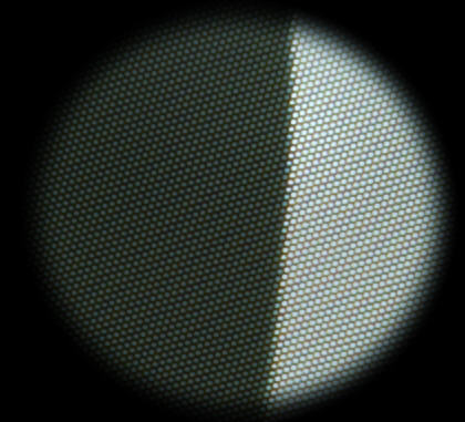
SFR slanted-edge test image with interference:
used as the Uncorrected image
Please contact us if you are interested in purchasing Maskfill.
To run Maskfill, you'll need an image of a uniform, featureless surface (white or gray preferred) taken with the same interfering pattern as the test image(s). This pattern, called the Mask input, is used for creating a mask (the first step in Maskfill).
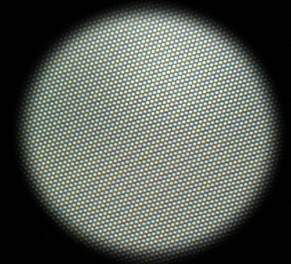
Image of plain surface:
used as the Mask input.
Must be the same pixel size and alignment as the uncorrected image.
Instructions
- Install Maskfill by double-clicking on the install file, which has a name like Maskfill-1.n.exe (where n is a number). Imatest Master should be installed first. Maskfill is installed into the Imatest program file (C:\program files\Imatest in English language installations).
- Acquire one or more test target images and one image of a plain, unstructured surface (the mask input). The image of the plain surface is used for making the mask: it should have the same interfering pattern as the test images. Save the images in standard file formats (TIFF, PNG, JPEG (high quality), etc.). The mask input image and the test target images must have the same alignment and the same pixel size.
- Open Maskfill by clicking on the icon on the Windows wallpaper (background) that is installed with the program, or by opening Windows Explorer and clicking on Maskfill in the Imatest program file. The following screen (shown reduced to 75% of the original size) appears. This window can be maximized to enhance the resolution of the images.
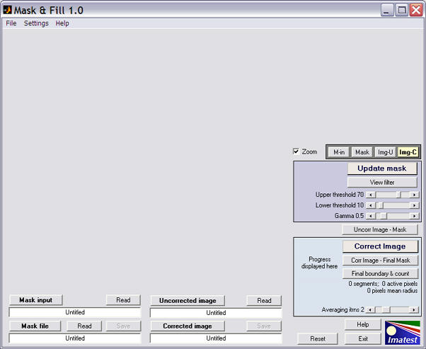
Maskfill: initial display
- The Maskfill window. Most of the left side is reserved for the main image. The lower-left contains the Display/Read/Save area for the four images processed by Maskfill. The four file names (the long white boxes) are all Untitled when Maskfill is started.
- The Mask input: the image of a plain, unstuctured surface used to create the mask: the second of the images above.
- The Mask, which can be read in or created using controls in the blue area on the right. Shown below.
- The Uncorrected image, i.e., with interference: The first of the images above.
- The Corrected image, i.e., with interference removed. Shown below.
The Read buttons above all files but Corrected image open dialog boxes for reading the files, which will be displayed after they are read. The Save buttons above Mask file and Corrected image save the files calculated by Maskfill. The file names replace "Untitled" in the long white boxes. The buttons on the upper right ( M-in, Mask, Img-U, Img-C )can be used to display one of these four images on the upper right.
The large buttons above all four file boxes display the files. If Mask input or Uncorrected image files have not been read in, the dialog box for reading them will be displayed. If Mask file hasn't been calculated or read, it will be calculated if the Mask input file has been read in. Here is the display after Mask input (the image of the plain, unstructured surface) has been read. The long file name box for the displayed image is highlighted in yellow.
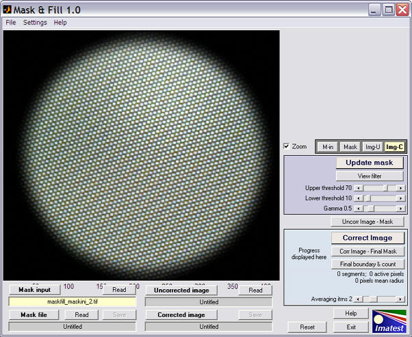
Display of Mask input image
- Read the Mask input image. This is the image of a plain, unstuctured surface used to create the mask.
- Create the mask. The light blue box to the right of the image contains the controls for creating the mask. Three sliders control the appearance of the mask.
- Upper threshold (default 70) is a variable threshold, that changes with the average (lowpass-filtered) image brightness. Increasing it shrinks the light areas of the mask.
- Lower threshold (default 10) is an absolute threshold, used so that noise in dark areas is not included in the mask.
- Gamma (default 0.5) is the encoding gamma used for creating the Mask input image file. It should be 0.5 for most standard image files (with color spaces such as sRGB, etc.) designed for display at gamma = 1.8 or 2.2. (It doesn't have to be precise.) It should be set to 1 for linear files, i.e., files created without gamma-encoding. It affects the uniformity of the mask.
When you've adjusted these sliders, click Update mask to create the mask, which will appear in the main window. All desired areas should be a part of the mask (i.e., white in the B&W mask image). In this case, we want each fiber to be distinct: we don't want them to be merged. Since the mask calculation is very fast we recommend tryuing out the slider settings to see what they do.
Displays can be zoomed in or out if the Zoom box is checked. You can zoom in by clicking on the image or drawing a box with the mouse. You zoom out by double-clicking on the image. A zoomed portion of the mask is shown below.
Mask image, zoomed
The View filter button displays the lowpass-filtered version of the Mask input image, used for the Upper (variable) threshold.
- Read the Uncorrected image. This is the image that must be corrected before it can be entered into Imatest. The first image on this page is an example.
- Correct the image. The cyan box on the lower right contains the correction controls. The only adjustment is the slider that sets the maximum averaging iterations (the number of passes where adjacent pixels inside the mask (white regions) are averaged). For this image there was little improvement for more than two passes.
Press the Correct image button to perform the correction. The correction iteratively grows the image in the masked areas (white in the mask image) into adjacent unmasked areas (black in the mask image) until convergence is detected. It can be somewhat slow, but it may be sped up in future releases. The corrected image appears in the window.
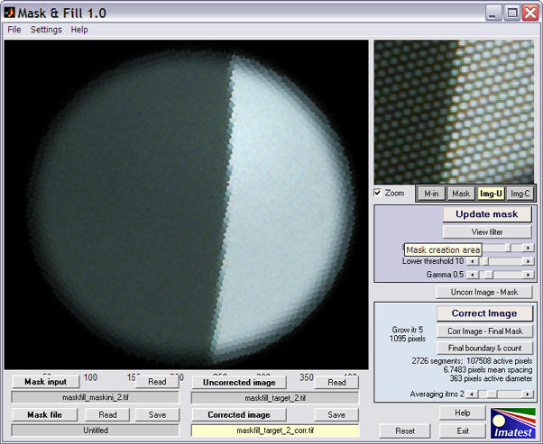
A zoomed view of the uncorrected image has been displayed in the upper-right for comparision. The Maskfill window also displays several interesting results: the number of segments (i.e., distince fiber light sources), the number of active pixels (inside the final mask), the mean spacing between the pixels (valid only for the hexagonal "honeycomb" pattern), and the diameter of the circle (4 pixels less than the measured mean of ymax-ymin and xmax-xmin for the final image boundaries).
The two buttons below Correct Image can be used to produce interesting displays. The first, Corr Image - Final Mask, shows only the active portion of the final corrected image, with the unmasked part as white. It is useful for visualizing the final mask boundary.
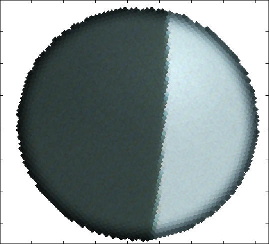
Corr Image - Final Mask corrected image, unmasked area in white
The second button, Final boundary & count, shows the final boundary and the image used to count the number of segments (light sources, i.e., active fibers in the fiber optic bundle). By zooming in (or maximizing the window), you can check to see that no individual light sources were missed or no two sources were merged. The following shows a zoom of the image. The squares represent single pixels. They are uneven in size because the Matlab display is not anti-aliased.
Final boundary & count zoomed in, showing individual light sources
- Save the corrected image by pressing the Save button for the Corrected image. TIFF (uncompressed), PNG (losselessly compressed), or high quality JPEG are the preferred image formats. The image in the illustration is suitable for analysis by Imatest SFR.
This image runs nicely in Imatest SFR. Here is a sample.
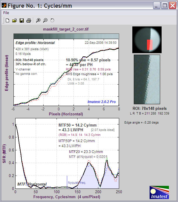
Imatest SFR results for image processed by Maskfill.
Appendix
Cross-reference tables
Tables to help you navigate Imatest
Imatest is a complex, rich application involving a great many image quality factors, modules, and test charts. The tables below, sorted by Quality Factor, Module, and Test chart are designed to help navigate the site. A Table of contents is also available.
Suppliers
Sorted by image quality factors
Image quality factors have their own page. A brief list of recommended test charts is given in the FAQ.
| Quality factor |
Charts |
Module |
Comments |
Camera, lens |
| Color accuracy |
GretagMacbeth ColorChecker (24-patch) |
Colorcheck, Multicharts |
|
| IT8.7 |
Multicharts |
|
| ColorChecker SG |
Multicharts |
Imatest Master only |
| Custom "pie" charts |
Multicharts |
Imatest Master only |
| Dynamic range, Tonal response, Contrast |
Step charts |
Stepchart |
Transmissive charts such as the Stouffer T4110 recommended for older Dynamic Range measurement. |
| Reflective step charts |
Dynamic Range |
More convenient for measuring DR than Stepchart because it doesn't require a transmission chart. |
| Special charts: ISO-16067-1, QA-62, ISO-14524
OECF, ISO-15739
Noise, 20-patch OECF charts |
Stepchart |
Imatest Master only. Most are available from Applied Image. |
| ColorChecker, ColorChecker SG, IT8.7, Step Charts |
Multicharts |
|
| Exposure accuracy |
Step chart (reflective) such as the Kodak Q-13/Q-14 |
Stepchart |
|
| GretagMacbeth ColorChecker |
Colorcheck |
|
| Lateral chromatic aberration |
Slanted edge (can be printed from Test Charts) |
SFR
Rescharts SFR |
Printable by Test Charts |
| ISO 12233, Applied Image QA-77 |
Printed on photographic media |
| Lens distortion |
Square or rectangular grid or checkerboard (can be printed from Test Charts or displayed with Screen Patterns), SFRplus chart |
Distortion
SFRplus
|
Grid or checkerboard printable by Test Charts. |
| Light falloff, vignetting |
plain, uniformly lit surface |
Lightfall |
Best: Screen Patterns with LCD flat screen. |
| Noise |
Step charts such as the Kodak Q-13/Q-14 |
Stepchart |
|
| GretagMacbeth ColorChecker |
Colorcheck |
|
| Sharpness (MTF) |
Slanted-edge (can be printed from Test Charts)
ISO 12233, Applied Image QA-77
Log Frequency chart
Log F-Contrast chart
Star chart |
SFR
Rescharts SFR
Log Frequency
Log F-Contrast
Star Chart |
Printable by Test Charts
Printed on photographic media
Printable by Test Charts
Printable by Test Charts
'' or purchase from Image Engineering |
| SFRplus chart (highly automated) |
SFRplus |
Printable or purchase from the Imatest store |
Sorted by module
Modules are listed on the Tour page.
| Module |
Quality factor |
Charts |
Comments |
| Colorcheck |
Color accuracy, Tonal response, Contrast, |
GretagMacbeth ColorChecker |
|
| Distortion |
Lens distortion |
Square or rectangular grid |
|
| Lightfall |
Light falloff, vignetting |
plain, uniformly lit surface |
|
| Multicharts |
Color accuracy, Tonal response, Contrast |
GretagMacbeth ColorChecker, IT8.7, ColorChecker SG, Step charts, special charts: ISO-16067-1, QA-62, EIA Grayscale, ISO-14524
OECF, ISO-15739
Noise, 20-patch OECF charts |
ColorChecker SG, Step charts, special charts: Imatest Master only |
| SFR, Rescharts SFR |
Sharpness (MTF), Lateral chromatic aberration |
Slanted-edge (printable by Test Charts), ISO 12233, Applied Image QA-77 |
Also measures Subjective Quality Factor (SQF). |
| SFRplus |
Sharpness (MTF), Lateral chromatic aberration, Tonal response, Lens distortion |
SFRplus chart |
Highly automated module: no manual ROI selection. Chart available from the Imatest store. |
| Stepchart |
Tonal response, Contrast, Noise, Dynamic range, Exposure accuracy, Veiling glare (lens flare) |
Step charts, Special charts: ISO-16067-1, QA-62, EIA Grayscale, ISO-14524
OECF, ISO-15739
Noise, 20-patch OECF charts |
Special charts in Imatest Master only. Transmissive charts such as the Stouffer T4110 recommended for DR. |
| Dynamic Range |
(Postprocessor for Stepchart) Tonal response, Dynamic range |
Reflective step charts such as the Kodak Q-14/Q-14. |
Usually more convenient than Stepchart for measuring DR because it doesn't require a transmission chart, special light source, and darkened room. |
| Print Test |
Dmax (deepest black tone), Color gamut |
Custom test chart printed from file,
scanned on profiled flatbed scanner |
Gamutvision extracts these properties from ICC profiles. |
| Log Frequency |
Sharpness (MTF), Color moiré |
Log Frequency (can also use Log Frequency-Contrast chart) |
Part of Rescharts |
| Log F-Contrast |
Sharpness (MTF), Software artifacts |
Log Frequency-Contrast |
Part of Rescharts |
| Star Chart |
Sharpness (MTF) |
Star chart |
Part of Rescharts |
Sorted by test chart
This list is primarily commercially-available test charts. You can print out additional charts from files generated by the Test Charts module.
| Chart |
Quality factor |
Module |
Comments |
|
Sharpness (MTF), Lateral chromatic aberration, Tonal response, Lens distortion |
SFRplus |
Designed to measure several key image quality factors from a single image with a high degree of automation: no manual ROI selection. SFRplus operates interactively inside Rescharts of as a fully automated module with no user intervention. |
|
Color accuracy, Tonal response |
Multicharts |
|
|
Color accuracy, Tonal response |
Multicharts (Special charts) |
Imatest Master only. |
|
Color accuracy, Tonal response |
Multicharts |
Imatest Master only. |
|
Color accuracy, Tonal response, Noise |
Colorcheck, Multicharts |
Widely available; consistent pigments. A compatible chart is available from Danes-Picta. |
|
Sharpness, Lateral chromatic aberration, Subjective Quality Factor (SQF) |
SFR |
Printed on high resolution photographic media. Slanted-edge charts printed on a high quality inkjets can perform the same function, but aren't as fine. |
|
Color accuracy, Tonal response |
Multicharts |
Requires reference file |
|
Dynamic range, Tonal response, Contrast |
Stepchart, Multicharts (Special charts) |
Imatest Master only. Most are available from Applied Image. |
QPcard 201 |
Color accuracy, Tonal response |
Multicharts |
Inexpensive chart |
Step charts (reflective): Kodak Q-13, Q-14, etc. |
Tonal response, Contrast, Noise, Exposure accuracy, Veiling glare |
Stepchart,
Multicharts.
Dynamic Range |
Veiling glare is measured with "black hole" next to the Q-13. May be purchased from professional camera stores or Danes-Picta. |
|
Dynamic range, Tonal response, Contrast, Noise |
Stepchart |
Best for measuring dynamic range |
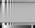
Log Frequency, Log F-Contrast (sine or bar) |
Sharpness, Color moiré, Detail lost to software noise reduction |
Rescharts Log Frequency, Log F-Contrast |
MTF is a check on the slanted-edge method; more direct but less accurate. |
Siemens star chart |
Sharpness |
Star chart |
Imatest Master only. May be created for printing by Test Charts or purchased from Image Engineering. |
Test images
These images were put online for testing Imatest API/EXE, but they are generally useful for testing Imatest. This is not a comprehensive list of charts, which can be found in the above table.
| Module |
Image file |
Description |
|
|
Webcam image of high and medium contrast custom charts created by Test Charts and printed on an Epson R2400 printer: these can have larger regions of interest (ROIs) than the ISO 12233 chart below. |
|
Webcam image of ISO 12233 chart. At this distance the available regions of interest are very small. |
|
|
Webcam image of the Kodak Q-14 grayscale and GretagMacbeth ColorChecker. |
|
|
Image of the Stouffer T4110 transmission test chart taken with the Canon Powershot G2. Excellent dynamic range measurement. |
|
Webcam image of the Kodak Q-14 grayscale and GretagMacbeth ColorChecker. |
|
12-patch OECF chart (for API and Imatest Master only ). Available from Applied Image. |
|
Image of Kodak Q-14 chart with "black hole" cavity for measuring veiling glare (susceptibility to lens flare) |
|
|
Webcam image of distortion grid. |
|
|
Image of nearly uniformly illuminated surface taken with the Canon 10-22mm lens on the EOS-20D, f/4.5, 22mm, ISO 1600. |
|
|
Image Log-Frequency-Contrast chart (cropped), acquired by the EOS-20D camera, 24-70mm f/2.8L lens set at 42mm, f/5.6, ISO 100. Can also be used with Log Frequency. |
Algorithms
| Module |
Algorithm link |
Brief description |
| Stepchart |
www.imatest.com/docs/q13.com#Algorithm |
|
|
|
Slanted-edge MTF measurement. The calculation is derived from ISO-12233. The average edge is calculated using a 4x oversampling binning algorithm. MTF is the Fourier transform of the derivative of the differentiated edge (the average line spread function (LSF)). The Imatest algorithm is more immune to noise and lens distortion than the standard ISO algorithm, which can be selected in a checkbox if desired. |
FAQ
Frequently Asked Questions
Frequently Asked Questions about Imatest™
How is Imatest pronounced?
Imatest is pronounced like a contraction of "Image" and "test." It is not pronounced like "I'm a test." But we'd rather hear it mispronounced than not pronounced at all.
How do I get started?
Begin by reading Image quality factors and the Tour pages Then download and install the evaluation version. The evaluation version allows up to 20 runs of individual modules, enough to show you what Imatest can do. We strongly encourage you to try before you buy. After you purchase Imatest, you'll need to register it to upgrade to the full version. Registration is self-explanatory, especially on computers connected to the Internet. If your computer is offline or behind a strong firewall, you'll need to follow the offline registration instructions.
The essential Imatest workflow is (1) photograph a test chart, (2) save it in a standard file format (TIF, high quality JPG, PNG, etc.), then (3) open it for analysis in the appropriate Imatest module. All instructions are available online. Imatest Master can also analyze Bayer RAW files.
Which version should I buy?
If you are a photographer planning to test your cameras and lenses, Imatest Studio should meet your needs. If you are an imaging system developer or if you are involved in intensive testing, you will appreciate the extra features of industrial-strength Imatest Master, outlined in Version comparisons and on the Purchase page. If your needs grow you can always upgrade from Studio to Master.
How do I purchase Imatest ?
Imatest is normally purchased with a credit card from our online store, which is linked from the Purchase page. Several alternative means of purchase are available, including wire transfer and custom Paypal invoice (faster and less expensive than a wire transver) that we can create on request. These are useful for custom orders (e.g., academic / educational / quantity discounts). If you have an inquiry, please contact
.
I purchased Imatest but didn't receive the confirmation email with the password. What should I do?
If you fail to receive the confirmation email, it may have been intercepted by a strong SPAM filter such as Spam Arrest, which requires that emails be sent from authorized domains or manually confirmed. If you have such a filter, please ensure that it allows emails from '@imatest.com.' You may be able to find the missing email in your SPAM mailbox. If you don't receive the email within about fifteen minutes, contact us.
Is there a CD version? Will I receive anything in the mail?
No. Imatest is only available as an Internet download. You will receive nothing in the mail. All Imatest documentation is available on the website. A CD is available on special request, but not recommended because Imatest is frequently updated, and you'll want to keep your installation up to date by downloading and installing the latest version. You are entitled to free upgrades for one year from the date of purchase. After a year you'll need to renew your subscription to install the latest updates.
How do I install Imatest on a computer that isn't connected to the Internet?
Download the current version of Imatest as well as the Imatest Library to a computer that is connected to the Internet. You may also want to download the PDF version of the documentation, though the website is usually more up-to-date and easier to navigate. Techniques for downloading individual web pages are given below. Copy the downloaded files to a USB memory device (you can burn a CD, but USB devices are handier) and transfer them to the offline computer. Install Imatest by double-clicking on the installation file, Imatest-version.exe. Then follow the offline registration instructions.
What test charts do I need? Are they included with Imatest?
Test charts are listed in the instruction pages for the individual modules (click on any of the links below), and they are summarized on the Cross-reference page. They are not currently supplied with Imatest, though you can print charts for SFR, Distortion, and Rescharts on high quality inkjet printers using the Test Charts module. Charts for measuring tonal and color response (using Stepchart, Colorcheck, and Multicharts) must be purchased; inkjet prints don't have accurate enough tonal response or sufficient color gamut.
- SFR For large charts (24 inches = 60 cm or wider) excellent results can be obtained with charts created by the Imatest Test Charts module and printed on a high quality inkjet printer. Several smaller charts can be combined on foam board. The SVG charts have several advantages over ISO charts: much less wasted area and lower contrast, which produces more accurate and consistent results.
- SFR For 13x19 inch (Super A3) or smaller charts, finer results can often be obtained with photographically-printed charts, which have better MTF (i.e., sharper edges). The QA-72 and QA-77 charts from Applied Image are excellent. Applied Image offers a discount on Imatest software purchased at the same time as their charts.
- Colorcheck uses the widely available 24-patch GretagMacbeth Colorchecker.
- Stepchart uses linear grayscale step charts such as the Kodak Q-13/Q-14 (reflective) or the Stouffer T4110 (transmissive). It also uses specialized charts (OECF, etc.) from Applied Image and others.
- Multicharts uses the the 24-patch GretagMacbeth Colorchecker, the ColorChecker SG, the IT8.7, the CMP DT 003, the QPCard 201, and several grayscale charts.
A detailed list of test charts, corresponding image quality factors, and Imatest modules is given in the Cross Reference.
What is Matlab? Do I need it to run Imatest?
Imatest is written in Matlab, a high level interpretive computer language designed for the efficient solution of scientific and engineering problems. It has particularly powerful graphics. Matlab source code requires Matlab to run. But Imatest has been compiled with the Matlab Compiler to run on any Windows computer. Compiled Matlab programs require the Matlab runtime library, which is installed along with Imatest. Installation is automatic on computers connected to the internet. Details can be found on the Imatest Installation page.
If you want to write your own analysis programs, consider one of the free Matlab clones. Well... almost clones. They're not as powerful and not fully compatible (and they don't have compilers), but the price is right. Octave and Scilab are the most recommended. Some image processing packages are also available, for example, Imlab.
When will a Macintosh version be available?
As much as we'd like to, we cannot make a commitment at this time. The new Matlab Compiler works under Mac OS X, but it's something of a bloatware monstrosity (requiring a 120 MB library download), and there are a number of additional devilish details to resolve. We have several high priority projects to tackle first (see Plans), but the Mac version is extremely important, especially for the educational market.
How often is Imatest updated?
Imatest is typically updated every week or two, except when we're traveling. It is updated whenever a feature is added or a bug is fixed. Minor updates are indicated incrementing x in version 2.n.x; major updates (usually new modules, such as Distortion or Starchart) are indicated incrementing n. Significant updates are announced on the main page. Full details of updates are posted in the Change log.
I purchased Imatest several months ago. How do I get the latest version?
You are entitled to free updates to Imatest for one year from the date of purchase. If you purchased Imatest more than a year ago, you should renew your license before downloading the latest version. You can download the latest version from the Download page. To install it, just double-click on the download file (Imatest-n.m.x.exe). You don't need to uninstall the previous version (though it may be advisable in rare instances of trouble). Versions are listed in the Change log. Full instructions are on the Installation page.
Imatest isn't working. What do I do?
Make sure you have the latest version. The primary causes of installation or registration failure are strong firewalls and lack of administrator privelege (rare except in highly-secure networked systems). If the troubles persist, go to the Troubleshooting page, which explains how to collect the information needed to identify the problem. E-mail it to Imatest support.
How can I download Imatest documentation for offline viewing?
There are two ways: you can download a PDF document that contains the entire website (over 8 MB) or you can download individual pages. The PDF documentation (on www.imatest.com/docs/Imatest_Documentation.pdf) may be a little out of date— it's updated infrequently. It's also long (215 pages at last count) and difficult to navigate. Downloading the current (individual) pages is recommended where feasible.
Create a convenient folder for storing the website. Then open a web browser and go to a page you want to save. You may want to click on , as described below.
- From Internet Explorer, click on File, Save As..., then save the web page (complete) in the folder you created. A subfolder will be created for the images.
- From Mozilla or Firefox, click on File, Save Page As..., then save the web page (complete) in the folder you created. A subfolder will be created for the images.
- As an alternative, you can create a PDF document by printing to PDFCreator (see the section below for optimizing the format). PDFCreator is an incredibly useful free open source program. Strongly recommended. Windows Vista users will need CutePDF Writer.
With this technique you can download the entire website in minutes.
How can I get the good printouts of Imatest documentation?
Click on in the box on the upper-right of the page. This loads a version of the page that prints correctly because the header and sidebar are omitted. Click the Back button to return to the regular page and restore normal navigation.
On most browsers, images tend to print too large with the default settings.
On Internet explorer version 6 or lower the image size cannot be reduced, hence IE 6 or lower is not recommended for printing web pages. However, IE 7 may have this capability.
On Mozilla/Firefox, click File, Print Preview, then set the Scale box at the top of the page to 80%. (The default is Shrink To Fit.) You can also click Page Setup and set Print Background (colors & images) and Margins &Header/Footer as desired. Then click OK. The print preview image may look a little rough (links are oversized), but the page should print nicely.
The Display resolution setting (accessible in Firefox by clicking Tools, Options..., Fonts & Colors, or in Mozilla by clicking Edit, Preferences, Appearance, Fonts) has no effect on image size.
The Opera browser produces excellent printouts with appropriately-sized images using the Print options settings shown on the right. Downloading and installing Opera is simple and straightforward. |
 |
What are the terms of the Imatest license?
The Imatest (Studio and Master) license allows an individual user to install and use the software on (A) a maximum of three computers (for example, home, laptop, and office) used exclusively by a single individual, or (B) a single workstation used nonsimultaneously by multiple people, but not both. It is not a concurrent use license. If more than one person uses Imatest on more than one computer, you should purchase additional licenses.
License holders are encouraged to publish test results in printed publications, websites, and discussion forums, provided they include links to www.imatest.com. You may not use Imatest for advertising or product promotion without explicit permission from Imatest LLC. Contact us if you have questions. The full text of the license can be found here.
What are those green boxes all about?
Green is for geeks. Do you get excited by a good equation? Were you passionate about your college math classes? Then you're probably a math geek— a member of a maligned and misunderstood but highly elite fellowship. The text in green is for you. You'll also enjoy the numerous links to the ultimate math geek resource: MathWorld, hosted by Wolfram Research. If you're normal or mathematically challenged, you may skip these sections. You'll never know what you missed.
What are Imatest's plans? Without giving too much away,
- Continued development of EXE and DLL versions of several modules for automated testing. Imatest API/EXE is now available.
- New modules for measuring MTF that take advantage of the SVG test charts to achieve higher levels of automation— especially automated detection of regions of interest (ROIs). 3rd Quarter 2008.
Please write us to let us know your needs. Our priorities are strongly influenced our customers.
Imatest is committed to providing individual photographers, researchers, developers, and manufacturers with comprehensive solutions for measuring digital image quality. Whether you are an individual photographer with lenses to test or a manufacturer of imaging chips and modules, Imatest has something for you.
Version comparisons
Differences between versions. Which is right for you?
Imatest versions
Imatest is available in two versions.
- Imatest Studio, with everything individual photographers need to test their cameras, lenses, and printers.
- Imatest Master, the full-featured industrial-strength version for professionals and imaging system developers.
Comparision between versions
| SFR |
Studio |
Master |
| Edge and MTF (SFR) plot |
 |
|
| Chromatic aberration plot |
|
|
| Batch runs (multiple input files) |
6 max. |
|
| SFR Any Angle: Calculate MTF for any edge angle. |
|
|
| Display edge and MTF for R, B, and B channels, in addition to Y (luminance) channel |
|
|
| Colorcheck |
Studio |
Master |
| Tonal response and noise analyses for B&W patches |
|
|
| L*a*b* color error and Color analysis |
|
|
| Batch runs (multiple input files) |
|
|
| User-supplied reference files |
|
|
| Noise analysis for R, G, B, C, M, and Y patches; noise spectrum |
|
|
| Multicharts |
Studio |
Master |
| Interactive analysis of tones and colors in the 24-patch GretagMacbeth Colorchecker and IT-8.7 charts |
|
|
| Analysis of the GretagMacbeth ColorChecker SG |
|
|
| User-supplied reference files |
|
|
| Special charts: analyze patterns of squares arranged on a circle as well as the Applied Image and ISO charts also analyzed by Stepchart for Imatest Master . |
|
|
| Stepchart |
Studio |
Master |
| Tonal response, noise, and dynamic range analysis |
|
|
| Batch runs (multiple input files) |
|
|
| Tonal response for separate R, G, B, Y channels (figure 3) |
|
|
| Chart density (reference) values can be read from a file. |
|
|
| Analyzes the Applied Image QA-61 (ISO-16067-1), QA-62, ST-51 (EIA grayscale), and ST-52 (ISO-14524) charts, and the ISO-15739 (Noise) chart. |
|
|
| Rescharts |
Studio |
Master |
| SFR Edge and MTF plots, Chromatic aberration plots. See SFR (above) for more details. |
|
|
| Log Frequency MTF plot |
|
|
| Log Frequency Color moiré plot |
|
|
| Log Frequency-Contrast (MTF, normalized contrast, etc.); shows effects of noise reduction |
|
|
| Light Falloff |
Studio |
Master |
| Light falloff (luminance channel) displayed in normalized pixel levels and f-stops |
|
|
| Batch runs (multiple input files) |
|
|
| Light falloff for R, G, and B channels |
|
|
| Display dead and hot pixels |
|
|
| Histogams for R, G, and B channels |
|
|
| Display color shading (color nonunformity of sensor) |
|
|
| Noise detail |
|
|
| Test Charts |
Studio |
Master |
| SFR Quadrants, SFR rectangles, Grid (for Distortion) |
|
|
| Star, Log-frequency contrast/gradient, Zone plate |
|
|
| Create Scalable Vector Graphics (SVG) charts. |
|
|
| Distortion |
Studio |
Master |
| Calculate distortion for 3rd and 5th order polynomial and tan/arctan approximations. |
|
|
| Batch runs (multiple input files) |
|
|
| Calculate lens decentering |
|
|
| Intersection point plot |
|
|
| Corrected image display |
|
|
| MTF Compare |
Studio |
Master |
| Allows MTF results calculated in SFR and saved in CSV files to be compared for a wide variety of cameras, lenses, and imaging systems. |
|
|
| Print Test |
Studio |
Master |
| Print tonal response and gamut in La*b* and xyY spaces |
|
|
| Print gamut in HSL representation |
|
|
Glossary
Aliasing
|
|
Low frequency artifacts, sometimes quite disturbing, that appear when signal energy above the Nyquist frequency
reaches the digital sensor. Color aliasing in Bayer sensors can be
particularly troublesome. "Moire fringing" is a type of aliasing. |
| Aperture |
|
The circular
opening at
the center of a lens that admits light. Generally specified by the
f-stop,
which is the focal length divided by the aperture diameter. A large
aperture
corresponds to a small f-stop. This can confuse beginners. |
Bayer sensor
|
|
The
sensor pattern used in most digital cameras, where alternate rows of
pixels are sensitive to RGRGRG and GBGBGB light. (R = Red; G = Green; B
= Blue.) To be usable, the sensor output must be converted into a standard file
format (for example, JPEG, TIFF, or PNG), where each pixel represents
all three colors, by a RAW converter (in the camera or computer), which
performs a "demosaicing" function. The quality of RAW converters
varies: separate converter programs run in computers can provide finer
results than the converters built into cameras. That is one of the
reasons that RAW format is recommended when the highest image quality
is required. Starting with version 2.7, Imatest Master can analyze Bayer raw files.
In Foveon sensors (used in Sigma cameras), each pixel site is sensitive
to all three colors. Foveon sensors are less susceptible to color
aliasing than Bayer sensors; they can tolerate greater response above Nyquist with fewer ill effects. |
Chromatic
aberration
(CA) |
|
A lens
characteristic that
causes different colors to focus at different locations. There are two
types: longitudinal, where different colors to focus on different
planes,
and lateral, where the lens focal length, and hence magnification, is
different
for different colors. Lateral CA is the cause of a highly visible
effect
known as color fringing. It is worst in extreme wide angle, telephoto,
and zoom lenses. Imatest SFR
measures lateral CA (color fringing). Measurements are strongly affected by demosaicing; accurate measurements for lenses must be done on raw files, which can be done starting with Imatest Master 2.7. See Chromatic
aberration and Eliminating
color fringing. |
Cycles,
Line Pairs,
Line Width |
|
A Cycle is the period a complete repetition of a signal. It is used for frequency measurement. A Cycle is equivalent to a Line Pair. Sometimes Line Widths are used for historical reasons. One Line Pair = 2 Line Widths. "Lines" should be avoided when describing spatial frequency because it is ambiguous. It usually means Line Widths, but sometimes it is used (carelessly) for line pairs. |
| Demosaicing |
|
The process of converting RAW files, which are the unprocessed output of digital camera image sensors, into usable file formats (TIFF,
JPEG, etc.) where each pixel has information for all three colors (Red, Green, and Blue). For Bayer sensors, each RAW pixel represents a single color in RGRGRG, GBGBGB,
... sequence. Although demosaicing is the primary function of RAW converters, they perform additional functions, including adding a gamma curve and often an additional tonal response curve,
reducing noise and sharpening the image. |
Density
(Optical density)
.
. |
|
The
amount of light reflected or transmitted by a given media, expressed on
a logarithmic (base 10) scale. For reflective media (such as
photographic
or inkjet prints), density = –log10(reflected light/incident
light). For transmissive media (such as film), density = –log10(transmitted
light/incident light).The higher the density, the less light is
transmitted
or reflected. Perfect (100%) transmission or reflection corresponds to
a density of 0; 10% corresponds to a density
of 1; 1% corresponds to a density of 2, etc. Useful equations:
1 f-stop (1 EV) = 0.301 density units; 1 density unit = 3.32 f-stops (EV).
When an object is photographed, Log10 Exposure = –density + k. (Constant k is generally ignored.) |
Dynamic
range
|
|
The range of exposure (usually measured in
f-stops) over which a camera responds. Also called exposure range. Practical dynamic range is
limited by noise, which tends to be worst in the darkest regions.
Dynamic range can be specified as total range over which noise remains under a specified level— the lower the
level, the higher the image quality. Dynamic range is measured by Stepchart, using transmission
step charts. |
| Exposure |
|
The definition depends on the context.
1. In Imatest results, "exposure" is the amount of light reaching a region of the sensor. Imatest plots often use Log Exposure (where Log is log10 in this context) because the human eye's response is roughly logarithmic. For test chart images, Log exposure is proportional to −optical density.
2. In other contexts "exposure" may refer to the combination of exposure time and lens aperture, which can be expressed quantitatively in EV. |
| Exposure value (EV) |
|
A
measure of exposure (definition 2), where a change of one EV corresponds to doubling or halving
the total light reaching the image plane. Often synonymous with f-stop (in the context of exposure change). By definition, 0 EV is a 1
second exposure at f/1.0. EV = log2(N2/t) where N = f-stop and t = exposure time. Note that EV is based on log2 while density is based on log10.
(Here in Boulder, Colorado, residents perfer to use "enlightenment", which is based on natural logarithms (loge, where e = 2.71828...). Boulderites strongly prefer products labeled "natural", "organic", or "green", or prefixed "eco-", "enviro-", etc. 1 Enlightenment Unit (€) = 0.4343 Density units = 1.443 EV.) |
f-stop
. |
|
A
measure of the a lens's
aperture (the circular opening that admits light). A a change of "one f-stop" implies doubling or halving
the exposure. This is the synonymous with a change of 1 EV.
F-stop = focal length / aperture diameter. The notation, "f/8," implies
(aperture diameter = ) focal length/8. The larger the f-stop number,
the
smaller the aperture. F-stops are typically labeled in the following
sequence,
where the admitted light decreases by half for each stop: 1, 1.4, 2,
2.8, 4,
5.6, 8, 11, 16, 22, 32, 45, 64, ... Each f-stop is the previous f-stop
multiplied by the square root of 2. |
Gamma |
|
Exponent
that relates pixel levels in image files to the brightness of the monitor
or
print. Most familiar from displays, where luminance = pixel levelgamma.
A camera (or film + scanner) encodes the image so that pixel level =
brightness(camera
gamma) (approximately). Imatest reports
camera gamma.
Gamma is equivalent to contrast. This can be observed in traditional film curves, which are
displayed
on logarithmic scales (typically, density (log10(absorbed
light)
vs. log10(exposure)). Gamma is the average slope of this
curve
(excluding the "toe" and "shoulder" regions near the ends of the
curve),
i.e., the contrast. See Kodak's
definition in Sensitometric
and Image-Structure Data. For more detail, see the
descriptions
of gamma in Using Imatest SFR
and Monitor
calibration.
Confusion
factor: Digital cameras output may
not follow an exact gamma (exponential) curve: A tone reproduction curve
(usually an "S" curve) may be superposed on the gamma curve to boost
visual contrast without sacrificing dynamic range. Such curves boost
contrast in middle tones while reducing it in
highlights
and shadows. Tone reproduction curves may also be adaptive:
camera gamma may be increased for low contrast scenes and decreased for
contrasty scenes. (Hewlett-Packard advertises this technology.) This can affect the accuracy of SFR measurements. But
it's not a bad idea for image making: it's quite similar to the
development
adjustments (N-1, N, N+1, etc.) Ansel Adams used in his zone
system. |
Image editor
Image viewer |
|
An image editor is a program for editing and printing images. The most famous is Adobe Photoshop, but Picture Window Pro is an excellent choice for photographers (though it doesn't have all the graphic arts features of Photoshop). If you don't have one, get Irafanview, which is more of an image viewer— a program for reading, writing, and viewing images. Irafnview can read and write images in almost any known format, and it also includes simple editing capabilities. Image editors contain more sophisticated functions, like masks, curves, and histograms. |
| ISO speed |
|
The
sensitivity of a camera to light. Sometimes called Exposure Index. The higher the ISO speed, the less
exposure is required to capture an image. In digital cameras ISO speed
is adjusted by amplifying the signal from the image sensor prior to
digitizing it (A-D conversion). This increases noise along with the image signal. ISO speed was called ASA speed in the old days. See Kodak Application Note MTD/PS-0234: ISO Measurement and Opsci Application Notes. |
| MTF |
|
Modulation
Transfer Function.
Another name for Spatial Frequency Response (SFR). Indicates the
contrast
of a pattern at a given spatial frequency relative to very low spatial
frequencies. See Sharpness and Understanding
image sharpness and MTF curves. |
| MTF50 |
|
The spatial frequency where image contrast is half (50%) that of low frequencies. MTF50 is an excellent measure of perceived image sharpness because detail is diminished but still visible, and because it is in the region where the response of most cameras is declining most rapidly. It is especially valuable for comparing the sharpness of different cameras. See Sharpness and Understanding image sharpness and MTF curves. |
| MTF50P |
|
The spatial frequency where image contrast is half (50%) the peak value. MTF50P is the same as MTF50 in imaging systems with little to moderate sharpening, but is lower for systems with heavy sharpening, which have a peak in their MTF response. MTF50P is increased less than MTF in strongly oversharpened cameras; it may be a better measurement of perceived image sharpness than MTF50 in such cases. See Sharpness and Understanding image sharpness and MTF curves. |
Noise
|
|
Random
variations of image luminance arising from grain in film or electronic
perturbations in digital sensors. Digital sensors suffer from a variety
of noise mechanisms,
for example, the number of photons reaching an individual pixel or resistive (Johnson) noise. Noise
is a major factor that limits image quality. In digital sensors it
tends to have the greatest impact in dark regions. It is worst with small pixels (under 3 microns).
Noise is measured as an RMS value (root mean square; an indication of noise power, equivalent to standard deviation, sigma).
It is usually expressed in volts, millivolts, or pixel levels (in a
digital file). In Stepchart and Colorcheck, noise is converted
to relative luminance units (f-stops), which may provide a more meaningful indication of its visual impact.
Software noise reduction, used to reduce the visual impact of noise, is a form of lowpass filtering (smoothing) applied to portions of the image that to not contain contrasty features (edges, etc.). It can cause a loss of low contrast detail at high spatial frequencies. The Log F-Contrast module was designed to measure this loss.
The visual impact of noise is also affected by the size of the image—
the larger the image (the greater the magnification), the more
important noise becomes. Since noise tends to be most visible at medium
spatial (actually angular) frequencies where the eye's Contrast Sensitivity Function is large, the noise spectrum has some importance (though it
is difficult to interpret). To learn more, go to Noise in photographic images. |
.
.
Nyquist
frequency |
|
The
highest
spatial frequency where a digital sensor can capture real information.
Nyquist frequency
fN = 1/(2 * pixel
spacing). Any information above fN that reaches the
sensor
is aliased to lower
frequencies,
creating potentially disturbing Moire patterns. Aliasing can be
particularly
objectionable in Bayer sensors in digital cameras, where it appears as
color bands. The ideal lens/sensor system would have MTF = 1 below
Nyquist
and MTF = 0 above it. Unfortunately this is not achievable in optical
systems;
the design of anti-aliasing (lowpass) filters always involves a
tradeoff
that compromises sharpness.
A large MTF
response above
fN
can indicate potential problems with aliasing, but the visibility of
the
aliasing is much worse when it arises from the sensor (Moire patterns) than it is when it arises from sharpening
(jagged edges; not as bad). It is not easy to tell from MTF curves exactly which of these effects dominates. The
Nyquist sampling theorem and aliasing contains a complete exposition. |
Raw files
Raw conversion |
|
RAW files are the unprocessed output of digital camera image sensors, discussed in detail here. For Bayer
sensors, each RAW pixel represents a single color in RGRGRG, GBGBGB,
... sequence. To be converted into usable, standard file formats (TIFF,
JPEG, etc.), raw files must be run through a RAW converter
(demosaicing program). RAW converters perform additional functions:
they add the gamma curve and often an additional tonal response curve,
and they reduce noise and sharpen the image. This can interfere with
some of Imatest's measurements.
The best way to be sure an image file faithfully resembles the RAW
file— that it has no sharpening or noise reduction— is to read a RAW
file into Imatest, which uses Dave Coffin's dcraw to convert it to a standard format (TIFF or PPM).
Imatest documentation sometimes distinguishes between camera RAW files— camera manufacturer's proprietary formats, and Bayer RAW files— undemosaiced files that contain the same data as camera raw files, but are in standard easily-readable formats such as TIFF or PGM. Dcraw can convert camera RAW files into Bayer RAW files. Starting with version 2.7, several Imatest Master modules can measure camera RAW files directly. |
Resolution
|
|
The first thing to remember about resolution is that it has no unique definition. It can be defined in many ways, some of which can be quite misleading. (It is almost as abused as the word "holistic.") In a generic sense, resolution refers to any measurement of an imaging system's ability to resolve fine detail. For traditional film cameras, it usually refers to vanishing resolution— the
highest
spatial frequency where the pattern on a bar chart (usually the USAF
1951
chart) was visible. Since this tells you where detail
isn't,
it's not a very good indicator of perceived sharpness. The pixel per
inch
(PPI or DPI) rating of a scanner is often called its "resolution." This
can be highly misleading. For example, some inexpensive flatbed scanners
can't
come close to resolving the detail of decent film scanners with the
same
PPI rating; their lenses aren't up to the job. I prefer MTF50 (the spatial frequency where contrast falls to half its low frequency value) as a measure of resolution. For more on
resolution,
see Pixels,
Images,
and Files and Lens
testing (the old-fashioned way). |
| SFR |
|
Spatial Frequency Response. The response of a system to a pattern at a given spatial frequency, i.e., the contrast. SFR is measured relative to contrast at very low spatial frequencies. It is expressed as a fraction or percentage. Synonymous with MTF. See Sharpness and Understanding image sharpness and MTF curves. |
| Sharpening |
|
Signal processing applied to digital images to improve perceived image sharpness. It can be applied in the camera or in post-processing (image editing). Virtually all digital images benefit from some degree of sharpening, but images can be oversharpened, resulting in highly visible "halos" (overshoots) near edges. See Sharpening. |
Standardized
sharpening |
|
An algorithm used by Imatest that allows cameras with different amounts of sharpening to be compared fairly. With standardized sharpening, all cameras have a similar amount of overshoot (around 5%) near edges. Without it, built-in sharpening strongly affects test results, giving oversharpened cameras an unfair advantage. Results with standardized sharpening should not be used for comparing different lenses on the same camera. See Standardized sharpening. |
| Tone reproduction curve (TRC) |
|
A curve that describes a camera's response to light. Usually displayed as Density or Log pixel level vs. Log exposure. Often refers to an "S"-shaped curved applied on top of the gamma curve during Raw conversion. The purpose of such a TRC is to increase visible (midtone) contrast while maintaining detail in shadows and highlights. |
Customers and publications
A list of better-known customers and publications
Imatest partners
Imatest has a co-marketing agreement with Applied Image, a leading supplier of test charts for industry. You can receive a price break by purchasing Imatest along with an Applied Image chart.

Additional agents and resellers
Imatest customers
Imatest has been adopted by a wide range of industries that employ embedded digital imaging systems, including mobile imaging (camera phones), medical imaging, aerospace and machine vision, as well as publications/reviews, and academic, cultural, and research institutions. Here are some of Imatest's better-known customers.
Sites that use or describe Imatest
An ever-growing number of publications use Imatest for camera and lens reviews. Please contact us if you'd like us to add your site.
| Norman Koren's Google TechTalk, Image Quality Measurement: Real world challenges, is available online. For a clearer view of the image quality factors, download the the Presentation (PDF format) (2.8 MB). |
| The 12.8 megapixel Canon EOS 5D digital SLR is receiving a lot of attention for its superb quality at less than half the price of the EOS 1Ds Mark II. See Imatest results on Digitalcamerainfo.com | gnyman.com | Peter Facey |
| Volker Gilbert has written an excellent French language description of Imatest. (PDF version). René Bouillot has included a chapter on Imatest in his new book, La pratique du reflex numérique. |
| Sites using Imatest for reviews |
CNET uses Imatest for testing digital cameras.
Digital Photographer (UK) is the first English language print magazine to feature Imatest reviews.
Digitalcamerainfo.com, from the creators of Camcorderinfo.com, has in-depth reviews that take full advantage of Imatest.
PhotoReview.com.au, from the publishers of PhotoReview Australia, uses Imatest in its reviews of popular digital cameras.
Imaging-resource.com also takes full advantage of Imatest for its reviews. See, for example, the Canon EOS 1Ds Mark II.
PC Magazine is using Imatest for camera reviews, starting in Oct. 2008.
Photodo.com, a site with a distinguished history of testing lenses, is now using Imatest for its lens tests.
Photozone.de (Klaus Schroiff), uses Imatest for lens reviews. example: the Canon EF-S 10-22mm ultrawide.
D-Spot (Hebrew language) uses Imatest in its reviews, starting with the Kodak SLR/n (pages 4 and 5) and the Fujifilm S3 Pro.
Gordon Laing's Cameralabs.com site is expanding its use of Imatest in camera and lens reviews.
Miljenko Devcic has a number of interesting lens tests and comparisons.
Optyczne.pl (Polish language) |
Read Norman Koren's interview with Steve Kapsinow, March 2, 2006. Steve is an editor of Graphics.com.
David Pogue notices! He published excerpts of a letter about Imatest's SQF measurement in Last Notes on the Megapixel Myth. |
Glosario en Espanol
Imatest Glosario
Par Pablo Ruiz Garcia
Aliasing.
Elementos de baja frecuencia, a veces muy molestos, que aparecen cuando la energía de la señal alcanza al sensor digital por encima de la frecuencia Nyquist. El efecto de flecos moire son un tipo de alilasing.
Aberración cromática.
Es una característica de la lente que provoca que las distintas longitudes de onda formen foco en distintos puntos. Existen dos tipos; longitudinal, donde los diferentes colores forman su foco en planos distintos. Y, lateral, donde la longitud focal de la lente, por lo tanto la ampliación, es diferente para cada color. La aberración cromática lateral causa un efecto muy visible, un borde irregular de color, conocido color frimgering. (nosotros hemos medido la aberración cromática lateral)
Ciclos, pares de línea, ancho de línea.
Un ciclo es un periodo completo de repetición de una señal. Es usado para medir la frecuencia. Un ciclo es equivalente a un “par de líneas”. A veces, por razones históricas, se emplea “ancho de línea” –un par de líneas es igual a dos anchos de línea-. El término “líneas”, a secas, debe ser evitado cuando se describe frecuencia espacial, porque es intrínsecamente ambiguo. Normalmente significa “ancho de línea”, y a veces es utilizado, sin cuidado, como “par de líneas”.
Rango dinámico
Es el rango de exposición, normalmente medido en f-stops, dentro del cual un equipo puede producir una respuesta tonal. En la práctica, el rango dinámico esta limitado por el ruido, que tiende a ser peor en las zonas oscuras. El rango dinámico puede ser definido como el rango total sobre el cual el ruido permanece bajo unos niveles aceptables. Cuanto menor es este nivel, mejor es la calidad de la imagen.
f-stop .
Es una medida de la apertura de la lente. Un cambio en “un f-stop” implica doblar o dividir por la mitad la exposición. Esto es sinónimo de un cambio en 1 EV.
f-stop = distancia focal /el diámetro de la apertura. El número “f/8” significa distancia focal /8. Cuanto mayor es el número f-stop, menor es la apertura.
También se aplica como medida del rango dinámico de una imagen. En este caso los f-stop hacen referencia a la capacidad de la imagen de diferenciar tonos desde el blanco hasta el negro. Cada nivel de f-stop representa un aumento en la densidad de la imagen de 0,3.
Gamma
Es un dato que relaciona niveles de píxeles, en la imagen, con el brillo del monitor o la copia. En los monitores encontramos que la luminancia = nivel de píxelgamma. Mientras que en una cámara o un escáner el nivel de píxel = brillogamma.
Gamma es equivalente a contraste. Esto se observa en las curvas de reproducción tonal en fotografía convencional que muestran el contraste como una escala logarítmica. Gamma es la pendiente media de esa curva.
Las salidas de los equipos digitales pueden no seguir exactamente la curva de gamma exponencial. Una curva de reproducción tonal (normalmente una curva “S”) puede ser superpuesta en la curva de gamma para incrementar el contraste visual sin perjudicar al rango dinámico. Este tipo de curvas incrementan el contraste en los tonos medios mientras que lo reducen en las altas luces y las sombras. La curva de reproducción tonal también puede ser adaptada: la gamma se puede incrementar para escenas de bajo contraste, o reducir para imágenes muy contrastadas Es similar a los ajustes de revelado (N-1, N, N+1, etc.) que Ansel Adams usó en su sistema de zonas.
MTF
Función de transferencia de modulación (Modulation Transfer Function). Otro nombre es, respuesta de frecuencia espacial (Spatial Frequency Response, SFR). Indica el contraste de un patrón en una frecuencia espacial dada, generalmente en relación con frecuencias espaciales muy bajas.
MTF50
Es la frecuencia espacial donde el contraste de una imagen es la mitad (50%) que el contraste presente a bajas frecuencias. MTF50 es una medida excelente para percibir la nitidez porque el detalle disminuye pero todavía es visible, y porque está en la región donde la respuesta de la mayoría de los equipos digitales decae más rápidamente. Es muy válido para comparar la nitidez de distintos equipos.
Ruido
Son variaciones aleatorias de la luminancia de una imagen provocado por el grano en una película, o perturbaciones electrónicas en un sensor digital. Estos últimos sufren de una gran variedad de mecanismos que producen ruido, por ejemplo el número de fotones que alcanzan un mismo píxel. El ruido es el mayor limite a la calidad de la imagen digital. En los sensores digitales suele tener un mayor efecto en las zonas de sombras.
El impacto visual del ruido viene determinado por el tamaño de la imagen –cuanto mayor es la imagen, mayor es el efecto del ruido-. Éste tiende a ser más visible a bajas frecuencias espaciales, por lo tanto el espectro de ruido tiene una gran importancia.
Frecuencia Nyquist
Es la mayor frecuencia espacial donde un sensor digital puede obtener información real. Cualquier información por encima de este nivel que alcance el sensor es aliased –imitado, copiado, clonado, etc.- de información en las bajas frecuencias, creando unos patrones tipo moire bastante molestos. Aliasing puede ser particularmente desagradable en los sensores Bayer de los equipos digitales, donde aparece como bandas de color.
Un alta respuesta de la MTF por encima de la frecuencia Nyquist indica grandes problemas de aliasing. El efecto visible es peor cuando el aliasing parte desde el sensor, es entonces cuando se presenta en el enfoque. No es fácil concluir en las curvas de MTF cual de estos efectos es el dominante.
Conversión de ficheros RAW
Los archivos RAW son salidas sin procesar desde los sensores de las cámaras digitales. Para un sensor Bayer , cada píxel representa un solo color en una secuencia, RGRGRG, GBGBGB... Para convertirlo en ficheros manejables los ficheros RAW deben ser tratados con un programa de conversión. Estos programas realizan además otro tipo de acciones, añaden la curva de gamma, y muchas veces una mejora en la respuesta tonal, reducen ruido, y enfocan la imagen.
Resolución
La primero que se debe decir de la resolución es que no tiene una única definición. Se puede expresar de muchas maneras, algunas pueden ser erróneas. En términos generales resolución hace referencia a cualquier medida de un sistema digital que exprese su capacidad de resolver detalles finos. En fotografía convencional, con película, se refiere como “resolución de desvanecimiento” –se mide la mayor frecuencia espacial donde es visible un patrón de una carta de barras (normalmente la carta USAF 1951)-. Este método te dice donde no se ve un detalle, por lo tanto no parece muy buen indicador para percibir el enfoque.
El ratio de píxel por pulgada de un escáner es siempre llamado resolución. Esto puede ser muy erróneo. Por ejemplo, escáneres baratos de sobre mesa pueden llegar a tener un poder de resolución –expresado en el ratio de píxeles por pulgada-, tan grande como los escáneres buenos de películas. Un método que parece más eficaz para obtener datos fiables de la resolución real es el que nos aporta el MTF50.
Troubleshooting
What to do when Imatest doesn't work
Version
Be sure you have the current version. It may contain fixes for bugs from earlier versions.
The version number appears in the bar at the top of the Imatest main window. If it's not the same as the latest version in the Change Log, you should download, install, and run the latest version.
| |
To run Imatest in Windows Vista,
you'll need version 2.3.3 or later. |
Installation
Update installations do not normally require an uninstall of the previous
version, but if you encounter difficulties you may want
to uninstall and reinstall Imatest. The Uninstaller is accessable from the Start menu
(Start, All programs, Imatest, Uninstall) or from the Add or Remove Programs function of the Control Panel. It
gives you the option of keeping or removing the Matlab runtime library
archive,
Imatest-lib.exe. (Keep is the default;
you have to check the box to remove it.) Keeping it speeds up reinstallation.
Remove it only if you don't plan to reinstall Imatest or if you have good reason to suspect it may be corrupted (a rare occurrence). Click here for full installation instructions.
Problems during installation
Installation or registration can fail if
- You don't have administrator priveleges on your computer.
- Your computer is behind a strong corporate firewall.
This message sometimes appears in systems that have strong firewalls. It can usually be corrected by making sure the Matlab runtime library, Imatest-lib.exe, available from the Download page, is in the same folder as the Imatest installation file. You may need to temporarily disable your firewall and manually download the library file. |
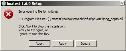 |
If you have receive an indication of a "DNS error" (very rare), try clicking Start, Run... Enter ipconfig /flushdns in the Open... box, then click OK.
Problems following installation
The most common installation problem is a failure of the Matlab runtime library, Imatest-lib.exe, to download or install properly. This results in an error message of the form,
"The procedure entry point ... could not be
located in the dynamic link library ... .dll."
If you get such a message, check to see if file Imatest-lib.exe has been downloaded correctly. Also, check the status of your firewall. Strong firewalls have caused this problem.
- If it was downloaded automatically (during installation) there should be a copy in the Imatest installation folder (C:\Program files\Imatest in English language installations).
- If you downloaded it manually (usually required in systems with firewalls), there should be a copy in the same folder as the Imatest installer program, Imatest-x.x.exe.
Windows XP Explorer reports its size as 8,513 kB, but the tooltip that appears when you move the cursor over the file name reports its size as 8.31 MB (go figure). If the download failed, a smaller size may be reported.
If you fail to find Imatest-lib.exe or if you suspect that it was downloaded incorrectly, download it by right-clicking here or on any of the links in this section, then reinstall Imatest. Imatest-lib.exe is a self extracting zip file that places the Matlab runtime library in subfolder bin\win32 and toolbox\matlab of the Imatest installation folder. If problems persist, check to see that these folders are populated, then send e-mail to Imatest support with the text of the error message, if any, that appears in the DOS window.
Missing DLL files In rare instances, four DLL files, jpeg_depth.dll, dataread.dll, imjpg8.dll, and rjpg8c.dll, may be missing from subfolder toolbox\matlab\iofun\private\ of the Imatest installation folder. Because they are not included in Imatest-lib.exe they are installed using a different procedure, which fails in fewer than 1% of installations. If you get a message that indicates they may be missing, you should check for them in the subfolder and install them manually if they are absent.
- In Imatest 3.1 or later, the four files are installed to the Imatest installation folder as well as the subfolder. They can be copied to the subfolder ( \toolbox\matlab\iofun\private\; C:\Program Files\Imatest\toolbox\matlab\iofun\private\ in English language installations) if they are missing.
- For earlier versions you can download jpegdlls.zip and copy the contents to the subfolder.
Runtime errors
If Imatest does not run as expected, the DOS window that normally stays minimized may contain helpful information. You can open it by clicking on the Imatest DOS Window icon in the taskbar. Here are some potential problems.
- An Imatest run may fail if the image file path name contains non-Latin characters. We have seen such a failure with Chinese characters. The error message was
The error message caught was : Invalid file identifier.
- Imatest.ini, the file that contains settings stored when modules are run, may have gotten corrupted.
Imatest.ini (and also rescharts.ini, multicharts.ini, etc.) contain saved settings that speed up Imatest runs. Settings include regions of interest (ROIs), plot selections, plot scales, and calculation techniques. Sometimes a setting gets corrupted and causes Imatest to crash.
Ini files are text files structured so that section titles are enclosed within brackets ( [ ... ] ) and lines have the form name = value, e.g., nwid_save = 2601.
[section]
name1 = value1
name2 = value2
...
[next_section]
There are several things you can do if you suspect that an ini file has been corrupted.
- In the Imatest Main window (or in the Rescharts or Multicharts windows), click Settings, Reset defaults (all). This deletes imatest.ini, then recreates it with a few default values. The sections are repopulated when modules are run.
- Click Settings, View settings (ini file). This opens imatest.ini in a simple editor (Notepad) that you can edit (if you have any idea what to change), then save by pressing control-S. You can also copy the contents and paste it into an email to Imatest support, as described below.
- Click Settings, Edit/reset module(s) to open the INI file Editor/Debugger, shown below.
You can select a section to view or delete from the Section dropdown menu. To edit a line, select it in the large window, make the change in the edit window just above the large window, then press Enter. To delete the entire selection, press the Delete section contents button. When you are ready to save the changes press the Save button, which is grayed out until changes are made. If you with to cancel your changes, press either Reload ini file or Close.
|
If you cannot solve the problem, send an e-mail to Imatest support.
- Tell us your operating system.
- Attach imatest.ini, which may contain helpful information for diagnosing the problem.
You can open imatest.ini (or multicharts.ini or rescharts.ini) by clicking on Settings, View settings (ini file) in the Imatest, Multicharts, or Rescharts windows, then you can copy the contents from Notepad and paste them into your e-mail. The ini files are located in %AppData%\Imatest, where %AppData% is a DOS environment variable whose file name can be determined by entering the command, dir "%AppData%" in a DOS window.
(You don't need to know the actual location.)
- In installations prior to Imatest 2.3 (the first release compatible with Windows Vista), the full file name was C:\Program files\Imatest\imatest.ini. (or counterparts in non-English installations, for example, C:\Programme\Imatest\imatest.ini in Deutsch.) When a version of Imatest prior to 2.3 is replaced with a newer version the file is automatically copied to the new location. Problems may occur when the %AppData% folder name contains non-Latin characters. (We are looking into this. The best solution may be to delete the old imatest.ini or move it manually.)
- Send the text of the error message, if any, that appears in the DOS window. (See the box below for instructions on getting a screen dump from the DOS window.)
The DOS window
Imatest runs from a DOS window that normally stays minimized. When a run terminates unexpectedly or just stalls, the DOS window may contain useful debugging information. To get the DOS window contents,
Click on the Imatest icon in the taskbar (usually at the bottom of the screen) to bring up the DOS window.
Procedure 1: Copy and paste text (simple, but a little tricky)
- Right-click inside the DOS window, then click on Select All in the context menu.
- Alternately, you can click on the icon on the upper-left of the window, click on Edit, click on Mark, then drag the cursor to select the text to copy.
- Press Enter (or Return) on the keyboard. This is equivalent to Ctrl-C (Copy) in Windows (which doesn't work in the DOS window).
- Paste the text into your e-mail using a standard Windows Paste command (Ctrl-V or Edit, Paste).
- It's OK to delete obviously irrelevant text before you send the e-mail.
Procedure 2: Copy and paste screen dump image (complex but reliable)
- Click Alt-PrtSc or Alt-PrintScreen, depending on the keyboard.
- Paste the image (from the clipboard) into an image editor. In most image editors (for example, IrfanView, a great free utility ), click Edit, Paste or control-V.
- Save the image as a GIF or PNG file (much smaller than TIFF or BMP and clearer than JPEG).
- Attach the file to the e-mail (or include it inline).
|
For Imatest errors that shut down the DOS window (this has become rare),
-
Run Imatest from the Imatest folder (C:\Program files\Imatest in English
installations) by double-clicking Diagnostics (or diagnostics.bat).
This keeps the DOS window open after Imatest terminates so you can view
the error message.
-
E-mail the error message to Imatest support. Tell us your Imatest version and operating system.
Path conflicts when other versions of Matlab are installed
X The procedure entry point svDoubleSclarRemW could not be
located in the dynamic link library libmwservices.dll |
If a different version of Matlab from the one used for Imatest (6.5.1) has been installed on your system, there is a tiny chance that you may experience a path conflict that causes a similar error message— or Imatest may simply fail to run. This rarely happens because the batch file that initiates Imatest sets the path. Path issues and solutions are discussed in API/EXE instructions.
Bugs and all that
The following message appears several times in the DOS window when
you try to save data.
Function
'get_param' is not implemented in standalone mode.
This has no effect on the saved images, and it's rarely
visible since the DOS window remains in the background. Matlab has described the problem, to be fixed in a future release, here.
The Open files dialog box in some modules cannot be resized. This is a bug in Matlab
Release 13. (However SFR has a new Open files dialog box that can be resized. And multiple files can be selected.)
More documentation
Instructions for individual Imatest
modules can be found in the Imatest Documentation
page.
Contact
About Imatest, and how to reach us
Imatest™ contact information
| |
|
Address:Imatest LLC
2500 Broadway St.
Boulder, CO 80304 USA |
|
Phone Numbers
Colorado USA: 720-438-4644
Toll Free: 800-599-3154
Fax: 720-746-5992
|
For difficulties in registering or running Imatest, please check the Troubleshooting page before contacting us.
For general support questions, write
 .
Please let us know which Imatest version and operating system you are using. We recommend that you check to see if you are running the current version. If not, we recommend that you download and install it.
.
Please let us know which Imatest version and operating system you are using. We recommend that you check to see if you are running the current version. If not, we recommend that you download and install it. |
|
You can usually open your email client by clicking on one of the email links on the left. If it doesn't work, enter it manually. |
|
To purchase Imatest, go to the Purchase page, which lists purchase options.
For questions about sales, write
.
For questions about the Imatest program, algorithms, instructions, or website content, write Norman Koren,
 .
.
Imatest background
Imatest was founded in Boulder, Colorado in 2004 to develop software for testing digital camera image quality and lens sharpness using simple, widely-available targets. It has been adopted by a wide range of industries and academic/cultural institutions. It is a spinoff of the highly informative digital photography website, www.normankoren.com.
Norman Koren, the founder and president, has been involved with photography since 1964. He holds a AB in physics from Brown University and an MA in physics from Wayne State University. His previous career in magnetic recording technology has provided him with an outstanding background for image quality analysis. He has received seven U.S. patents.
In May 2005 Norman was on a panel on the future of cameras at the MIT Symposium on Computational Photography and Video. In January 2006 he delivered a paper on Imatest at the Electronic Imaging conference. He authored Appendix C, Video Acquisition Measurement Methods (pp. 91-125), of the Public Safety SoR (Statement of Requirements) volume II v 1.0 (6 MB download), released by SAFECOM, prepared by ITS (a division of NTIA, U.S. Department of Commerce). No credit is given, but details of many Imatest algorithms are included. |
 |
| |
Travel plans 2008
Norman will be in northern California (Monterey area) Aug. 22-Sept. 1 and in San Jose in mid-September: may have some time to visit customers. He can be reached on his mobile phone, 720-985-9610 or at 720-438-4644 will work when he's at the computer. |
|
Henry Koren, Chief Technology Officer, has worked for eight years in developing database driven e-commerce web applications. Henry is currently pursuing a degree in computer science and engineering at the University of California San Diego.

Randy Bockrath, Vice President for Business Development, joined us in March 2008. Randy brings 20 years of experience in software engineering, consulting services, and executive management to Imatest. He has served in senior management roles at many organizations, from early stage to Fortune 100 companies. He has international business experience, has helped raise $8M in venture capital funding, founded startups with revenue of more than $1M, led Angel Investment groups, and lectured in eCommerce strategy. Randy holds a Ph. D. in Business Administration from the University of Minnesota where he majored in Information and Decision Sciences.
Agents and resellers
Several agents and resellers are available.
Imatest Change Log
Imatest release history
Imatest™ change log (release notes)
To obtain the latest version of Imatest (for updates, new installations, and trial as well as and full versions) go to Imatest Download. Imatest license holders are entitled to free updates for one year from the date of purchase. After that you need to renew. If you license is not current, you can download and install the version that was current one year after the purchase date from http://www.imatest.com/packages/Imatest-Release.exe where Release can be found in the table below. Example: http://www.imatest.com/packages/Imatest-2.5.4.exe .
You rarely need to uninstall an existing version. If you suspect that your installation has been corrupted, try clicking Settings, Reset Defaults (in the Imatest main window) before reinstalling.
| Date |
Release |
Description |
| Jan. 8, 2009 |
3.3 |
The Batchview module has been released for viewing summary results of batch lens tests (for example sequences of images at different f-stops). Dynamic Range and SFRplus calculations have been made more rubust. Imatest Studio can now run batches of up to six files (for use with Batchview). |
| |
| Dec. 26, 2008 |
3.2.5 |
A Vectorscope (pattern used for adjusting video/cinema cameras) has been added to Multicharts, along with support for the DSC Labs ChromaDuMonde 28 test chart . Optional constraints have been added to the color matrix calculation. Reload buttons have been added to Multicharts and Rescharts. |
| Dec. 2, 2008 |
3.2.4 |
A new View/Rename Files utility has been added so that files can be renamed using EXIF data-- a big help when large amounts of data has been taken and file names direct from cameras make little sense. The Help buttons have been repaired. |
| Nov. 26, 2008 |
3.2.3 |
Color/brightness profile plots, similar to plots in Light Falloff, has been added to SFRplus. An Image display for examining details (individual color channels and exaggerated saturation) has also been added, and region detection is more robust. |
| Nov. 12, 2008 |
3.2.2 |
Many small improvements make SFRplus calculations more robust. The noise spectrum has been added to histogram figure. Weighting options have been added to the Multicharts Color matrix calculation: highlights can receive stronger weight. |
| Nov. 7, 2008 |
3.2.1 |
EXIF metadata can be read in greater detail from all image file formats with the addition of Phil Harvey's ExifTool, which must be downloaded and installed following instructions here. Noise readouts and histograms in SFR and SFRplus have been greatly improved. Wider regions (ROIs) are available in SFRplus for improved noise analysis. Many SFRplus bug fixes. |
| Oct. 30, 2008 |
3.2 |
The SFRplus module, which implements automated ROI selection using a special test chart available for purchase, has been added. It measures distortion and tonal response in addition to MTF and Lateral Chromatic Aberrationn. Color correction matrix calculations in Multicharts have been significantly improved (with better starting values). Dcraw now includes dcrawMS, which works with Vista. Rescharts can read and average multiple files. |
| August 3, 2008 |
3.1 |
Multiple files can be read and averaged (and saved) to facilitate measurements of fixed-pattern noise (in Stepchart, Colorcheck, and Light Falloff) and image stabilization effectiveness (SFR). Highly distorted regions of interest (ROIs) can be analyzed with Colorcheck and Stepchart. New ΔE measurement options have been added to the Light Falloff Color shading display. Evaluation versions can be set for Master (default) or Studio mode. The Light Falloff hot/dead pixel display can be set to all/selected/any channel for color images. Several of the SVG test charts have been redesigned to work better with upcoming automated test modules. A new editor for INI files has been added to facilitate troubleshooting when modules stop working: sections can be easily located and their contents can be quickly edited or removed. |
| June 28, 2008 |
3.0.1 |
You can enter a DOS command from the Settings dropdown menu in the Imatest main window. This can be useful for troubleshooting (finding path issues, etc.). In Rawview you can select which of the two green channels (G(R) or G(B) to display) and you can save the undemosaiced image as a half-sized RGB file (using the selected green channel). |
| June 17, 2008 |
3.0 |
Light and Pro have been renamed Studio and Master. There is a new price schedule. Colorcheck has an option for selecting patches using 24 squares (similar to Multicharts) instead of the (old) standard auto patch detection. This can be valuable for distorted chart images. Single color analysis in SFR is faster than the standard 4 color analysis and useful for filtered images where some channels may have invalid data. The x and y-spacing and aspect ratio of the grid pattern is displayed in the Distortion intersection plot (useful for analyzing scanner aspect ratio distortion). The secondary readout in the SFR MTF plot can be emphasized (enlarged, bold face). |
| |
| March 21, 2008 |
2.7.2 |
Dynamic Range can calculate dynamic ranges of individual color channels (R, G, and B, as well as Y) in Imatest Master. Star Chart allows the number of calculation radii to be selected (32 (fastest), 64, or 128). It was formerly 32; the default is now 64. There is an additional option for low frequency MTF normalization. Some issues with reading custom density charts into Stepchart and Multicharts have been resolved. |
| March 18, 2008 |
2.7.1 |
Distortion can now analyze square (checkerboard) patterns. A gamma plot has been added to Dynamic Range. Star Chart can now accommodate a chart with a smaller inner circle (ID 5% of OD). |
| March 16, 2008 |
2.7 |
The new Dynamic Range module calculates camera dynamic range from the CSV output of several differently-exposed Stepchart runs. The Imatest main window has been rearranged. A checkerboard pattern has been added to to Test Charts and Screen Patterns. Several new video pattern sizes (6x0x480, etc.) have been added to Test Charts. |
| |
| March 8, 2008 |
2.6.12 |
Screen Patterns now includes SMPTE color bars, slanted-edge grid patterns, and a simulated Colorchecker and stepcharts. R-G and B-G shift in pixels has been added to the Chromatic Aberration display. |
| March 2, 2008 |
2.6.11 |
Screen Patterns now includes patterns for Distortion and Monitor calibration and a Zone plate for camera testing. The CSV and XML output of SFR now includes results at standard frequencies of (0.05, 0.1, 0.15, ... ) Cycles/pixel. |
| Feb. 24, 2008 |
2.6.10 |
The Screen Patterns module generates monitor test patterns for Light Falloff and SFR. A 4th order polynomial fit to Light Falloff is available in Imatest Master. Options & Settings has been divided into two windows (I and II) to accommodate more options. A new option for naming SFR output files is available. |
| Feb. 20, 2008 |
2.6.9 |
Chromatic Aberration display has been enhanced to include a thumbnail showing the ROI as well as R-G and B-G spacings that can be used for correcting CA (especially valuable with RAW images prior to demosaicing). |
| Feb. 15, 2008 |
2.6.8 |
CIEDE2000 color difference formulas have been added to Colorcheck and Multicharts. CIEDE2000 has replaced CMC measurements in some displays, but CMC measurements are available in the CSV output files. |
| Feb. 13, 2008 |
2.6.7 |
You can now choose between display of the cropped edge or entire edge in the SFR Edge & MTF plot. The entire edge is of interest for flare studies. A spot detection display has been added to Light Falloff for Imatest Master . |
| Feb. 7, 2008 |
2.6.6 |
SFR can now display spatial frequency in LP/PH (Line Pairs per Picture Height) in addition to LW/PH. This makes it easier to compare results with Dpreview.com's new lens reviews . The mapping between color and Bayer RAW channel can now be selected. This will affect some displays. |
| Feb. 4, 2008 |
2.6.5 |
The Rawview utility (next to dcraw) in the Imatest main window allows Bayer Raw files to be previewed and colors to be associated with pixel position. Bugs in calculating RAW Chromatic aberration were fixed. |
| Feb. 3, 2008 |
2.6.4 |
A GUI (graphic user interface) for dcraw, which can can demosaic RAW images or convert them into Bayer RAW format, can be called from the Imatest main window. In Imatest Master, SFR, Rescharts, and Stepchart can now analyze Bayer RAW files. Support for other modules will be gradually added; feedback appreciated. |
| Jan. 28, 2008 |
2.6.3 |
A new summary CSV output file (with a name of the form, filename_Y_sfrbatch.csv) is produced for multiple-ROI SFR batch runs. This file is particularly convenient for generating Excel plots of the type shown below, next to 2.6.1. |
| Jan. 18, 2008 |
2.6.2 |
Options & Settings (in Imatest main window) now offers options to shrink input files for Distortion and Light Falloff 1/2x to prevent memory overflow if they are over 40 or 80 MB (m x n x colors) and also to fix the order that batch files run (which may be different for different operating systems). Raw files can now be converted to Bayer raw (undemosaiced) TIFF files, and also work better in batch runs. |
| Jan. 8, 2008 |
2.6.1 |
 The SFR and SFR multi-ROI CSV output files have been enhanced to work better with high volume testing. A new summary block in the multi-ROI CSV file can be conveniently copied and pasted into Excel files for plotting. The SFR and SFR multi-ROI CSV output files have been enhanced to work better with high volume testing. A new summary block in the multi-ROI CSV file can be conveniently copied and pasted into Excel files for plotting.
Two new options are available for refining multiple ROI selections in repeated SFR runs (Imatest Master only). (1) Multi-ROI fine adjustment (shift, magnify, reduce), and (2) Automatic ROI refinement. These speed up test sequences of different cameras and lenses, where it may be difficult to maintain exact chart alignment. |
| Jan. 6, 2008 |
2.6 |
| |
| Dec. 30, 2007 |
2.5.8 |
A 2-Dimensional summary plot of SFR multiple ROI results that shows how performance varies over the image surface has been added. The SFR multiple ROI CSV output file has been altered be be more readable and contain more detailed results. |
| Dec. 16, 2007 |
2.5.7 |
Stepchart manual zone detection (the number of patches specified in the input dialog box) now works with vertically-oriented charts. (This orientation often has less glare.) Most Multicharts charts will also work in vertical orientation (rotated by multiples of ±90°). An additional 2x3 pattern has been added to SVG Test charts. Data columns for peak MTF, MTF50P and direction have been added to the table in the SFR multiple ROI CSV output file. |
| Nov. 28, 2007 |
2.5.6 |
An edge plot (spatial domain) has been added to MTF Compare. New version of dcraw supports the Canon EOS-40D. |
| Oct. 30, 2007 |
2.5.5 |
Input dialog boxes for SFR and Rescharts Slanted-edge SFR have been improved. More detail has been added to EXIF/summary results in Rescharts Slanted-edge SFR. A summary/EXIF display has been added to MTF Compare. Estimated chart contrast has been added to several SFR displays. |
| Oct 25, 2007 |
2.5.4 |
The maximum display frequency for MTF plots can now be specified in SFR, Rescharts Slanted-edge SFR, and MTF Compare. Several enhancements have been made to MTF Compare output. |
| Oct. 22, 2007 |
2.5.3 |
Allows choice of Star chart normalization method. |
| Oct. 21, 2007 |
2.5.2 |
Several improvements and bug fixes in Star chart calculations and display. The number of chart cycles is automatically detected. Radii are selected on a logarithmic scale for a more even frequency increment. MTF is normalized to 1 individually for each segment. |
| Oct. 16, 2007 |
2.5.1 |
The Stepchart calculation in Multicharts now includes a choice of density steps (0.1, 0.15, 0.20, and 0.30) as well as a density reference file. |
| Oct. 15, 2007 |
2.5 |
Star chart has been added to Rescharts. Improves MTF display in Log F-Contrast, allowing MTF to be normalized at low spatial frequencies. |
| |
| Oct. 11, 2007 |
2.4.2 |
Fixed a problem with B&W images in Log Frequency. Added a Normalize ALL option and a ΔL*, a*, b*, and C* plot option to the uniformity profiles in Light Falloff (Uniformity). Added ΔE and ΔC to the color shading in Light Falloff. Includes the first beta release of Star chart (a part of Rescharts). |
| Oct. 4, 2007 |
— |
The prices of Imatest Studio and Pro have been increased to $199 and $599, respectively. |
| Sept. 10, 2007 |
2.4.1 |
A Color correction matrix calculation has been added to Multicharts. The Multicharts window has been enlarged to accommodate new controls. |
| Sept. 4, 2007 |
2.4 |
Sept. 4 , 2007. Imatest 2.4 Introduces Rescharts: a set of modules with a highly-interactive user interface for resolution-related measurements. Slanted-edge SFR performs the same calculations as SFR. Log Frequency measures MTF and color moiré from a chart that varies in spatial frequency. Log F-Contrast measures MTF over a range of contrast levels, showing how much fine detail is lost as a result of software noise reduction. |
| |
| August 23, 2007 |
2.3.18 |
Fixed the View settings function so imatest, multicharts, and rescharts ini files display properly (useful for debugging). |
| August 5, 2007 |
2.3.17 |
Several noise and SNR (signal-to-noise ratio) display options and CSV/XML outputs, similar to those added to Stepchart, have been added to Colorcheck. |
| August 3, 2007 |
2.3.16 |
A color uniformity profile plot has been added to Light Falloff for Imatest Master . Profile information has been added to the CSV and XML outputs. Several noise and SNR (signal-to-noise ratio) display options and CSV/XML outputs have been added to Stepchart. |
| July 20, 2007 |
2.3.15 |
Fixes several bugs, some introduced in 2.3.12 – 2.3.14, that caused problems with image file input. |
| July 16, 2007 |
2.3.14 |
The dialog boxes that ask if you want to repeat an ROI (for images of the same size as the previous run) now allow you to adjust the previous ROI. Rescharts has been upgraded to beta-2. x,y,and Y (measured and ideal) values have been added to the L*, a*, and b* values in the CSV and XML output files from Colorcheck and Multicharts. |
| July 10, 2007 |
2.3.13 |
Rescharts beta has been quietly released. It measures several resolution-related charts using a highly interactive interface. New measurements include color moire and fine detail lost to software noise reduction. 2.3.13 can be downloaded from the Rescharts page. |
| July 9, 2007 |
2.3.12 |
Improved cropping options are available for Colorcheck, Distortion, and Light Falloff by clicking on Settings, Options and Settings... in the Imatest main window. Light Falloff enhancements: Pseudocolor displays are available for the luminance and f-stop contour plots. Superposed contours, pseudocolor display, and an added histogram are available for the noise detail plot. |
| July 2, 2007 |
2.3.11 |
Added a new histogram for RGB channels to Light Falloff for Imatest Master that facilitates analysis of stuck (hot, dead) pixels. Added an option to select size of side and corner regions in Light Falloff. Additional side and corner results have been added to the CSV and XML output files. Added an option to SVG test charts that replaces squares with hexagons with near-45 degree edges: useful for analyzing motion-caused blur. The Multicharts interface has been clarified by the addition of the Read image file button. |
| June 15, 2007 |
2.3.10 |
Fixed a numerical error in SFR that affected the results for very long regions of interest (ROIs)— over about 550 pixels. Added a View settings (ini file) command to the file menu in Imatest and Multicharts, which opens the ini (settings) file in Notepad. Fixed a bug in Distortion that affected Imatest Studio only. |
| June 12, 2007 |
2.3.9 |
The Save screen function in Multicharts and MTF Compare allows you to view a snapshot of the screen using either the default image viewer or the viewer of your choice. Automatic rotation in Multicharts is now bidirectional— the direction toggles each time you turn it on. Several new Log frequency-contrast chart options have been added to Test Charts in preparation for a new module. A memory problem with Distortion has been corrected. |
| May 31, 2007 |
2.3.8 |
Multicharts supports two additional test charts: the CMP DigitaL TargeT 003 and the QPcard 201. |
| May 28, 2007 |
2.3.7 |
A setting has been added to the Options and settings window that allows the EXIF read for JPEG files to be turned off. |
| May 27, 2007 |
2.3.6 |
Distortion calculations are now more robust, consistent, and less sensitive to region of interest (ROI) selection. An input option allows the selection of weak ROI filtering. which produces good results in most cases. A new Radius correction figure has been added (Imatest Master only). |
| May 16, 2007 |
2.3.5 |
SVG test charts have been redesigned to work better with an upcoming module for automated testing. A Welcome page is now displayed when the evaluation version is launched. |
| May 13, 2007 |
2.3.4 |
The 3D plots in Multicharts can now rotate automatically using the Auto rotate button.. |
| May 9, 2007 |
2.3.3 |
Fixed a small bug in Colorcheck that affected the Color analysis display of ideal colors (inner squares) with new GMB reference values and wide gamut color spaces (and little else). |
| May 7, 2007 |
2.3.2 |
Fixed several bugs introduced with 2.3 and 2.3.1. |
| May 3, 2007 |
2.3.1 |
Light Falloff images can now be cropped. The method is different from other modules: the number of pixels to crop from the L, R, T, and B borders is entered in the input dialog box. |
| April 30, 2007 |
2.3 |
Windows Vista operation has been improved. Several new SVG patterns have been added to Test Charts, including a Star Chart described in the proposed ISO 12233 update and several scalable MTF charts, better suited to automated testing than previous charts. The labeling of the Color shading plot in Light Falloff has been clarified. |
| |
| April 4, 2007 |
2.2.3 |
Bugs that prevented Test Charts from creating distortion grids and MTF Compare from running have been fixed. |
| Feb. 28, 2007 |
2.2.2 |
Adds the ITE Grayscale to to Stepchart and Multicharts in Imatest Master. Fixes a few little bugs, mostly involving saved parameters, with Stepcharts and Multicharts. |
| Feb. 25, 2007 |
2.2.1 |
Fixes some Stepchart output errors for 20-patch OECF charts. Allows Stepchart noise to be normalized to the maximum pixel level (255) as well as the pixel level corresponding to a 1.5 density difference. Allows density values for linear step charts to be read from a file (Pro-only). Corrects an error in the LW/BH scaling of the SVG chart in Test Charts (it was actually reading LP/BH). |
| Feb. 19, 2007 |
2.2 |
A new Imatest Master module, MTF Compare, allows MTF results calculated in SFR and saved in CSV files to be compared for a wide variety of cameras, lenses, and imaging systems. |
| |
| Feb. 11, 2007 |
2.1.4 |
Adds support for 20-patch OECF charts, included in several proposed standards, to Stepchart and Multicharts in Imatest Master. |
| Feb. 6, 2007 |
2.1.3 |
The contrast ratio in Test Charts has been corrected. The first of several Structured Vector Graphics charts has been added to Test Charts. Unlike bitmap charts, SVG charts can be printed any size with the highest print quality (though chart design is optimized for specific sizes). Variance (proportional to DxO blur) is displayed by SFR when Line spread function is selected for the Edge plot (the upper plot of the MTF figure). |
| Jan. 16, 2007 |
2.1.2 |
Veiling glare (lens flare) measurement has been added to Stepchart. Stepchart now asks if you want to use the same ROIs (regions of interest) as the previous run when the image size is the same and manual ROI selection has been selected. |
| Jan. 6, 2007 |
2.1.1 |
The a*b* color difference figure in Colorcheck now allows a choice between RMS (σ) and maximum color error (in addition to mean). Multicharts interface has been sped up: dialog boxes that duplicate settings in the main window (for example, with the 24-patch ColorChecker) have been removed. Multicharts allows custom reference files to be read in for the ColorChecker SG. It remembers the reference file folders. |
| Dec. 25, 2006 |
2.1 |
Special charts have been added to Multicharts. Special charts include the Applied Image and ISO charts, also analyzed by Stepchart as well as monochrome or color squares arranged on a circle, which can be used to analyze "pie" charts. Multicharts now asks if you want to use the same ROI (region of interest) as the previous run when the image size and type are the same. |
| Dec. 18, 2006 |
— |
The prices of Imatest Studio and Pro have been increased to $129 and $499, respectively. |
| Dec. 10, 2006 |
2.0.11 |
Distortion has been made more robust against small interfering patterns: partial lines, dust specks, etc. |
| Dec. 9, 2006 |
2.0.10 |
The second Stepchart plot can be selected to display either f-stop noise or SNR (1/f-stop noise). The dynamic range calculation has been made more robust for irregular density response. A recently-introduced error in SFR that can cause the red (R) channel to be analyzed instead of the selected channel (typically Luminance Y) been fixed. |
| Nov. 29, 2006 |
2.0.9 |
The SFR charts in Test Charts can now be printed at several average tonal levels, light to dark. This is useful for creating low contrast edges for studying nonlinear signal processing. A recently-introduced bug that interfered with SFR: Current file has been fixed. |
| Nov. 23, 2006 |
2.0.8 |
The input dialog box for several modules (SFR, Stepchart, Colorcheck, Light Falloff, Distortion) has been changed so that plot on/off selections are grouped together. All plots can be turned off (needed for the upcoming API release). Fixed a bug that prevented Distortion from running to completion when Single line is selected. |
| Oct. 30, 2006 |
2.0.7 |
Fixed a recently-introduced bug that prevented SFR from displaying cycles/mm or cycles/in (Cycles/pixel displayed fine). SQF can now be plotted as a function of viewing distance for a fixed print size. |
| Oct. 27, 2006 |
2.0.6 |
The default name for saving figures, CSV, and XML files, which has been the image file name with a suffix added, can now be overridden in all the Save dialog boxes. A larger portion of the SFR edge is displayed for very wide transitions. SFR is more tolerant of noisy, low contrast edges. |
| Oct. 24, 2006 |
2.0.5 |
SQF results have been added to the CSV and XML output files. The multiple ROI plot choices have changed: you can now plot MTF in either C/P or LW/PH, and you can also plot SQF. |
| Oct. 21, 2006 |
2.0.4 |
Improves some details of SQF numerical calculations. |
| Oct. 20, 2006 |
2.0.3 |
SQF (Subjective Quality Factor) has been quietly added to SFR. It's still a"beta" calculation in need of additional testing. SQF is extremely important: it's easier to understand and closer to viewer experience than MTF, but less familiar. It will be released with more fanfare when it has been more thoroughly tested and documented. |
| Sept. 21, 2006 |
2.0.1,
2.0.2 |
Light Falloff has sliders that allow the hot pixel detection threshold to be set between 6 and 255, and the dead pixel threshold to be set between 0 and 250 (Imatest Master only). Color shading results may be displayed normalized (the default; maximum of 1) or unnormalized. The Light falloff contour plots may be turned off (useful where other results like hot/dead pixels or color shading are the primary measurement). |
| Sept. 17, 2006 |
2.0 |
Includes the new Multicharts module, which interactively analyzes a number of test charts, including the GretagMacbethTM Colorchecker® SG and the industry-standard IT8.7. Upgrade is available to all Imatest customers who have purchased or renewed their license in the last year. |
1.n versions
| Date |
Release |
Description |
| Aug. 31, 2006 |
1.7.4 |
Stepchart now supports a pattern with a fixed number of patches (Imatest Master only). This option adds a fine ROI selection. It is useful when high shadow noise confuses the automatic ROI detection. |
| Aug. 30, 2006 |
1.7.3 |
16-bit file support in SFR is more robust. The Options & Settings... button (formerly Folder settings...; Imatest Master only) includes an option to lighten the ROI filtering in SFR. This can be helpful for endoscope images or other images with interference, but it can lead to inaccurate results if used carelessly. |
| Aug. 27, 2006 |
1.7.2 |
Support for dcraw raw conversion has been updated. The new version supports the latest cameras (such as the Sony Alpha), writes TIFF files, and allows selection of the color space (default = sRGB). |
| Aug. 8, 2006 |
1.7.1 |
Colorcheck region selection works better in uneven lighting; produces better diagnostic messages. |
| July 26, 2006 |
1.7 |
Several test charts have been added to Stepchart (Imatest Master ): The Applied Image QA-61 (ISO-16067-1), QA-62, ST-51 (EIA grayscale), and ST-52 (ISO-14524) charts and the ISO-15739 (Noise) chart. New ColorChecker reference values from GretagMacbeth and Danny Pascale are available in Colorcheck. A minor bug that affects Stepchart dynamic range calculations when patch values go to pixel level 0 has been fixed. |
| |
| July 26, 2006 |
Renewal |
Imatest Renewal has been launched: you are entitled to one year of free updates after you purchase Imatest. After that time you must renew your Imatest license to be able to install current updates. |
| May 27, 2006 |
1.6.16 |
In Imatest Master , the default folder for opening files and saving results may now be selected globally using the Folder settings... button in the main Imatest window. Details here. This can be a convenience when data for several test modules is stored in the same folder. A bug with multi-ROI plots for B&W images in SFR has been fixed. A rare bug with dynamic range calculation has been fixed. |
| May 10, 2006 |
1.6.15 |
The Colorchecker patch used to calculate the noise spectrum can be selected (Imatest Master only). Spectra for the R, G, B, and Y channels are displayed. An item in the Imatest Settings menu can be checked to keep the sharpening radius fixed so it doesn't increase for edges with poor MTF. |
| May 6, 2006 |
1.6.14 |
The folder used for Save and Retrieve settings is stored and used as the default in the Save/Retrieve settings dialog box. A checkbox in the SFR input dialog box allows the original ISO 12233 SFR calculation to be performed. |
| April 14, 2006 |
1.6.13 |
CMC color difference formulas have been added to Colorcheck. |
| April 10, 2006 |
1.6.12 |
Colorcheck Figure 3 now offers a choice between standard (ΔE*ab, ΔC*ab) and (more accurate) CIE-94 (ΔE-94, ΔC-94) color difference formulas. |
| April 9, 2006 |
1.6.11 |
Colorcheck now supports ProPhoto RGB, Apple RGB, and ColorMatch color spaces. There have been some notation changes: ΔE(a*b*) is now called ΔC*ab. Several additional color metrics, including ΔE-94 and ΔC-94 have been added to the CSV and XML output files. A new Colorcheck Appendix page describes the formulas and algorithms in detail. |
| March 24, 2006 |
1.6.10 |
The Print Test CIE 1931 xy plot display has been improved. A program crash cause by defective or missing EXIF data has been fixed. |
| Feb. 27, 2006 |
1.6.9 |
Very minor bug fixes involving SFR file save and secondary printout glitches. |
| Feb. 20, 2006 |
— |
Imatest Lab announced. Imatest Lab is a set of executable (EXE) programs that duplicate the functionality of Imatest modules. They are designed to operate with no manual intervention (no GUI) in automated testing systems. |
| Feb. 13, 2006 |
1.6.8 |
Color shading (sensor nonuniformity) is now optionally displayed in Light Falloff. First release of this display; it will be refined somewhat. Pro only. |
| Feb. 9, 2006 |
1.6.7 |
Colorcheck, Stepchart, Light Falloff, and Distortion can now operate in batch mode (multiple image files) in Imatest Master. |
| Jan. 29 , 2006 |
1.6.6 |
Test Charts has been greatly improved in preparation for an upcoming Star chart module. The limitation on the number of SFR runs has been removed. The maximum grid lines in distortion has been increased to 60. |
| Jan. 3, 2006 |
1.6.5 |
"mpxls ideal" in SFR has been limited to the total sensor megapixels to avoid misunderstandings: It can go higher with weak anti-aliasing or excessive sharpening, but image quality is not improved. A minor XML output bug was fixed. Dcraw has been updated. |
| Jan. 2, 2006 |
1.6.4 |
XML output has been added to all modules that currently have .CSV output. It is mostly self-explanatory. XML output will be used for extensions to Imatest (databases, etc.) by Imatest and third parties. It will be refined in succeeding Imatest releases. |
| Dec. 18, 2005 |
1.6.3 |
The SFR input dialog box has been redesigned for clarity. The Standardized sharpening plot setting (on/off) is now saved. MTF50P (the frequency where MTF drops to 50% of its peak value; useful for video images that will not be post-processed) is displayed when Standardized sharpening is off. MTF50P has also been added to the Secondary readout. The edge can be displayed as a linear value (the default), line spread function (LSF), and pixel levels. |
| Dec. 10, 2005 |
1.6.2 |
Minor improvements to Colorcheck display. Oversharpening / undersharpening in SFR has been redefined to be independent of the standardized sharpening radius. Interpolation improves the accuracy of standardized sharpening calculations for small ROIs. |
| Dec. 9, 2005 |
1.6.1 |
Stepchart and Colorcheck now display the correct exposure error for overexposure severe enough to clip highlight patches. |
| Dec. 6, 2005 |
1.6 |
Imatest has been split into Light and Pro versions, priced at $99 and $299, respectively. The version now displays correctly immediately after registration is complete. |
| |
| Dec. 2, 2005 |
1.5.7 |
Stepchart figure 3 now displays the exposure error for reflective charts. |
| Nov. 28, 2005 |
1.5.6 |
The number of detected zones in Stepchart now includes "indistinct" zones, and there is a small improvement in the detection of the darkest zone. The Imatest version is displayed in most modules and all .CSV files. A minor problem with Colorcheck .CSV output for Adobe RGB and WGRGB has been fixed. |
| Nov. 25, 2005 |
1.5.5 |
Test Charts adds 320, 400 dpi densities to accommodate printers listed by Dry Creek Photo. The Total dynamic range display in Stepchart has been changed to include indistinct zones in charts where they appear (the Stouffer T4110). Additional control over output axes is provided so one set of axis scales can be maintained for several runs. |
| Nov. 20, 2005 |
1.5.4 |
The third Stepchart figure now includes a plot showing the slope of the density response. This information can be helpful for measuring lens flare. It is included in the .CSV output. |
| Nov. 19, 2005 |
1.5.3 |
Light Falloff displays hot and dead pixels (Imatest Master only). Imatest 1.n Pro is displayed at the top of the main window in preparation for the split into two versions. Warning messages that don't require user input are displayed briefly, then closed. The red rectangles showing the ROIs in SFR are more transparent. The crop size is displayed in Stepchart. The Stepchart noise normalization factor is displayed. |
| Nov. 11, 2005 |
1.5.2 |
Light Falloff now analyzes R, G, and B channels in addition to the default Y (luminance) channel. Warning messages for clipping in SFR no longer require user intervention. They are displayed for one second, then processing continues. Edge roughness is displayed in SFR when Standardized sharpening is turned off. |
| Nov. 6, 2005 |
1.5.1 |
Fixes a bug in the evaluation version. |
| Nov. 5, 2005 |
1.5 |
The first Imatest add-on, SFR Any Angle, has been released (later incorporated into Imatest Master). |
| |
| Nov. 4, 2005 |
1.4.16 |
Colorcheck now displays the exposure error: for best results it should be kept under 0.25 f-stops. A bug that can result in erroneous Standardized sharpening results for non-integer sharpening radii has been fixed. Two bugs in Light Falloff have been fixed. |
| Oct. 23, 2005 |
1.4.15 |
The SFR ROI (region of interest) selection dialog box now includes the boundary locations (pixels from the top-left of the image), which can be entered numerically. These locations also appear under the ROI thumbnail image on the MTF plot. The plot of standardized sharpening results can be turned off to reduce display clutter. If it is turned off, the edge and MTF plots for the separate RGB channels are emphasized and the 10-90% rise distances and MTFs for the separate channels are displayed. These values have been added to the .CSV MTF summary file, which is unaffected by the plot setting. |
| Oct. 8, 2005 |
1.4.14 |
Small bug fixes: .CSV output for B&W images in SFR has been cleaned up slightly. The criteria for detecting uneven illumination in Colorcheck has been tightened so the warning will be issued less often (and correlate better with true illumination problems). A problem that occasionally causes output to be written in the wrong folder (not in the Results subfolder) has been corrected. |
| Sept. 25, 2004 |
1.4.13 |
Stepchart now includes a figure showing the density response for all channels (Y, R, G, and B) in color images. This information is also included in the .CSV output. Some additional SFR bugs have been fixed. |
| Sept. 23, 2004 |
1.4.12 |
Fixed the pulldown menus and another bug that could cause SFR to crash. |
| Sept. 21, 2004 |
1.4.11 |
Fixed a problem with B&W files in SFR that arose in 1.4.8. |
| Sept. 11, 2005 |
1.4.10 |
Corrects some numerical errors, visible only on tiny ROIs (<15x15 pixels). |
| Sept. 10, 2005 |
1.4.9 |
Corrects a 1-pixel error in the SFR ROI selection (invisible before 1.4.8). |
| Sept. 9, 2005 |
1.4.8 |
SFR can now analyze ROIs (selected Regions of Interest) as small as 10x10 pixels, though larger regions are still recommended for best accuracy. |
| Sept. 7, 2005 |
1.4.7 |
Distortion can now display a figure that illustrates the corrected image. This is useful for cases of extreme distortion (such as fisheye lenses), where the image has to be severely cropped for Distortion to work. It allows comparison of the different correction formulas (3rd order, 5th order, and PW Pro (tan/arctan)). |
| Aug. 23, 2005 |
1.4.6 |
.CSV output has been added to Light Falloff. The.CSV summary file in SFR now includes Chromatic Aberration (CA) results, even if CA isn't plotted. Two changes have been made to the Colorchecker La*b* plot. (1) Color error ΔC has been renamed ΔE(a*b*). (2) ΔE(a*b*) without saturation correction has been added to the plot. |
| Aug. 8, 2005 |
1.4.5 |
The Close figures after save checkbox in the SFR Save dialog box prevents a buildup of open figures during large batch runs. |
| July 8, 2005 |
1.4.3,
1.4.4 |
Distortion line detection routines have been enhanced to work better under poor conditions: underexposure, high noise, and uneven lighting, and to reject small dust spots. |
| July 5, 2005 |
1.4.2 |
Adds a decentering calculation to Distortion, as well as the scale factor for the Picture window Pro correction. This release completes the feature set for Distortion, apart from some refinements and inevitable bug fixes. The new version of dcraw fixes gamma at 0.45. |
| June 30, 2005 |
1.4.1 |
Adds a 5th-order distortion coefficient calculation, an intersection point figure to the Distortion module, and intersection point data to the .CSV output file. Fixes several minor bugs in Distortion and a bug in writing SFR .CSV files. |
| June 21, 2005 |
1.4 |
Incorporates the new Distortion module for calculating lens distortion and the coefficients for correcting it. Test Charts has been enhanced to create a grid pattern for use with Distortion. |
| |
| June 5, 2005 |
1.3.9 |
The average noise calculation in Stepchart has been refined slightly. Average noise is now displayed in the bottom plot (Noise based on pixel levels) of the second figure. A zone plate pattern has been added to Test Charts. A new page on noise has been added. |
| May 17, 2005 |
1.3.8 |
xyY 5000K or xyY 6500K reference files can now be read into Colorcheck. Stepchart figures have been refined somewhat. |
| May 15, 2005 |
1.3.7 |
Colorcheck allows you to select among several sets of reference data for the GretagMacbeth Colorchecker. Reference data (Lab or xyY) can also be read from files. The Danes-Picta BST4D chart (similar to the Colorchecker) has been added. Detection of Stepchart zones has been improved. |
| May 13, 2005 |
1.3.6 |
Corrects a bug in writing monochrome SFR .CSV files. |
| May 11, 2005 |
1.3.4,
1.3.5 |
.CSV (Excel-readable) output has been added to Stepchart and greatly enhanced for SFR and Colorcheck. Virtually all numeric or graphic results displayed in the figures are now included. 1.3.5 corrects a bug in writing SFR .CSV files. |
| May 6, 2005 |
1.3.3 |
Has a new Test Charts module that creates files for printing a variety of test charts on high quality inkjet printers. In addition to standard SFR charts, Test Charts includes star charts and log frequency charts that allow you to view color Moire and detail (high spatial frequency, low contrast) lost to software noise reduction. You can now make fine adjustments to SFR regions of interest (ROIs) after they have been selected. |
| April 8, 2005 |
1.3.2 |
Fixes a rare error that occurred when very small regions were selected for SFR. The Additional parameters in the SFR data window, some of which overwrite EXIF data, now display properly in the MTF plots. They are also saved and reused in new runs with the same image dimensions (in pixels) as the previous run. |
| April 6, 2005 |
1.3.1 |
Fixes errors that occurred when highly asymmetrical regions (ROIs) were selected for SFR. |
| March 31, 2005 |
1.3 |
The new Light falloff module measures the light falloff (vignetting) of lenses and the uniformity of sensors. |
| |
| March 22, 2005 |
1.2.14 |
Fixes an error in the chromatic aberration plot in the evaluation version. |
| March 21, 2005 |
1.2.13 |
Fixes a bug which can reduce accuracy of color channel noise calculations in rare instances. |
| March 8-9, 2005 |
1.2.11, 12 |
Fixes several bugs related to the new SFR readout and batch mode features, which can hang up SFR. |
| March 7, 2005 |
1.2.10 |
SFR can now perform batch runs. You can select several files to run in sequence. This can be particularly convenient when you test a lens at several apertures. |
| March 5, 2005 |
1.2.9 |
Q-13 Stepchart has been renamed Stepchart. It has a number of enhancements, particularly when used with the Stouffer T4110 target (Dmax = 4.0), where the steps become indistinct in dense regions. "Beta" has been removed from the Print test button. |
| March 1, 2005 |
1.2.8 |
Print test displays a*b* color gamut areas. The original working color space and the scanner output color space can be specified separately. You can select whether to display the HSL contour plots and the xy gamut plot. (La*b* gamut plots are always displayed.) The Print test target has been improved slightly:adds one extra pixel at the margins of the color and grayscale patterns so the extremes of lightness, hue, and saturation are not "marginalized." The message for cropping errors (all modules) has been improved; it contains an example of a correct crop. You can select a secondary readout in SFR. (The primary readout is MTF50). The default secondary readout is MTF30. You can change it to (spatial frequency for) MTF at any percentage level, or MTF at a spatial frequency specified by cy/pxl, lp/mm, or lp/in. |
| Feb. 10, 2005 |
1.2.7 |
Adds the ability to save and retrieve settings (contents of imatest.ini). Particularly useful for saving regions of interest (ROIs). The MTF .CSV file (output of SFR) now contains the MTFs for all four channels (R, G, B, and Y (luminance) ). |
| Feb. 4, 2005 |
1.2.6 |
Adds Wide Gamut RGB color space to the spaces available for Colorcheck and Printest. Allows smaller ROIs (as low as 30 pixels) in SFR. |
| Dec. 3, 2004 |
1.2.5 |
Issues a warning for uneven illumination in Colorcheck. Displays average R, G, B, and Y noise levels in Q-13 Stepchart. Fixes a bug that caused Imatest to crash when an attempt is made to save a figure that hasn't been created. |
| Nov. 16, 2004 |
1.2.3 |
Print test Gamut maps have been enhanced to display lines of constant hue. |
| Nov. 14, 2004 |
1.2.2 |
Print test now displays La*b* saturation maps, which illustrate gamut with great clarity. Print test is now complete, but it will retain beta status for two weeks. It is available to all users. The Colorcheck La*b* color error plot now displays the color space gamut limits as a gray line in the background. |
| Nov. 4, 2004 |
1.2.1 |
Fixes a rare glitch in dynamic range calculations. Allows the Chromatic Aberration figure to be turned off. Increases the size of the image used for cropping. Includes a beta version of the new Print test module, available only to registered users. Documentation will be available in a few days. |
| Oct. 24, 2004 |
— |
A new page has been added to the website: How to test lenses with Imatest. The description of SFR figures has been divided into three pages: MTF (Sharpness) plot, Chromatic Aberration, Noise, and Shannon Capacity plot, and Multiple ROI (Region of Interest) plot |
| Oct. 17, 2004 |
1.2 |
RAW files are supported for a large number of digital cameras using Dave Coffin's dcraw program. Files are converted with minimal signal processing— no sharpening or noise reduction. This allows the true performance of cameras and the behavior of raw converters to be analyzed.
Chromatic Aberration is now measured as percentage of the distance from the image center. This is an improvement over area in pixels because CA tends to be proportional to that distance. The new measurement is relatively independent of camera pixel count and measurement location.
A checkbox on the main window allows you to turn off automatic expansion of the figures for high resolution screens (>1280 pixels wide). The smaller figures are better for posting on the web. |
| |
| Oct. 12, 2004 |
1.1.3 |
SFR regions of interest (ROIs) are now saved between runs. B&W images are handled better by SFR: A message is displayed indicating that Chromatic Aberration can't plot, and Noise/Shannon capacity plots properly. |
Oct. 7, 2004
|
1.1.2
|
Fixes a memory problem that slowed repeated SFR runs. |
Oct. 6, 2004
|
1.1.1
|
Lighter grid lines make plots
far more legible. SFR output has been simplified for clarity. Dynamic
range information is displayed more clearly on Q-13 Stepchart. |
Sept. 28, 2004
|
1.1
|
Greatly expands noise and
dynamic range
calculations in Q-13 Stepchart and noise
calculations in Colorcheck. Noise measurements
in f-stops have been added to both programs. These are relative measurements, which
correspond closely to the workings of
the eye. Q-13 Stepchart now calculates total dynamic range (using a
more sensitive detection algorithm) as well as noise-limited dynamic
ranges for several quality levels. Colorcheck now includes noise
measurements for the third Colorchecker row, which includes Blue,
Green, Red, Yellow, Magenta, and Cyan.
In evaluation mode, multiple region SFR runs now count as two runs
(even if more than two regions are selected). |
| |
Sept. 11, 2004
|
1.0.3
|
Improves compatibility with
48-bit color files. |
| Sept. 7, 2004 |
1.0.2 |
Fixes some registration/activation issues. Not
needed if you were able to register 1.0. |
| Sept. 6, 2004 |
1.0.1 |
| Sept. 4, 2004 |
1.0 |
The first release! A number of improvements
have been made since the final Beta version. Q-13 now displays camera
dynamic range when run with transmission step targets (the reflective
Q-13 has insufficient contrast to measure the dynamic range of digital
cameras.) Colorcheck now displays the color temperature error (in
degrees K and mireds) of the Colorchecker gray patches. A bug was fixed
that caused SFR to always calculate the MTF for the same color channel. |
Beta versions
| Date |
Release |
Description |
| August 14, 2004 |
Beta 1.5.13 |
Some small enhancements, including a drop-down help menu with
the beginnings of the purchase/registration dialog. |
| August 12, 2004 |
Beta 1.5.12 |
A few small fixes. Change directory in the Save windows now
works correctly. |
| August 11, 2004 |
Beta 1.5.10 |
Contains a speedup
for runs where the ROI is repeated— it allows you to omit the requests
for input data and save information, which is assumed to be repeated.
The shortcut for installations where other Matlab versions are present
is changed (see Troubleshooting, below). Excel .CSV output has been added to
the Colorcheck module. |
| August 9, 2004 |
Beta 1.5.7 |
Incorporates several suggestions from Q. Tuan Luong. Multi-region
runs now display two vertical axes for MTF and a box with a summary of
the results— a weighted MTF that can be used as an overall sharpness
figure. SFR Cycles per (pixel, mm, inch) plot settings are saved
between runs. Multi-region output has been documented here. |
| August 7, 2004 |
Beta 1.5.6 |
Fixes a bug in the SFR binning algorithm that caused
occasional crashes. It displays numeric results on the multiple ROI
plots. Digitalcamerainfo.com,
a new digital camera review site from the creators of Camcorderinfo.com, has become
the first site to use Imatest for its tests. |
| August 3, 2004 |
Beta 1.5.5 |
Corrects some problems with multiple ROI selection and
improves some details of the Excel .CSV output files. |
| August 1, 2004 |
Beta 1.5.4 |
Has the exact equations for converting between sRGB, XYZ, and
Lab color spaces. Beta 1.5.3 adds Adobe RGB (1998) files to Colorcheck.
A problem with creating imatest.ini has been solved. No additional
features are planned for the product release— just refinements and bug
fixes. More documentation is coming. |
|
| July 29, 2004 |
Beta 1.5.2 |
Has some minor fixes and small improvements in the multiple
region plots. |
| July 27, 2004 |
Beta 1.5 |
produces plots of MTF50 (without and with standardized
sharpening) and rise distance as a function of distance from the center
of the frame for images where multiple regions have been selected. This
is a big advance— the results for several locations are summarized in
two figures. Full documentation is forthcoming. |
| July 26, 2004 |
Beta 1.4.6 |
Stores and recalls settings, including directories for
reading and saving images, SFR plot settings, and save selection. This
is a major convenience. Settings are stored in imatest.ini, which is a
simple, readable ASCII file. |
| July 18, 2004 |
Beta 1.4.4 |
Has some improvements in ROI selection, displays MTF30
instead of MTF20 (minor change) and adds standard deviation (sigma) to
the L*a*b* color error. I'll be traveling until July 24. I've left some
old versions (below) as a backup. |
| July 17, 2004 |
Beta 1.4.2 |
Fixes some font size problems with 1600x1200+ displays. The
OK/Cancel buttons have been switched in some dialog boxes: OK (yes) is
always on the left. |
| July 16, 2004 |
Beta 1.4.1 |
Allows you to select several regions of interest (ROIs)
in SFR instead of just one. This makes it convenient to test sharpness
from the center to the edge, etc. ROIs are now saved. If you run SFR on
an image with the same pixel dimensions as the previous image, SFR will
ask you if you want to use the same ROIs. This can speed up repeat
runs, for example, when the same image is used to test a lens at
several f-stops. |
| July 12, 2004 |
Beta 1.3.4 |
SFR output has been simplified by omitting the LW/PH MTF
Figure (as default) and removing the Shannon capacity and noise
spectrum plots from the Chromatic Aberration Figure (also as defaults).
These plots can be restored by means of a checkbox. The installer is
somewhat better checking for installed libraries. |
| July 11, 2004 |
Beta 1.3.3 |
Fixes the font size problem in the GUI windows— All fonts
should now be set properly by the font size box. Also fixes some
Install/Uninstall issues. Windows XP should be OK, but there may still
be problems with 98. |
| July 8, 2004 |
Beta 1.3.1 |
Changes the definition of camera gamma so pixel level =
exposure(camera gamma). It corrects some Q-13 display
issues: the first zone is now number 1. |
| July 5, 2004 |
Beta 1.3.0 |
The installer has arrived. Installation is now simple— just
double-click on Imatest-[version].exe and answer the questions—
mostly click Next >. |
| July 2, 2004 |
Beta 1.2.6 |
Has an option for an Excel .CSV plot of (cycles/pixel, LW/PH,
MTF, MTF(corr)). The aerial MTF50 is now called "ideal megapixels." |
| July 1, 2004 |
Beta 1.2.5 |
Includes estimates of aerial MTF50 (half-contrast frequency
in megapixels) in addition to linear MTF50 (in cycles/pixel and LW/PH). |
|
| June 26, 2004 |
Beta 1.2.3 |
Incorporates several small improvements, including the
ability to select the standardized sharpening radius. The
directory structure has been changed to conform to the final (I hope)
release. |
| June 24, 2004 |
Beta 1.2.2 |
Has better zone detection in Q-13, which now analyzes
several step charts in addition to the Q-13, including transmission
charts from Kodak and Stouffer. These charts are valuable for testing
dynamic range and performance in scanners and digital cameras.
Colorcheck displays the average R, G, B, and Y noise for the gray
patches. |
| June 22, 2004 |
Beta 1.2.0 |
Allows Colorcheck and Q-13 images to be cropped. This makes
it easy to analyze Colorchecker images in the "Davebox" images in imaging-resource.com.
48-bit color files are now supported. Colorcheck and Q-13 request the
title of the run (which defaults to the input file name). |
| June 17, 2004 |
Beta 1.1.3 |
Corrects some cropping issues with Colorcheck and reports
gamma in a consistent manner for all modules (generally in the vicinity
of 2). Where "Oversharpening" was a negative number, it is now reported
as "Undersharpening." The Imatest
forum for posting questions and responses is now working. |
| June 10, 2004 |
Beta 1.1.1 |
Allows choice of small, normal, and large fonts to cover a wider
range of screen resolutions. Plot size is increased for 1600x1200 or
larger screens. Mean saturation and color error have been added to the
Colorcheck L*a*b* color error plot. If new EXIF data is present, data
derived from previous EXIF entries is cleared. Clipping warning message
boxes and tooltips have been added. |
|
| May 28, 2004 |
Beta 1.1.0 |
Has a new input window for SFR that allows output to be set
to cycles per mm, along with numerous other settings. It also allows
the output font size to be reduced. |
| May 23, 2004 |
Beta 1.0.6 |
Numerous small improvements in displays. The last number of the release version will be incremented for every build, no matter how minor. |
| May 18, 2004 |
Beta 1.0.5 |
Corrects a number of Colorcheck issues and has a new L*a*b*
color error diagram. |
| May 13, 2004 |
Beta 1.0.4 |
Minor bug fixes and refinements. The Change directory box in the Imatest
main window was removed. Imatest modules now remember the last directory
used. There are new versions of install2.bat and install98.bat. |
| May 9, 2004 |
Beta 1.0.3 |
A number of small improvements, including calculation of
Shannon capacity for several signal levels, representing several image
contrast levels. Documentation has been updated, but there
are still plenty of loose ends. |
|
| April 29, 2004 |
Beta 1.0 |
First GUI (graphics user
interface) version. Incorporates most of the improvements and bug fixes suggested by the
Beta testers (thanks to all of you). Includes two new modules— ColorCheck for analyzing
the GretagMacbeth ColorChecker, and Q-13 for the Kodak Q-13 gray scale step chart. |
| April 21, 2004 |
Beta 0.07 |
Now based on Matlab Release 13 (version 6.5.1). Must be
reinstalled from scratch, not as an upgrade. The Chromatic Aberration calculation has been corrected. Gamma
has been inverted: It now defaults to 2 (less confusing). Noise
calculations, noise spectrum, and an approximate Shannon capacity have
been added. |
|
| March 31, 2004 |
Beta 0.06 |
Now includes a Chromatic Aberration plot. Asks whether you
want to save the results of the run (so your folders don't get
cluttered with bad results). |
| March 27, 2004 |
Beta 0.05 |
Sharpening radius is adjusted to give good results for
blurred edges. |
| March 23, 2004 |
Beta 0.04 |
Box that requests another SFR run gives option of using same
image. Many small refinements. |
| March 22, 2004 |
Beta 0.03 |
Region of Interest (ROI) selection of digital camera images
now functions properly. Some data is "sticky:" it remains unchanged
between successive runs. Many small improvements have been made on the
user interface. |
| March 20, 2004 |
Beta 0.02 |
Files are now written for use with Microsoft Excel. |
| March 17, 2004 |
Beta 0.01 |
First Beta release. |
Complete PDF documentation
The whole website, over 8 MB and 215 pages, updated occasionally
License
The Imatest End User License Agreement (EULA)
When you install Imatest, you agree to the terms of the Imatest license, also known as the End User Licence Agreement. Most of it is standard boilerplate material. The key points of interest are highlighted in red, below.
When you install any product from Imatest (“Software”), you agree to be bound and to comply with all terms of the following Imatest license, further referred to herein as the Imatest End User License Agreement (“EULA”). This EULA covers Imatest Studio, Imatest Master , and Gamutvision.
1. IMATEST END USER LICENSE AGREEMENT
IMPORTANT: PLEASE READ ALL OF THE TERMS AND CONDITIONS OF THIS EULA CAREFULLY BEFORE USING THE SOFTWARE. IMATEST LLC (REFERENCED BELOW AS "THE LICENSOR" OR "US") AGREES TO LICENSE THE SOFTWARE TO YOU AS THE INDIVIDUAL, COMPANY, OR LEGAL ENTITY (REFERENCED BELOW AS "YOU OR YOUR") THAT WILL BE UTILIZING THE SOFTWARE ONLY ON THE CONDITION THAT YOU ACCEPT AND AGREE TO BE BOUND BY ALL OF THE TERMS OF THIS EULA. THIS IS A LEGAL AND ENFORCEABLE CONTRACT BETWEEN YOU AND IMATEST. BY OPENING THIS PACKAGE, BREAKING THE SEAL, LOADING THE SOFTWARE, CLICKING ON THE "I AGREE" BUTTON, OR OTHERWISE INDICATING ASSENT ELECTRONICALLY, YOU AGREE TO THE TERMS AND CONDITIONS OF THIS AGREEMENT. IF YOU DO NOT AGREE TO THESE TERMS AND CONDITIONS, CLICK ON THE "CANCEL" BUTTON, OR OTHERWISE INDICATE REFUSAL. SHOULD YOU DO SO, YOU MUST NOT DOWNLOAD, INSTALL, OR USE THE SOFTWARE.
IMATEST LLC licenses the use of the programs in this Software package to you in accordance with this EULA. You assume responsibility for the installation, use, and results obtained from the Software.
2. FREE EVALUATION PERIOD
You have up to 20 runs ("Evaluation Period") of individual modules (for Imatest Studio and Imatest Master ) or 20 ICC profile analyses (for Gamutvision) after you start using the Software to determine whether it meets your needs and performs to your satisfaction. After the Evaluation Period ends you agree to either purchase the Software or discontinue using the Software. This "try before you buy" approach is intended to guarantee that the Software will perform to your satisfaction; therefore, you understand and agree that refunds will not be given for any purchase of the Software. ONCE MADE, ALL PURCHASES OF SOFTWARE ARE FINAL AND NON-REFUNDABLE.
3. LICENSE
A. YOU UNDERSTAND AND AGREE THAT YOU MAY:
(1) Install and use the Software on a maximum of three (3) computers (for example, home, laptop, and office – any machine operating a computer processor shall be considered a “computer” for purposes of this EULA) used exclusively by you as an individual, or on a single workstation used non-simultaneously by multiple people, BUT NOT BOTH. This is not a concurrent use license;
(2) Copy the Software into any machine-readable form for backup purposes only. This is the only reason this Software may be copied or duplicated for any reason whatsoever by You;
(3) Publish the results of running the software, provided you include a clear reference to Imatest and its website, www.imatest.com, in close proximity to the test results. Webs pages must include a link to www.imatest.com. An example of a simple HTML link is, "These are the results of running <A HREF=http://www.imatest.com>Imatest: www.imatest.com</A>." For further information regarding the Imatest name and trademarked information, please contact Imatest directly.
B. YOU UNDERSTAND AND AGREE THAT YOU MAY NOT AND WILL NOT:
(1) Rent, lease or loan any copy of the Software to any other person or entity;
(2) Use the Software on more than one computer at a time;
(3) Reverse engineer, decompile, disassemble, modify, translate, make any attempt to discover the source code of the Software;
(4) Disable any licensing or control features of the Software, except as an intended part of the Software's programming features;
(5) Use Imatest Studio to support the work efforts of any company having more than 1 employee, either in an employment capacity, or through an independent contractor agreement.
(6) Use Imatest Master SC to support the work efforts of any company having more than 6 employees, either in an employment capacity, or through an independent contractor agreement.
(7) Use the Software, any Imatest product name(s), corporate name, test results, or other copyrighted material in a way that would indicate Imatest sponsorship, affiliation, or endorsement of Your product, unless You have explicit written permission from Imatest;
(8) Use, copy, modify, or transfer the Software or any copy, in whole or in part, except as expressly provided for in this EULA. IF YOU TRANSFER POSSESSION OF ANY COPY OF THE SOFTWARE TO ANOTHER PARTY, YOUR LICENSE IS AUTOMATICALLY TERMINATED.
(5) Use the Software, any Imatest product name(s), corporate name, test results, or other copyrighted material in a way that would indicate Imatest sponsorship, affiliation, or endorsement of Your product, unless You have explicit written permission from Imatest;
(6) Use, copy, modify, or transfer the Software or any copy, in whole or in part, except as expressly provided for in this EULA. IF YOU TRANSFER POSSESSION OF ANY COPY OF THE SOFTWARE TO ANOTHER PARTY, YOUR LICENSE IS AUTOMATICALLY TERMINATED.
4. LICENSE FOR UPDATES
Purchase of Software entitles you to royalty-free updates, available for download, for one year from the date of purchase. Updates must be used in the same installation(s) as the original licensed version. All updates to the Software shall be governed by the current version of this EULA at the time of your download the update. Payment of the License Fee shall not entitle you to major upgrades (for example, from 1.x to 2.x) and require the purchase of new Software from Imatest pursuant to its then current pricing and conditions.
5. TECHNICAL SUPPORT
Technical support is not provided for the Software. Most common issues can be addressed by the user-to-user support forums available at http://forums.imatest.com/. More detailed support is available on a time and materials basis from Imatest. Please contact Imatest directly for details.
6. TERM
The license is effective until terminated. You may terminate it at any other time by destroying the Software together with all copies, modifications and merged portions in any form. It will also terminate upon conditions set forth elsewhere in this EULA or if You fail to comply with any term or condition of this EULA. You agree upon such termination to destroy the Software together with all copies, modifications and merged portions in any form.
7. NO WARRANTY
The Software is being delivered to you "AS IS" and Licensor and its affiliates make no warranty as to its use or performance. LICENSOR AND ITS AFFILIATES DO NOT AND CANNOT WARRANT THE PERFORMANCE OR RESULTS YOU MAY OBTAIN BY USING THE SOFTWARE. LICENSOR AND ITS SUPPLIERS MAKE NO WARRANTIES, EXPRESS OR IMPLIED, AS TO NONINFRINGEMENT OF THIRD PARTY RIGHTS, TITLE, MERCHANTABILITY, OR FITNESS FOR ANY PARTICULAR PURPOSE. YOU ASSUME ALL RISK ASSOCIATED WITH THE QUALITY, PERFORMANCE, INSTALLATION AND USE OF THE SOFTWARE INCLUDING, BUT NOT LIMITED TO, THE RISKS OF PROGRAM ERRORS, DAMAGE TO EQUIPMENT, LOSS OF DATA OR SOFTWARE PROGRAMS, OR UNAVAILABILITY OR INTERRUPTION OF OPERATIONS. YOU ARE SOLELY RESPONSIBLE FOR DETERMINING THE APPROPRIATENESS OF USE THE SOFTWARE AND ASSUME ALL RISKS ASSOCIATED WITH ITS USE.
8. LIMITATIONS OF REMEDIES; INDEMNIFICATION
A. Imatest's entire liability and Your exclusive remedy for any claim against Imatest shall be the replacement of any disk not meeting Imatest's "Limited Warranty" or, at Imatest's sole option and in Imatest’s sole and absolute discretion, the refund of the purchase price. In order to obtain this remedy, you must return the defective disk (if any) to Imatest with a copy of your receipt, with an explanation as to why a refund is desired. Imatest will then make a decision to the validity of Your request.
B. TO THE MAXIMUM EXTENT ALLOWABLE BY APPLICABLE LAW, IN NO EVENT WILL IMATEST, ITS AFFILIATES, OR ITS SUPPLIERS BE LIABLE TO YOU FOR ANY DAMAGES, CLAIMS, OR COSTS WHATSOEVER, INCLUDING ANY LOST PROFITS, LOST SAVINGS, OR OTHER INCIDENTAL OR CONSEQUENTIAL DAMAGES ARISING OUT OF THE USE, MISUSE, OR INABILITY TO USE SUCH SOFTWARE, EVEN IF IMATEST LLC OR ANY IMATEST REPRESENTATIVE HAS BEEN ADVISED OF THE POSSIBILITY OF SUCH LOSS, DAMAGES, OR COSTS, OR FOR ANY CLAIM BY ANY OTHER PARTY. THE FOREGOING LIMITATIONS AND EXCLUSIONS APPLY TO THE EXTENT PERMITTED BY APPLICABLE LAW IN YOUR JURISDICTION.
C. You agree to indemnify and hold the Licensor, affiliates, officers and employees, harmless from any claim or demand, including reasonable attorneys' fees, made by any third party due to or arising out of your use or misuse of the Software, or the infringement by you, of any intellectual property or other right of any person or entity. In the event of any liability on the part of Licensor based upon your gross negligence or purposeful breach of this EULA, You agree to pay to Licensor any and all amounts incurred by Licensor from said action.
9. U.S. GOVERNMENT RESTRICTED RIGHTS
The programs and documentation sold with the programs are provided with RESTRICTED RIGHTS. Use, duplication or disclosure by the Government is subject to restrictions as set forth in the Commercial Computer Software-Restricted Rights clause at FAR 52.227-19 and in paragraph (c)(1)(ii) of The Rights in Technical Data and Computer Software clause at 48 C.F.R. Section 252.227-7013.
Contractor/manufacturer is IMATEST, www.imatest.com, 2500 Broadway St., Boulder, Colorado 80304, USA.
10. EXPORT RESTRICTIONS
You agree that the Software will not be shipped, transferred or exported into any country or used in any manner prohibited by the laws of the United States or any other export laws, restrictions or regulations (collectively the "Export Laws"). In addition, if the Software is identified as export controlled items under the Export Laws, you represent and warrant that you are not a citizen, or otherwise located within, an embargoed nation and that you are not otherwise prohibited under the Export Laws from receiving the Software. All rights to use the Software are granted on condition that such rights are forfeited if you fail to comply with the terms of this Agreement.
11. GENERAL
This Agreement will be governed by the laws of the state of Colorado.
YOU ACKNOWLEDGE THAT YOU HAVE READ THIS AGREEMENT, UNDERSTAND IT AND AGREE TO BE BOUND BY ITS TERMS AND CONDITIONS. YOU FURTHER AGREE THAT IT IS THE COMPLETE AND EXCLUSIVE STATEMENT OF THE AGREEMENT BETWEEN IMATEST LLC AND YOU WHICH SUPERSEDES ANY PROPOSAL OR PRIOR AGREEMENT, ORAL OR WRITTEN, AND ANY OTHER COMMUNICATIONS BETWEEN IMATEST LLC AND YOU RELATING TO THE SUBJECT MATTER OF THIS AGREEMENT.
For further information, please contact us at licensing@imatest.com.


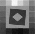
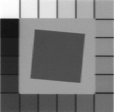
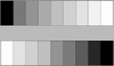

")

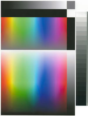
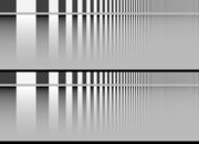
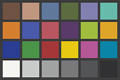
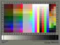
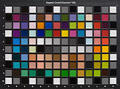
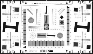
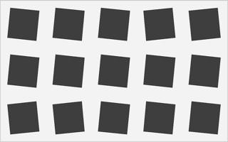
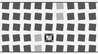
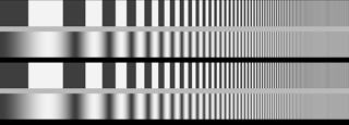
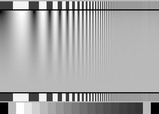

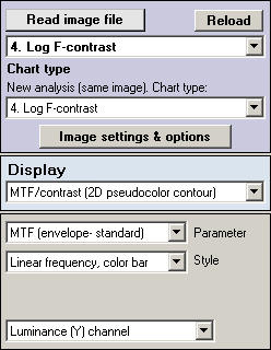

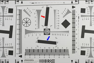


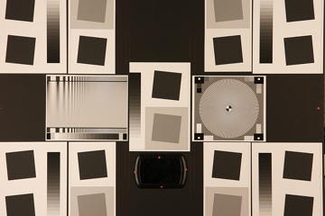
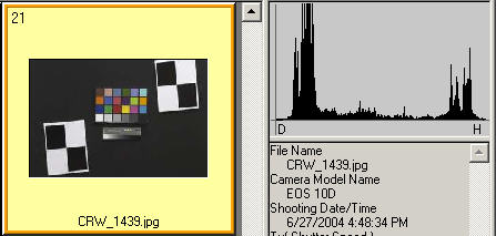
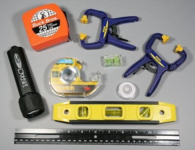
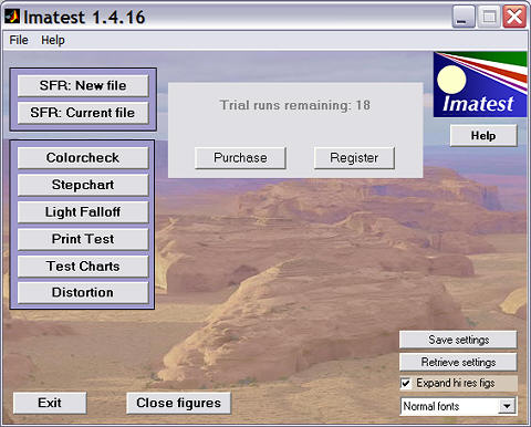
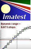

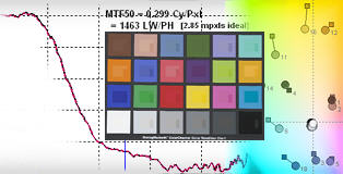
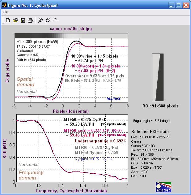

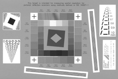
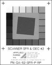
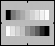
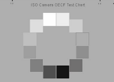
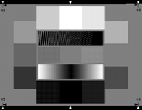
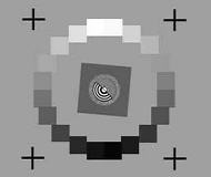
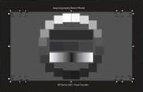
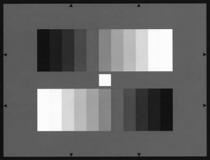
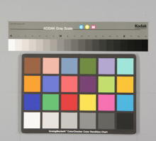
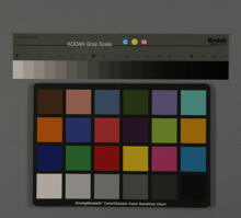

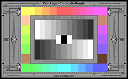
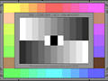
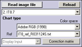
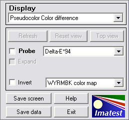
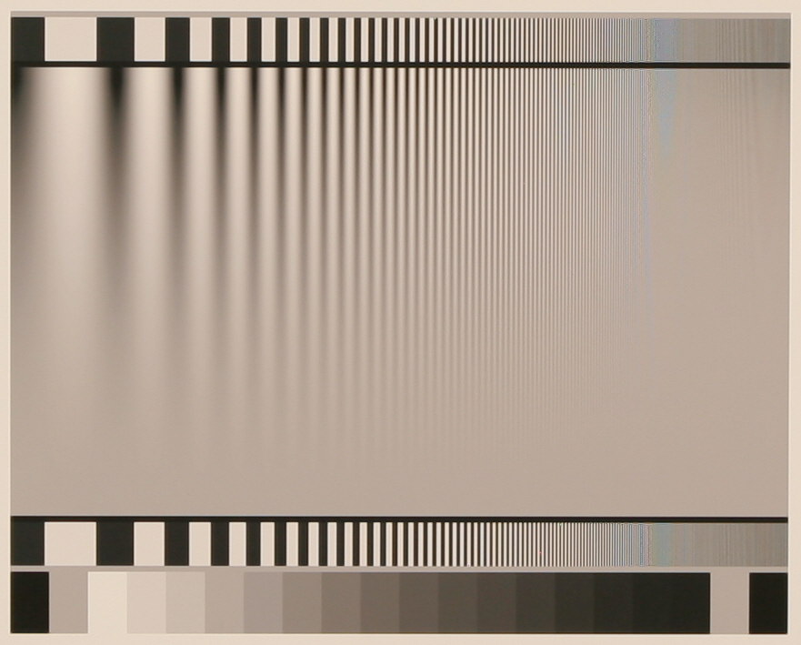
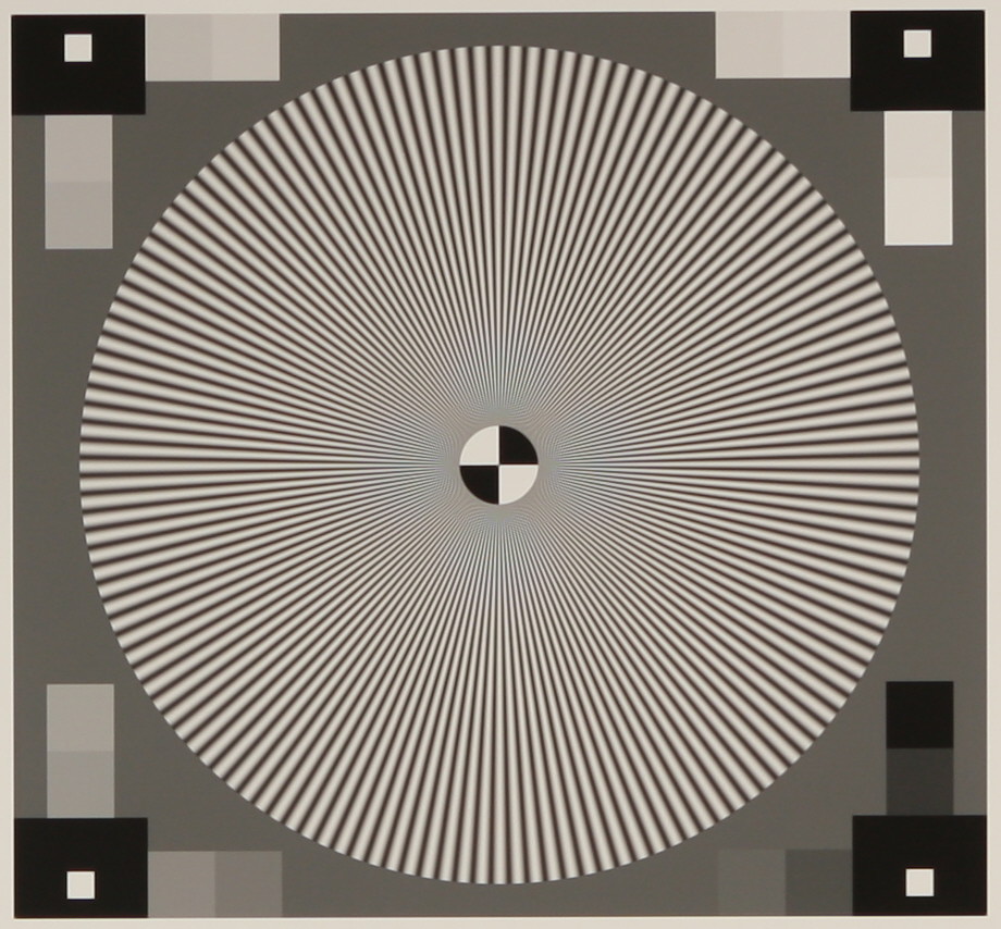
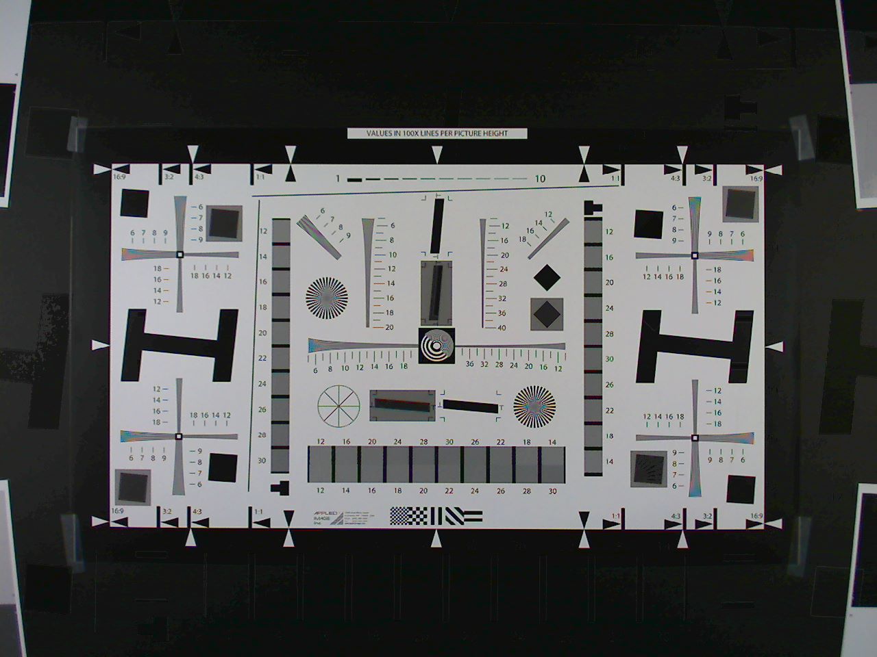
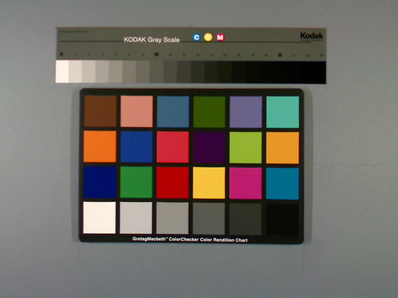
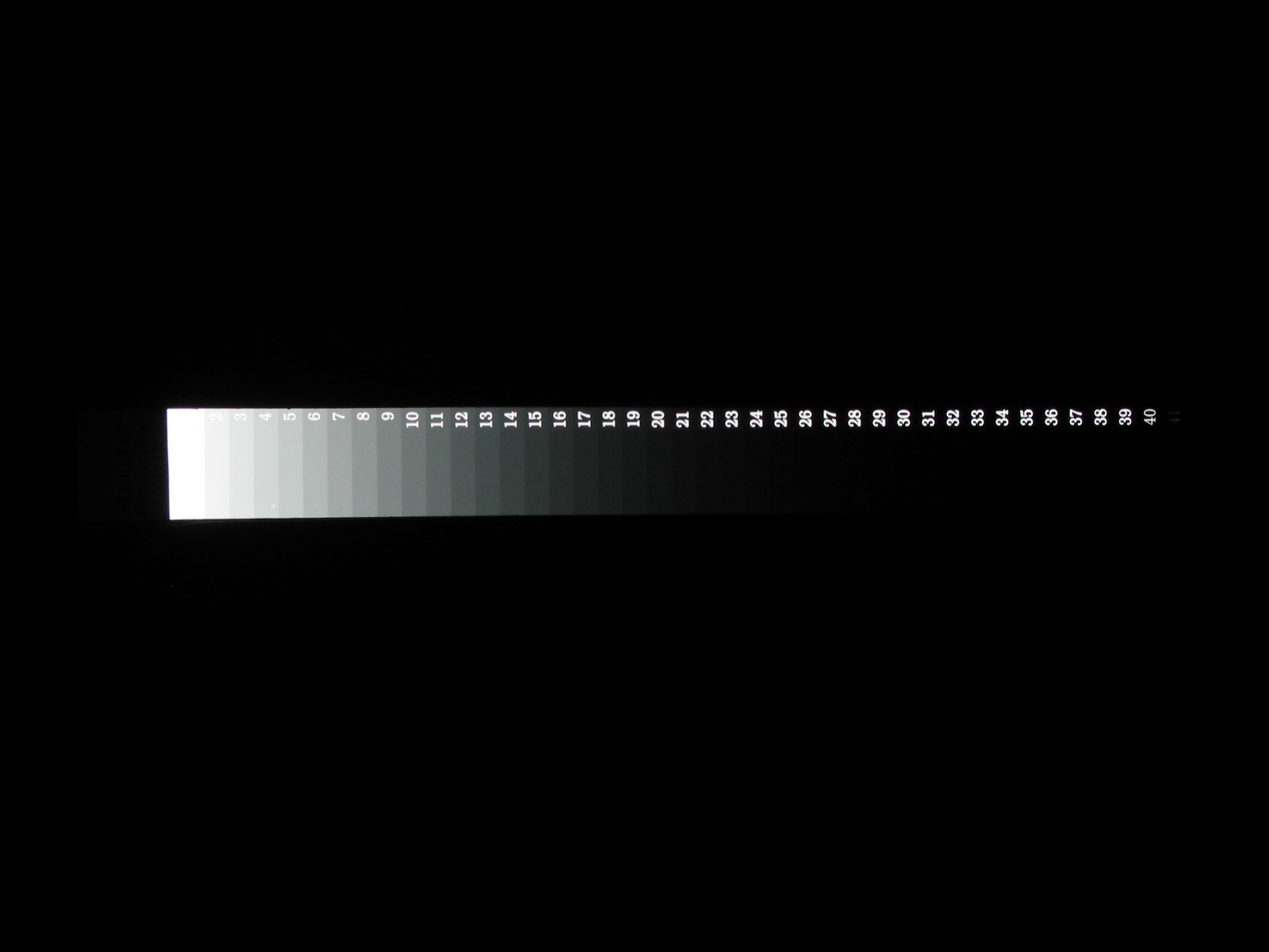
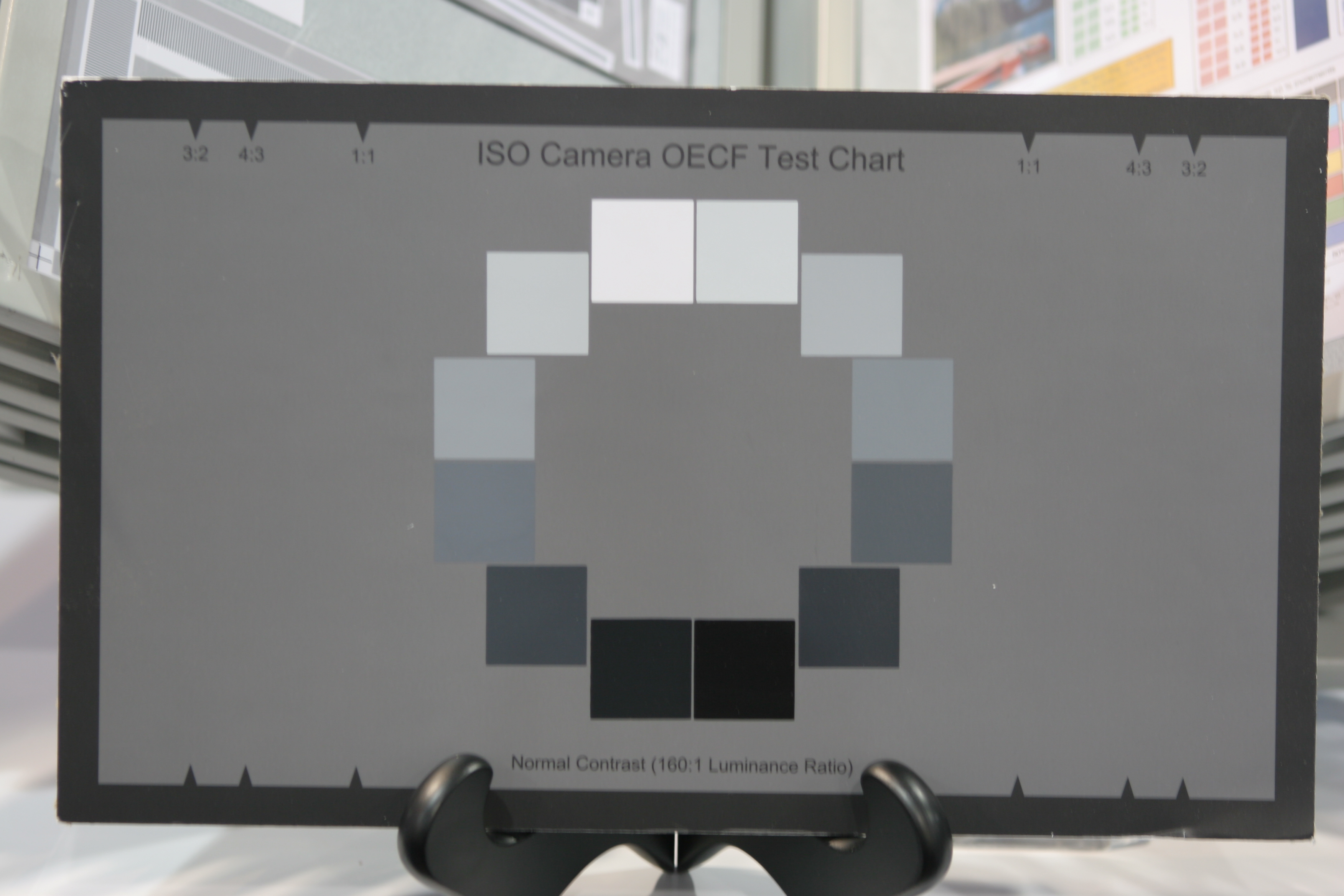
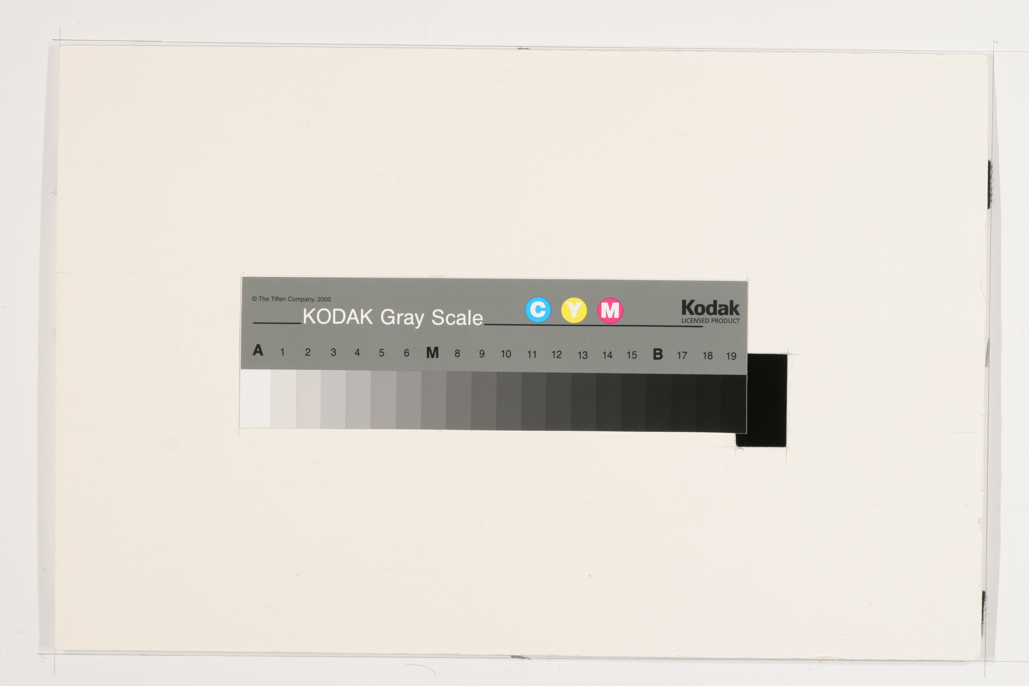
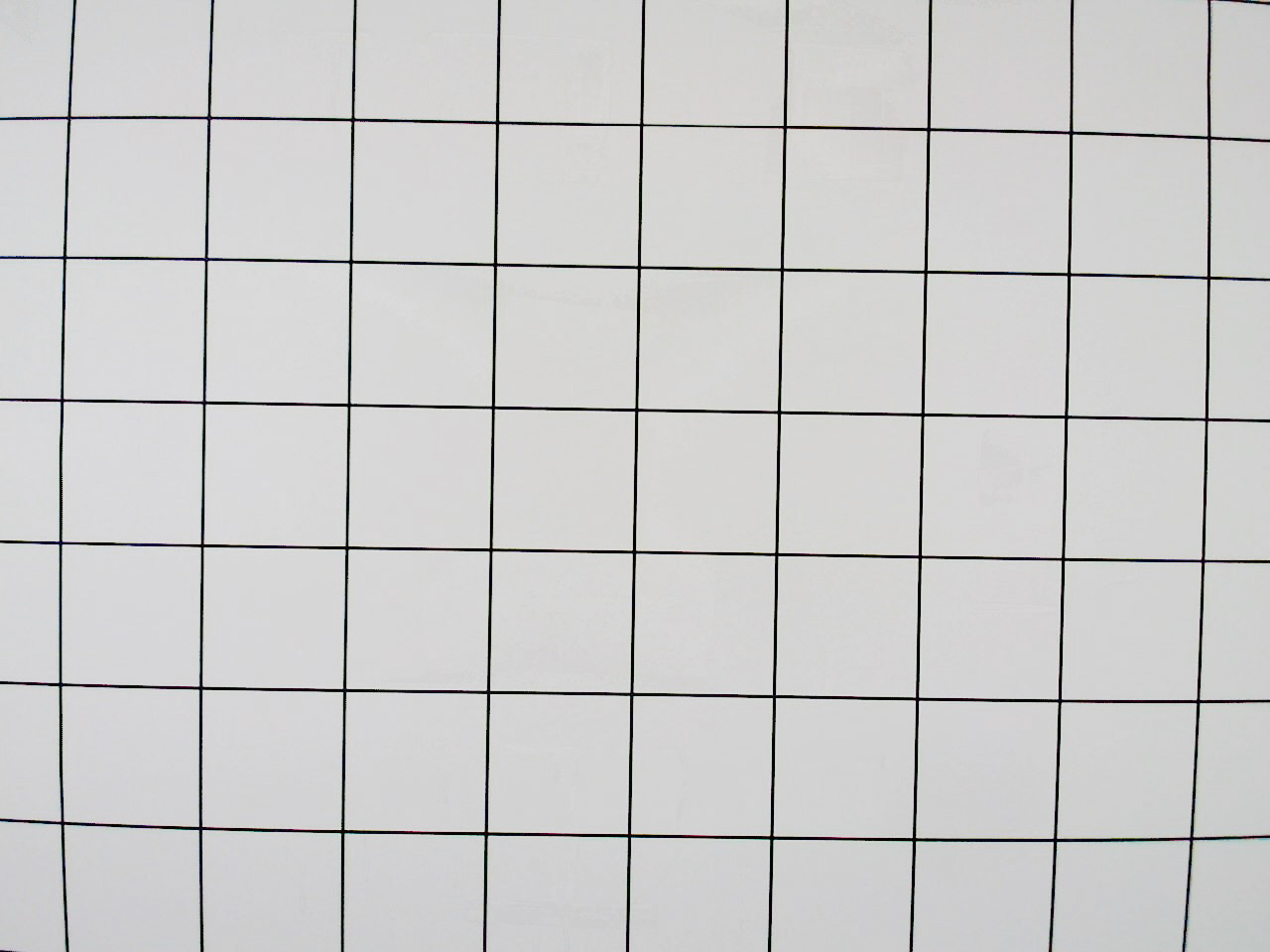
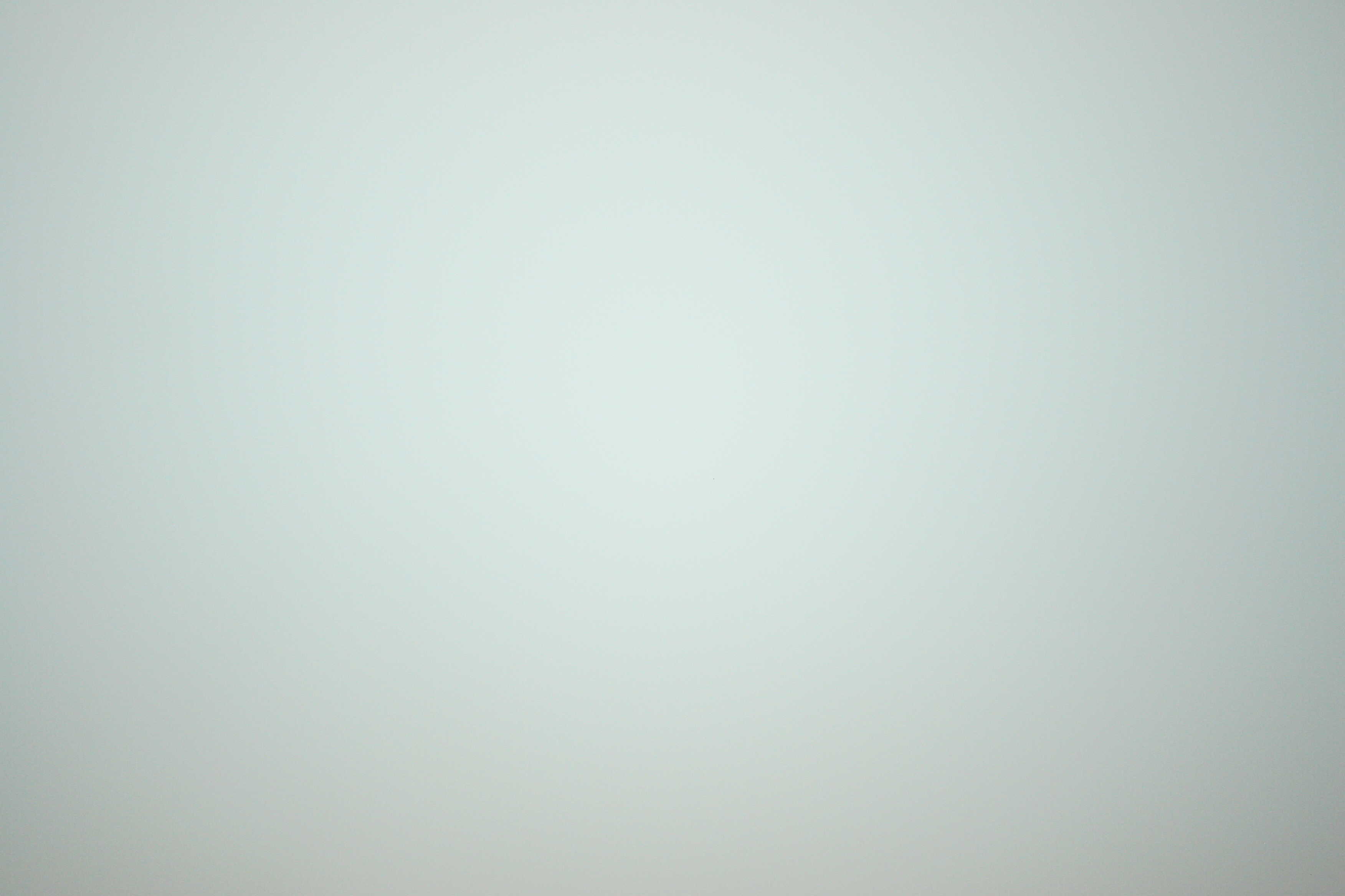
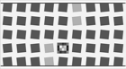
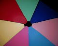
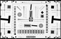
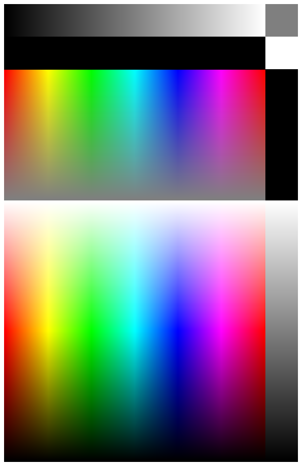
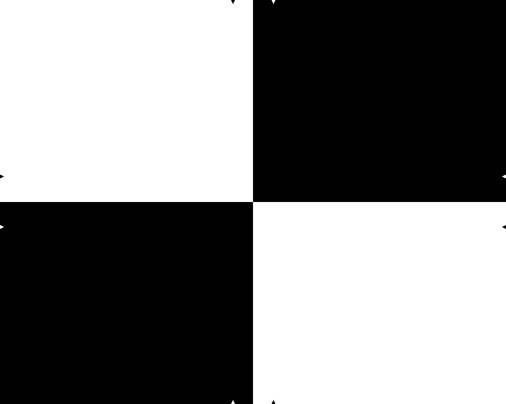
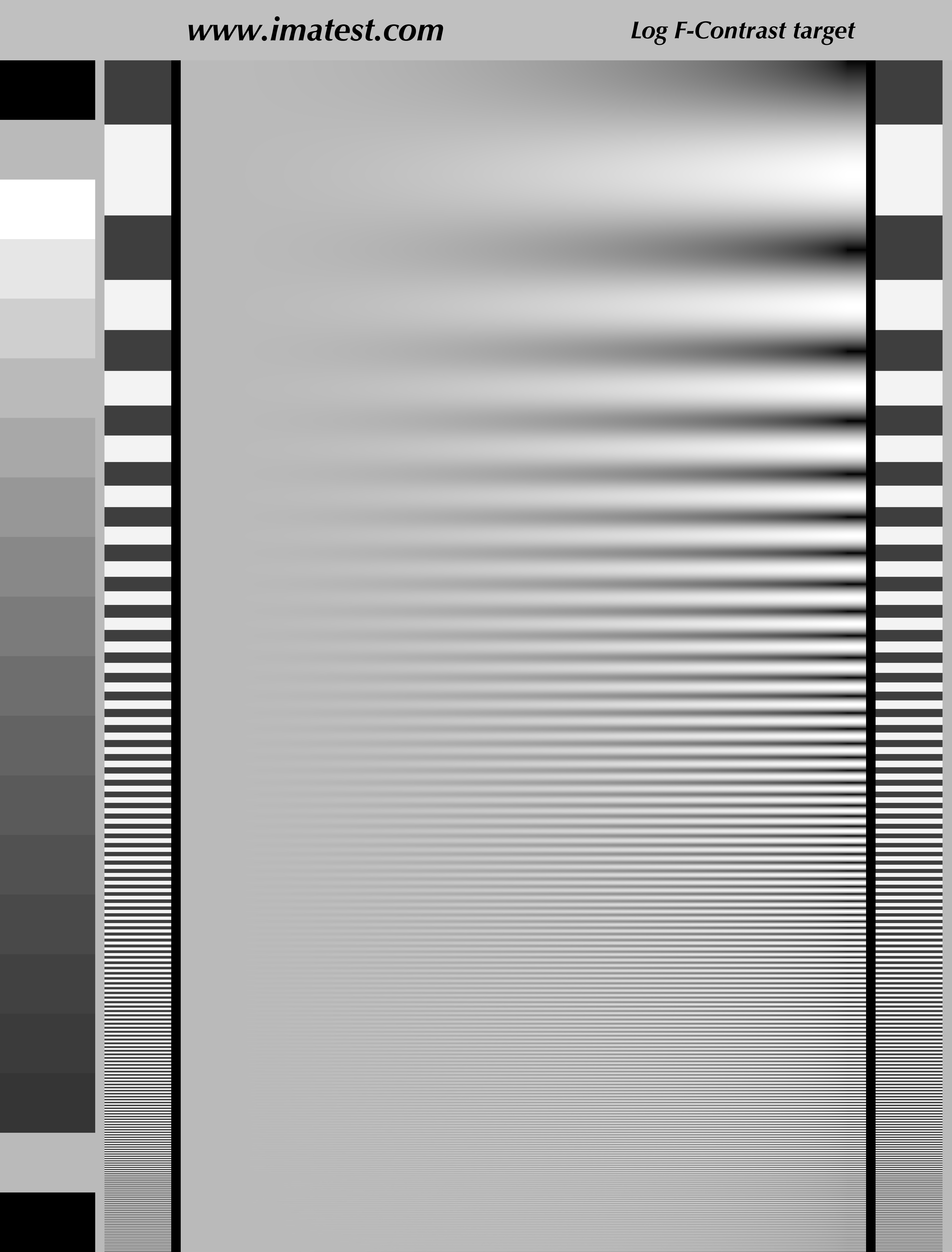