Measure visible sensor defects
The Human Visual System – Algorithm – Instructions – Settings window –
Filtering and threshold – Display options – Defective pixels – Tuning – Results
Flatfield Blemish Detect detects visible sensor defects (typically blurred (dark) spots caused by dust in front of the image sensor, but light blemishes can also be detected). To ensure that only visible blemishes are flagged— and blemishes below the threshold of visibility are not— the image is filtered by a response function derived from the Human Visual System (HVS). Filter settings are adjustable for a wide range of applications and viewing conditions. The IT version of Flatfield, which can be incorporated into automated testing systems, can significantly improve sensor yields by simultaneously minimizing false negatives and false positives.
| Read the instructions carefully! Getting the most out of Flatfield Blemish Detect requires careful tuning, which requires background knowledge. |
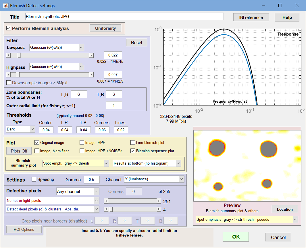
| Imatest 5.1: You can specify a circular radial limit for fisheye lenses. Imatest 3.10: Images larger than 5 megapixels can be downsampled for improved speed and reduced memory usage. |
Flatfield Blemish Detect is part of the Flatfield analysis focused on defects or blemishes, i.e., localized density variations. Settings, which are saved in imatest-v2.ini or in named ini files for Imatest IT, are described in Flatfield ini file reference.
The Human Visual System
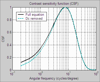
| The human eye’s Contrast Sensitivity Function (CSF), shown on the right, is a measure of the eye’s MTF response. It is limited by the eye’s optical system and cone density at high spatial (or angular) frequencies and by signal processing in the retina (neuronal interactions; lateral inhibition) at low frequencies. Various studies place the peak response at bright light levels between 4 and 8 cycles per degree.The CSF formula, which has the form k1f exp(-k2f ), is described in the page on Subjective Quality factor (SQF).
The human eye is sensitive to relative luminance differences. That’s why we think of exposure in terms of zones or f-stops, where changing exposure by one f-stop or zone means halving or doubling the light. The smallest luminance difference the eye can distinguish in bright light (ΔL) is expressed by the Weber-Fechner law, ΔL/L = 0.01 (G. Wyszecki & W. S. Stiles, “Color Science,” Wiley, 1982, pp. 567-570). This is a relative difference of 1%. The thresholds, described below, are loosely related to this number (though they’re typically considerably larger in practice— 0.03 or larger— because of the bandpass filtering). |
|
|
The coincidence In order to get good blemish readings you must
This filtering bears a curious resemblance to the contrast sensitivity function (though for practical reasons it’s not an exact replica). |
Algorithm
- The image is linearized using the equation, V = Pixel level(1/gamma), where gamma is the approximate exponent used to encode the image. Gamma is around 0.5 for standard color spaces (sRGB, Adobe RGB) and 1.0 for raw images.
- The linearized image is filtered with a bandpass filter whose frequency cutoffs (set in the input dialog box) are derived from, but not identical, to the human visual system’s Contrast Sensitivity Function. The actual bandpass must be wider to account for noise, light falloff, and a range of viewing conditions. These factors are discussed in detail below.
- The filtered image has a mean value of 0 because the highpass portion of filter removes the dc component (spatial frequency = 0).
- The filtered image is normalized (divided) by the mean of the linearized (unfiltered) image. This scales it so units are the same as ΔL/L in the Weber-Fechner law described above, i.e., a value of -0.01 means that a pixel is darker than its average surroundings by 0.01 (1%). This signal is called the “blemish-filtered” signal.
- A pixel error is detected if a blemish-filtered value is lower than minus the threshold. Example: a value lower than -0.03 for a threshold of 0.03. The number and size of contiguous (connected) errors is also calculated.
- The mean of the vertical lines is calculated by averaging columns of blemish-filtered pixels, scanned horizontally, excluding 5% of the total height at the top and bottom of the image. The mean of the horizontal lines is calculated by averaging rows of blemish-filtered pixels, scanned vertically, excluding 5% at the left and right. These lines can be displayed in the Line blemish plot. An error is detected if the absolute value of either mean is greater than the line threshold.
|
Lowpass and Highpass filtering (familiar if you have a background in Electrical Engineering)
Filters are characterized by bandwidth (typically the frequency where the ratio of output to input power (the transfer function) falls to 0.5, and by the rate of rolloff, which is more rapid for the gaussian filters than for exponential filters (selectable in the input dialog box). The word “bandwidth”, which has become widely used in English slang, has its origins in Electrical Engineering. If the original (unfiltered) image contains a tiny speck (perhaps a dead or hot pixel), a lowpass filter will broaden it and reduce its amplitude. For the human eye, the speck will be visible if its amplitude is large enough— if ΔL/L is greater than a threshold, which must be at least 0.01, as described above, for large objects with well-defined boundaries. The threshold for small objects is typically higher. |
Instructions
To prepare an image for Flatfield Blemish Detect,
- Set your camera or lens to manual focus, if available.
- Wide angle lenses, which usually have significant vignetting, are not recommended for measuring sensor defects.
- The aperture (f-stop) setting affects the results because many blemishes are caused by dust on the surface of the imaging chip, separated from the sensor by the Bayer, anti-aliasing, and infrared (IR) filters (up to 1mm). This separation blurs the dust speck. The blur radius increases as the aperture increases (as the f-number decreases). For small dust spots, the blemish amplitude decreases as the aperture increases, i.e., intensity is inversely proportional to radius.
-
Screen Pattern module for
Blemish Detect and Uniformity.Photograph an evenly illuminated uniform subject.
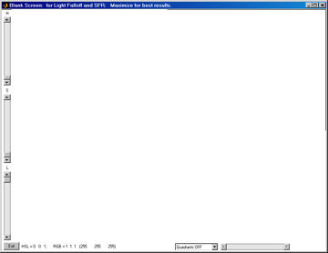
- One of the simplest ways to obtain a uniform subject is to photograph your computer monitor at a distance of 1-3 inches (2-8 cm) using the Imatest Screen Patterns module, shown on the right. Click on on the right of the Imatestmain window, then maximize the screen. You can adjust the Hue, Saturation, and Lightness (H, S, and L, which default to 0,0,1) if required.
This method works best with flat screen LCDs with wide viewing angles (not so well with laptops,which are strongly viewing angle-dependent or CRTs, due to raster scan).
- We recommend using opal diffusing glass mounted close to the lens. Opal glass is available from Edmund Optics. If a diffuser is used, a light box (fluorescent with high frequency ballast or LED) may be substituted for the monitor. (Light boxes are typically brighter but less uniform.)
- (We prefer other approaches, but this sometimes works.) Photograph an evenly-lit smooth matte sheet (white or gray). Be careful not to shade it. Outdoors illumination (shade) sometimes provides very even illumination. Getting uniform illumination can be a challenge with wide-angle lenses; it’s almost impossible to avoid shading part of the card. Opal diffusing glass is strongly recommended.
- The subject does not need to be in focus (you don’t even need a lens to measure sensor uniformity); the goal is to measure sensor uniformity, not features of the subject. For typical measurements, set exposure compensation to overexpose by about one f-stop. (You may, however, use any exposure you choose.)
- Save the image as a RAW file or maximum quality JPEG.
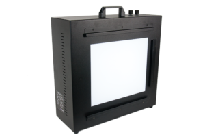 To obtain even illumination We recommend the Imatest LED Lightbox which produces uniform light with excellent spectra characteristics that can be adjusted over a wide range of brightness for illuminating transparency test charts. It can be used with Imatest Dynamic Range and other transmissive test charts. The most even illumination can be obtained with an integrating sphere from a supplier such as Gamma Scientific or Colorspace). Integrating spheres are more expensive than LED lightboxes. |
To Run Flatfield Blemish Detect
Running Flatfield Analysis from the Main Window:
- Select your Image, then click Next to Select Analysis options.
- In Analysis Options screen – open the “Uniformity” Category, and select Flat Field.
- There is a radio button at the bottom of the analysis card that allows you to select the Interactive (or Automatic) mode. Select the desired mode.
- Click Analyze – the ROI option screen will appear, (choose the desired ROI and click yes), then the Flatfield Interactive results screen will be displayed.
- There are buttons on the bottom of the page to change Settings for Uniformity and Blemish. (The settings are described in detail below. )
- In order to run Blemish analysis, be sure the Perform Blemish Analysis checkbox is selected on the Flatfield Uniformity Settings screen.
- Blemish-specific settings can be set by clicking on the Blemish button to access the Blemish Detect Settings screen.
- Use the dropdown menu on bottom left of the results screen, to choose a different output display.
- Results can be saved using the Save screen or Save Data buttons. When done, click Exit to return to Main Window.
Running Flatfield Analysis from the Classic UI:
- Start Imatest, and choose Classic UI from the Main Menu. When the Classic interface appears, click on .
- A dialog box will open and that prompt you to select input image file(s). Choose the file name, and click on the Open button.
More about Files: very large files (height x width x colors over 40 MB) may cause memory overflow problems. Files over 40 or 80 MB can be automatically reduced 1/2x linearly (using 1/4 the memory). Click Settings, Options I (in the Imatest main window) and make the appropriate setting in LARGE FILES (Uniformity, Blemish, Distortion).
|
Three cropping (ROI selection) options are available by clicking in the Imatest main window (or the Blemish Detect input dialog window). These include
| Don’t ask to crop. (Use Crop … borders settings in LF input dialog box.) |
| Select crop by dragging cursor. Ask to repeat crop for same sized image. |
| Select crop by dragging cursor. Do not ask to repeat crop. |
The second option (Select crop by dragging cursor. Ask to repeat crop for same sized image), which is similar to the ROI selection in SFR, is typically preferred.
Settings window
The Settings window opens after the image file has been selected (unless Express run is checked).
Be sure that the Perform Blemish Analysis checkbox is selected.
Settings window: used to adjust filter and threshold settings with help from the Preview
(Spot emphasis shown). We recommend experimenting with
different filter, threshold, and preview settings.
- Title Defaults to the file name. You can change it if you wish.
- Perform Blemish analysis (normally checked) When unchecked, Blemish analysis is turned off and Response and Blemish summary previews are not displayed. Uniformity analysis can still be performed. This can speed up runs considerably when blemish analysis (which uses a computationally-intensive 2D Fourier transform) is not required.
- button opens the Flatfield Uniformity Settings window. All Uniformity results can be calculated, except for histograms and fine noise detail, neither of which product numerical results that can be used in Imatest IT.
Filtering and threshold
The blue region to the left of the filter response plot contains the blemish filter and detection settings.
- Lowpass The high frequency rolloff of the filter (so named because it “passes” low frequencies). The dropdown menu specifies the equation of the rolloff: either an exponential (exp(-kf )) or a Gaussian (exp(-(kf )2)) rolloff. The exponential rolls off more slowly— is less aggressive in removing high frequencies— but resembles the human eye’s rolloff. The slider specifies the approximate cutoff frequency. The effects of the lowpass filter are visible in the high spatial frequency region on the right of the response plot and in the Preview window. Too high a frequency makes the results excessively sensitive to noise; too low a frequency can cause small (but visible) defects to be missed.
-
Highpass The low frequency rolloff of the filter. The dropdown menu specifies the equation of the rolloff: either an exponential (exp(-kf )) or a gaussian (exp(-(kf )2)) rolloff. The slider specifies the approximate cutoff frequency. The effects of the lowpass filter are visible in the low spatial frequency region on the left of the response plot and in the Preview window. Too low a frequency makes the results excessively sensitively to uneven illumination (light falloff, vignetting, etc.); too high a frequency makes can cause large (but visible) defects to be missed.
Downsampling greatly improves speed and reduces memory in blemish calculations, which use a memory-intensive 2-dimensional Fourier transform. It can be particularly valuable in manufacturing environments (with Imatest IT) that may have limited resources.
The filter response plot, to the right of the Lowpass/Highpass Filter area, shows the filter response curves. The blue (lower) curve is the combined LPF and HPF response. The black (upper) curve is the combined response normalized to a maximum value of 1.0; this is the curve used for the actual filter calculations.
-
Zone boundaries
(red lines)Zone boundaries: % of total W or H Because regions near the edges of the image may be less visually critical or may have edge-related irregularities, Blemish allows you to divide the image into nine areas for analysis, defined by pairs of vertical and horizontal dividing lines. The values entered are for locations of the vertical lines (defining left and right regions) and horizontal lines (defining top and bottom regions), expressed in percentages of total Width and Height. The illustration on the right shows both boundaries (red lines) = 6%. Blemish thresholds can be set separately for the regions.
- Thresholds can be set separately for each of the four zone groups and for lines: Center, (Left, Right), (Top, Bottom), Corners, and Lines.
- Type is the blemish type. Can be Dark (the default), Light, or Both (Dark and Light).
- Value is the absolute value of the threshold. A blemish is detected when the blemish-filtered signal level is below –threshold. (At the present time only darkened regions are considered to be blemishes.) Recall that the blemish-filtered signal has a mean of zero (due to highpass filtering, which removes DC) and has been normalized to the mean signal level (before filtering), so the threshold corresponds to ΔL/L in the Weber-Fechner law. For practical reasons (sensor noise, viewing conditions), thresholds are generally larger than 0.01. Default values are 0.02 for the center region, 0.03 for top, bottom, left, and right, 0.04 for the corners, and 0.01 for lines. Higher values are often better.
| Learn more about tuning, especially setting the Highpass and Lowpass filters, in the Tuning section, below. |
Plot (Display) options
The Preview image in the lower-right gives a 280×200 pixel preview of the filtered image. It is updated whenever filter settings are changed, making it useful for tuning. Preview displays (examples shown below) include
| Original image |
| Original image for reference. Not affected by settings. | |
| Image with blemish filter | Filtered image. Shows the effects of the filters on blemishes. Since only a small (280×200) segment of the original image is shown, does not show the suppression of long-range variation from the highpass filtering. |
| Linear pseudocolor |
The blemish-filtered image is displayed linearly in pseudocolor. |
| Spot emphasis pseudocolor |
The blemish-filtered image in pseudocolor with spot emphasis: shows deviation from the local average. Values above 1 (the local mean after filtering) are white. Values below 0.9 (0.1 below the local mean) are black. |
| Spots < center threshold pseudocolor |
The blemish-filtered image in pseudocolor showing only regions below (–) the threshold. Higher values are white. Values below -0.1 are black. |
| Linear, gray < ctr threshold pseudocolor | Similar to Linear pseudocolor (above), except that detected blemishes (levels less than (-) the center threshold) are shown in gray. |
| Spot emphasis, gray < ctr thresh pseudocolor | Similar to Spot emphasis pseudocolor (above), except that detected blemishes (levels less than (-) the center threshold) are shown in gray. |
When the Preview setting is the same as the Blemish summary plot setting, both settings have pale yellow backgrounds. Otherwise the Blemish summary plot background is pale pink (indicating that what you see won’t be what you get).
The Preview image location can be changed by pressing , and dragging the 280×200 pixel crop with the mouse. The final crop is shown in red. It should include blemishes of interest (above or below the threshold).
We strongly encourage all users to experiment with different settings—
low and high pass filter cutoffs and responses as well as preview options.
 |
 |
 |
 |
 |
The Plot region (middle-left) specifies which figures to plot. The figures are described in Detail in the Results section, below.
- Four image plots selected by checkboxes on the left display the image with different signal processing applied (Original image (none), Blem filter (LPF+HPF), HPF, HPF >Noise> (noise boosted 10X)) are illustrated below. Since the latter three images don’t contain final results, they are mostly of interest for diagnostics and finding settings.
- Line blemish plot plots the amplitude of horizontal and vertical lines in the image. Lines tend to be more visible than spots, hence they have their own threshold (default value = 0.01).
- Blemish count plot shows the sizes of contiguous (connected) blemishes. Rarely needed because the 2D blemish (summary) plot shows the blemishes and blemish statistics if Add results at bottom (no histogram) is selected.
- Blemish summary plot (pseudocolor) contains two dropdown menus (not checkboxes) just below the checkboxes listed above). This plot contains the key results from Blemish Detect, plotted in pseudocolor. Many options can be selected.
Left dropdown menu You can see what these do using the Preview window. The background is shown in pale yellow when the setting is the same as the Preview window.
Off Omit this plot. Linear Spot emphasis Blemish-filtered results greater than 1.0 are displayed as pure white. This makes it easy to locate blemishes, which can get lost in the linear display. Spots > threshold Only blemishes outside the thresholds are displayed. This provides the clearest blemish display. Linear, gray < threshold Similar to Linear (above), but blemishes (level < (-) threshold) are shown in gray. Spot emph., gray < threshold Similar to Spot emphasis, but blemishes (level < (-) threshold) are shown in gray.
Right dropdown menuNo added results The image fills the plot. Add results at bottom (no histogram) Recommended The filter response, pixel statistics, and connected blemish statistics (sorted by size) are displayed below the image. Scrollable tables are used for the statistics. Add results at bottom with histogram (slow) The filter response, pixel statistics, and a histogram of the levels are displayed below the image. The standard deviation of the image level is also displayed. NOT recommended because calculating the histogram and σ is slow.
The Settings region lets you enter settings that affect the results.
- Speedup When unchecked, some Light Falloff information (levels at sides and corners) is calculated and saved. Makes relatively little difference for run times. Leave it on if you need basic light falloff statistics in the output files.
- Gamma (Settings area). The default value of gamma, 0.5, is typical for digital cameras. Gamma is used to linearize the image. It can be measured by Stepchart using any one of several widely-available step charts. (Reflection charts are easiest to use but transmission charts can also be used to measure dynamic range.)
- Channel Selects Red, Blue, Green, or Y (luminance) channel
- Corner and side regions (default 32x32 pixels) allows you to select the areas at the corners and sides of the images to be analyzed. These affect the edge and corner level calculations, which are saved in CSV and XML output when Speedup is unchecked. Choices include 10x10 pixels, 32x32 pixels, 1% (min. 10x10), 2% (min. 10x10), 5%, and 10%. This may be removed when Blemish functionality is added to Light Falloff.
Defective pixels
| Defective (Hot and dead) pixels By checking the appropriate boxes (shown on the right) you can display hot or light pixels (red x) and/or dead or dark pixels (blue o or •). Absolute pixel threshold or Relative % threshold can be selected. Cluster detection can be included if required. |
|

- Channel Selects the channel(s) to be used for defective pixel detection. Three choices:
| Any channel |
A defective pixel is registered if any channel (R, G, B, or Y) is defective. (this detects the most defects.) |
| Selected channel |
A defective pixel is registered if the selected channel (R, G, B, or Y— selected just above the Defective pixel area), is defective |
| All channels | A defective pixel is registered if all channels (R, G, B, and Y) are defective. (This detects the fewest defects.) |
- Hot/Dead — Absolute/Relative — Cluster detection
| Detect hot or dead pixels (x or o): Absolute pixel threshold (Selections 2 and 4) |
Hot pixels are stuck at or near the sensor’s maximum value (255 in 8-bit files). Dead pixels are stuck at or near 0. Because signal processing— especially JPEG compression— often causes these values to shift, you can use the sliders to set the detection threshold between 6-255 for hot pixels and 0-249 pixels for dead pixels. (The extreme values are for measurements made on white or black fields.) Clicking on < or > at the ends of the sliders adjusts the threshold by 1. The default values are 252 and 4, respectively. |
| Detect light or dark pixels (x or o): Relative % threshold (Selections 3 and 5) |
Light pixels are more than the relative % threshold above the mean of the 8 neighbors; Dark pixels are more than the relative % threshold below the mean of the 8 neighbors. Threshold is selected by the slider to the right. |
| Cluster detection (Selections 4 and 5) |
Detect clusters of hot and/or dead pixels, where a cluster is defined as two or more adjacent defective pixels (may be absolute or relative; hot and dead are treated separately). The number of clusters and largest cluster are reported. Takes a little extra time. |
The Corners box lets you reduce sensitivity to hot and dead pixels by a factor of 2 in an nxn region set in the box.
JPEG files should be saved at the highest quality level for this feature to work well; isolated hot and dead pixels tend to be smudged at lower quality levels. Details of hot and dead pixels are presented below. You can choose whether to count a pixel as hot or dead (light or dark) if the criteria are met by any color channel (the default), all channels, or the selected channel. Details are described in Uniformity: Imatest Master.
- Crop pixels near borders (L, R, T, B) (This feature is normally disabled.) Enabled only if Don’t ask to crop. (Use Crop … borders settings in LF input dialog box.) is selected in the . If checked, the image is cropped by the number of pixels indicated near the left, right, top, and bottom borders.
Two methods of region selection
The region to be analyzed (ROI) is normally set in the coarse and fine region adjust windows, where the ROI is defined relative to the upper-left corner, not to each of the edges. So if you want a constant margin for several images (for example, you want the ROI boundaries to be 4 pixels from the borders), ROI must be set individually for each image size.
Blemish Detect offers an alternative method of specifying the ROI relative to the image boundaries: crop_borders, which is set with Crop pixels near borders near the bottom of the Blemish (or Uniformity) window when (Use Crop … borders settings in LF input dialog box.) is selected in and the Crop pixels… box is checked. Otherwise, crop_borders is ignored and the standard ROI selection is used.
Tuning
It is very important to set the key parameters of Blemish Detect so detected errors correspond to visible defects— to minimize both “false positives” and “false negatives”.
The key parameters are
- Lowpass filter function and cutoff frequency. The exponential function is closest to the eye’s response, but the Gaussian should be used if a sharper cutoff is required (typically for more aggressive noise reduction while maintaining visibility of small defects) The cutoff frequency (slider position) should be tuned so small but visible spots in a test image preview (example below) have appropriate intensity relative to larger spots and fall outside the threshold if they’re intense enough to be visible.
- Highpass filter function and cutoff frequency. The more aggressive Gaussian rolloff is generally preferred to remove light falloff and edge effects, which should not be mistaken for blemishes. The cutoff frequency (slider position) should be selected so large spots are not too light. This setting involves a tradeoff.
- Threshold values, particularly for the center region, should be set after the filter settings.
Test image
(A more sophisticated approach is under development, but the image below is a good start.)
Print or display the full-sized version of the image shown below, which you can download by clicking here or on the image itself. The image should viewed under the typical conditions for the product under development as well as for the range of angular fields of view that you expect.
Use it to set the key parameters so that spots you consider to be objectionable are above the threshold and spots that are not objectionable are not. If small spots appear to be too strong in the Blemish plot (described below), decrease the lowpass filter frequency (move the slider to the left). The preview gives you a pretty good idea of what’s happening, but the final image is definitive.
Blemish Detect calibration image. Details shown below.
Click on the image to download the full-sized version (8 megapixels; 2.5MB)
Adjusting the lowpass and highpass filters
The lowpass filter settings affect the high frequency rolloff (on the right side of the frequency response plot). The highpass filter affects the low frequency rolloff (on the left side).
The baseline for the results is in the Settings window (above), where the Lowpass filter (LPF) is set to 0.022 (Gaussian) and the Highpass filter (HPF) is set to 0.007 (Gaussian), which gave excellent overall results. In the images below, one of the filter cutoff frequencies (LPF or HPF) has been changed; the other is the same as the Settings window.
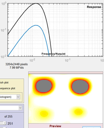 Lowpass cutoff = 0.005 (greatly reduced) |
 Lowpass cutoff = 0.222 (greatly increased) |
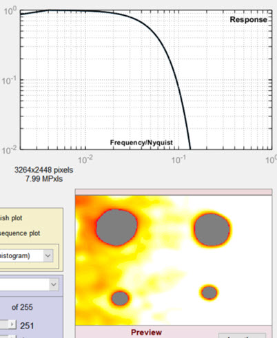 Highpass cutoff = 0.0005 (greatly reduced) |
 Overall results for Highpass cutoff = 0.0005 (greatly reduced), on left |
Results
Image figures (original and filtered)
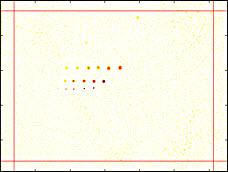
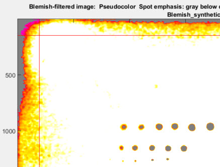
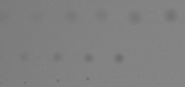
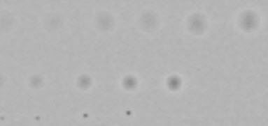
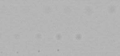
Several image figures are available. These figures are intended to facilitate the setup of filter and threshold parameters by making it convenient to compare images (original or processed) with blemish-filtered results (displayed in pseudocolor). Note that these plots are not anti-aliased, so vertical and horizontal nonuniformities (lines) may appear exaggerated in the original (unzoomed) display. To get an accurate impression, you must zoom in by clicking on an area of interest or drawing a rectangle. Double-click to zoom back out. The image illustrated below has three sequences of synthesized blemishes, differently sized, from weak to strong.
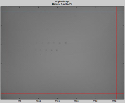
Original image (shown reduced) with synthesized blemishes
|
Original image, shown cropped with enlarged spots. When setting filter parameters (LPF and HPF cutoff frequencies as well as thresholds) this image should be observed carefully at appropriate magnification levels to verify that its appearance corresponds to the detected blemishes. |
 |
|
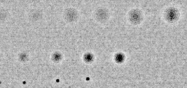
Blemish-filtered (HPF and LPF) image, cropped and enlarged This image has been filtered to remove long-range density variations (typically from vignetting) as well as noise The blemish summary plots (primary results displayed in pseudocolor), shown below, are derived directly from this image. The maximum density of spots should be closely related to the spot visibility in the unfiltered image, above. |
 |
|
Highpass-filtered image This image shows the effects of the highpass filter only. (This is an intermediate result that often won’t be needed.) |
 |
|
Highpass filtered-image with noise boosted 10X This plot maximizes the display of blemishes and noise, in distinction to the blemish-filtered plots that show blemishes, but minimize noise. Tiny defects are exaggerated. (This is an intermediate result that often won’t be needed.) |
 |
|
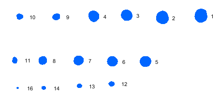
Blemish sequence plot This plot shows the blemishes and their sequence (largest to smallest). The blemish details (sizes, etc.) are in the table on the lower-right of the pseudocolor blemish blot (below). Dark blemishes are blue; light blemishes are red. |
 |
Blemish summary (pseudocolor) plot (the primary results display)
The Blemish summary (pseudocolor) plot is the primary results display— it shows blemishes clearly. Spots < (dark) threshold was selected for the plot shown below.
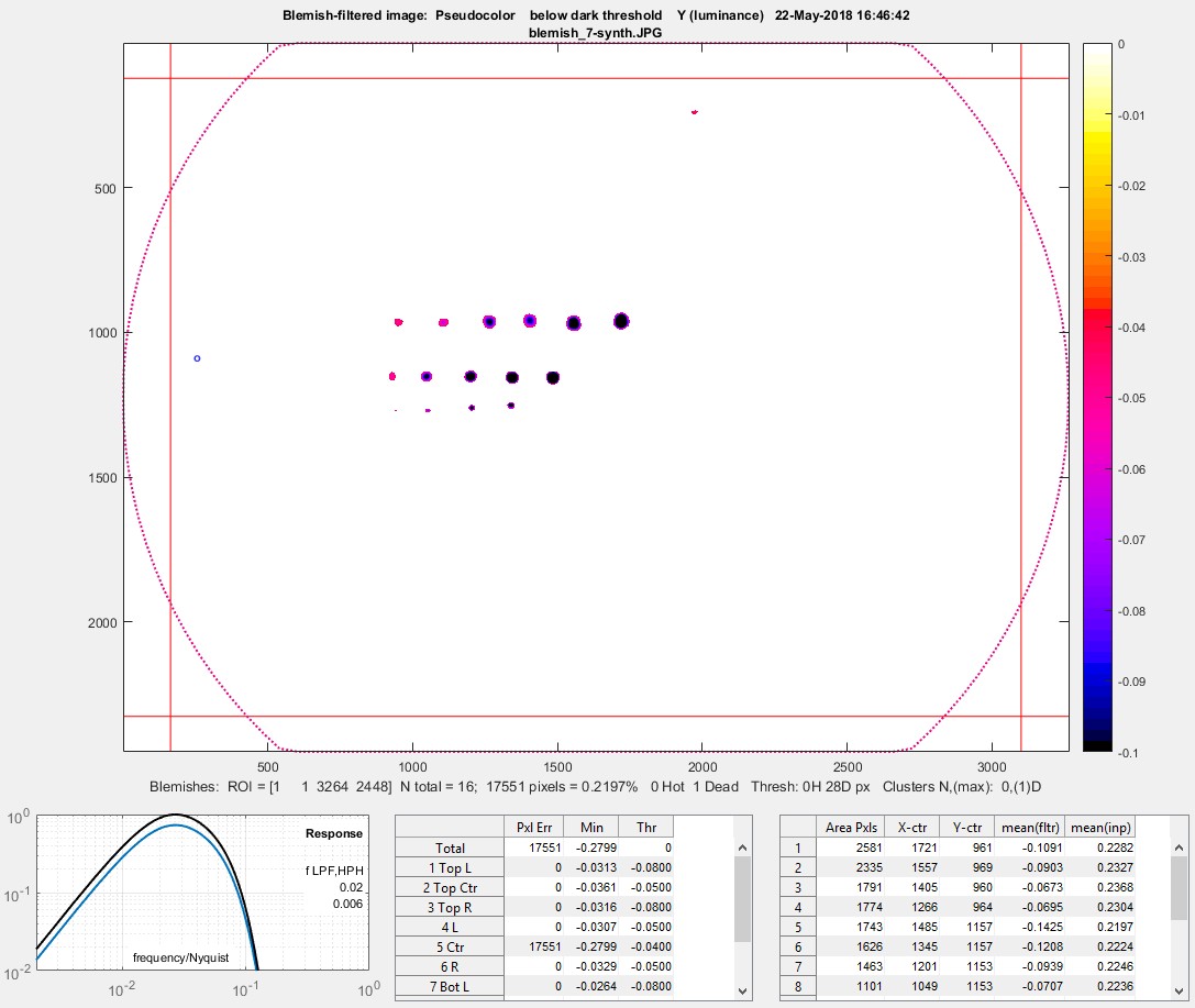
Blemish display with showing only blemishes below the threshold: the primary results of Blemish Detect.
 Enlarged blemishes (spot emphasis)
For Spots < threshold, only areas beneath the (–) blemish threshold are shown; the remainder of the image is white. Portions of this image can be enlarged, as needed.
Alternative selections include spot emphasis (shown enlarged on the right), which clamps the filtered blemish image to a maximum value of 0 and a minimum value of -0.1. This makes the (darker) blemishes much more visible than in the linear (unclamped) image below, but may not be as easy to read as the above image.
The bottom row is displayed when Add results at bottom (no histogram) is selected in the Plot area. ( Add results at bottom with histogram (slow) is not recommended because the histogram (and standard deviation) is slow to calculate and has limited value.) The filter response curve is shown on the left: the lower blue curve is the combined LPF + HPF response. The upper black curve is the response normalized for a maximum value of 1.0 (used for the calculations).
The table in the middle displays the number of errors (N Err), the minimum value (Min), and (–) the threshold level (Thr) for the image as a whole and for each of the 9 sections as well as the average vertical and horizontal lines.
The table on the right shows the area, the x, and y location (in pixels), the mean value of the blemish in the filtered image used to find the blemish (by comparing pixel levels with the threshold), and the mean value of the blemish in the linearized input image. The results are sorted by blemish size: largest first.
 Linear blemish display (enlarged blemishes)
Line blemish plot
Lines tend to be more visually prominent that spots or blemishes of similar size. For this reason, they are detected with a different threshold (generally lower; 0.005 in the image below). The plots below are for vertical and horizontal lines in the image. The same filtering is used as for spots. This plot is for an image where significant vertical banding (lines) was visible in the 10x noise boosted plot, but the banding wasn’t visible in in the original image displayed full sized (to get around anti-aliasing problems when displayed in reduced size in Matlab figures.
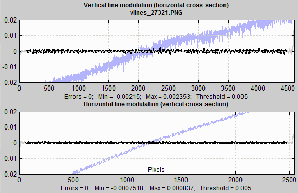
Line blemish plot
The ends of the lines, which are not included in the analysis because of end effects (in the FFT routine) are shown in light gray.
CSV and JSON output files
These output files contain additional statistics, not contained in the plots. Most have obvious meanings. For example, here is a portion of the JSON output (Light Falloff results omitted). The cool thing about JSON objects is that they can usually be parsed (decoded) by a single line of code using routines linked from the JSON page. This makes them particularly useful for post-processing (for example, determining pass/fail).
{
”blemishResults”: {
”dateRun”: “09-Jan-2012 01:24:25″,
”version”: “Imatest 3.9-Beta Master Blemish”,
”ColorChannel”: “Y (luminance)”,
”nColorChannel”: [4],
”gamma”: [0.5],
”totalImagePxls”: [7990272],
…
”freqLowpass”: [0.0175],
”freqHighpass”: [0.0055],
”filterType”: [2,2],
”thresholds”: [0.04,0.05,0.05,0.08,0.02],
”locations”: “Result,Top L,2 Top Ctr,3 Top R,4 L,5 Ctr,6 R,7 Bot L,8 Bot Ctr,9 Bot R”,
”pixelErrors”: [0,0,0,0,18760,0,0,0,0],
”minimumValue”: [-0.00705,-0.00763,-0.00765,-0.00699,-0.06241,-0.00773,-0.00684,-0.00474,-0.00726],
”maximumValue”: [0.00379,0.00422,0.00377,0.00351,0.0104,0.0052,0.00256,0.00492,0.00326],
”horizLineMin”: [-0.00173],
”horizLineMax”: [0.00116],
”N_blemish_count”: [16],
”blemishSizePxls”: [2715,2452,1905,1885,1882,1721,1551,1170,844,690,486,484,415,361,197,2],
”blemishCenter_X”: [1721.2,1557.1,1265.5,1484.8,1404.9,1344.9,1200.9,1049.1,1106.5,950.6,929.7,1340.5, …],
”blemishCenter_Y”: [961.3,969.6,964.1,1157.3,959.7,1156.7,1153,1152.6,966.6,965.5,1152,1252.7, …]
}
}
The last three data lines (“blemishSizePxls”, ff ) contain the size, x, and y-locations (in pixels) of the connected blemishes, sorted largest first.
The output formats have similar (but not identical) variable names. Contact us if you have questions, suggestions, or need additional output.
Saving results
 At the end of the run, a dialog box for saving results opens. It allows you to select figures to save and choose where to save them. The default is subdirectory Results of the image file directory. You can change to another directory by unchecking the Subfolder Results… box The selections are saved between runs.Note that several Uniformity plots are available (if they were selected to plot).
You can examine the output figures before you check or uncheck the boxes. Figures, CSV, XML, and JSON results are saved in files whose names consist of a root file name with a suffix for plot type and channel (R, G, B, or Y) and extension. Example: IMG_9875_ISO1600_RGB_f-stop_ctrG.png. The root file name defaults to the image file name, but can be changed using the Results root file name box. Be sure to press enter. For batch runs, checking Close figures after save is recommended for preventing a buildup of figures (which slows down most systems). After you click on or , the Imatest main window reappears.
Figures can be saved as either PNG files (a standard losslessly-compressed image file format) or as Matlab FIG files, which can be opened by the button in the Imatest main window. Fig files can be manipulated (zoomed and rotated), but they tend to require much more storage than PNG files, and are therefore not recommended.
CSV and XML files contain EXIF data, which is image file metadata that contains important camera, lens, and exposure settings. By default, Imatest uses a small program, jhead.exe, which works only with JPEG files, to read EXIF data. To read detailed EXIF data from all image file formats, we recommend downloading, installing, and selecting Phil Harvey’s ExifTool, as described here.
Details are described in Uniformity: Imatest Master.
The region to be analyzed is normally selected by roi, which is set in the coarse and fine region adjust windows. roi contains several groups of four values, each corresponding to the nth value of image width nwid_save and height nht_save. Each group of four roi values consists of [x1 y1 x2 y2]: the Left, Top, Right, and Bottom pixels that define the Region of Interest, defined relative to the upper-left corner, not to each of the edges. So if you want a constant margin for several images (for example, you want the ROI boundaries to be 4 pixels from the borders), roi must be set individually for each image size.
Blemish Detect offers an alternative method of specifying the ROI relative to the image boundaries: crop_borders, which is set near the bottom of the Blemish (or Uniformity) window. crop_borders contains five values: 1-4 are the margins (in pixels) relative to the L R T and B boundaries. The fifth value turns crop_borders on (1) or off (0). crop_borders is enabled when blemcrop==1 and crop_borders(5)==1. If blemcrop>1 or crop_borders(5)==0, crop_borders is ignored and roi is used for the ROI.
