Measure lens vignetting and sensor nonuniformity
Flat Field measures lens vignetting (dropoff in illumination at the edges of the image) and other image nonuniformities. For example it can measure the evenness of flash illumination (using light bounced off a white wall) or the uniformity of flatbed scanners. In Imatest, Flat Field can also analyze color shading (nonuniformity), hot and dead pixels, display a pixel level histogram, a grid (sector) plot, and a detailed image of fine nonuniformities (i.e., sensor noise). These features are described in Using Flat Field, Part 2.
Flat Field Interactive is the interactive equivalent of Flatfield. Use it when you want to examine an image in detail.
Partial support for the EMVA-1288 standard (temporal noise and spatial nonuniformities) is included in Imatest 2020.2. More details.
|
News: Imatest 22.1: The Flat Field module combines functionality from the modules formerly known as Uniformity and Blemish Detect Imatest 2020.2: Nonuniformity measurements (PRNU and DSNU) based on the EMVA 1288 machine vision standard are now supported. |
 Instructions
To prepare an image for Flat Field,
- If possible, set your camera or lens to manual focus and focus it at infinity (the worst case for light falloff).
- Photograph an evenly illuminated uniform subject.
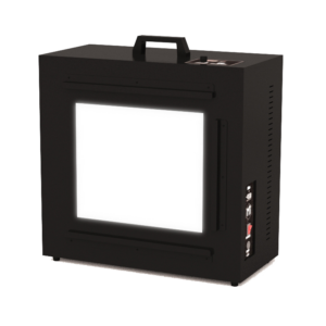
- To obtain even illumination we recommend an Imatest LED LIghtbox. There are several models. Features excellent illumination uniformity (90-95%), dimming over a range of 30 lux to 10,000 lux in standard models (with options as low as 1 lux and up to 100,000 lux), selectable color temperatures (3100K, 4100K, 5100K, 5500K, 6500K, NIR 850nm, NIR 940nm), and can be used with Imatest Dynamic Range and other transmissive charts. Imatest lightboxes are compared here.
|
The following techniques— an LCD monitor (most have flicker or have a fine structure) or a flat reflected sheet (hard to illuminate evenly) are no longer recommended. We’ve kept the instructions only for reference. 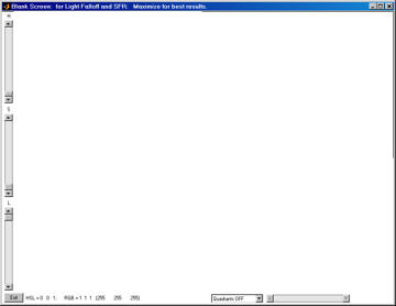 Imatest Screen Patterns display
|
- The subject does not need to be in focus (you don’t even need a lens to measure sensor uniformity); the goal is to measure lens light falloff and/or sensor uniformity, not features of the subject. For typical measurements, set exposure compensation to overexpose by about one f-stop. (You may, however, use any exposure you choose.)
- Save the image as a RAW file or maximum quality JPEG.
Running Flatfield Analysis
Running Flatfield Analysis in the New Main Window:
- Select your Image, then click Next to Select Analysis options.
- In Analysis Options screen – in Targets, open the “Uniformity/Blemish” Category, and select Flat Field.
- There is a radio button at the bottom of the analysis card that allows you to select the Interactive (or Automatic) mode. Select the desired mode.
- Click Analyze – the ROI option screen will appear, (choose the desired ROI and click yes), then the Flatfield Interactive results screen will be displayed.
- There are buttons on the bottom of the page to change Settings for Uniformity and Blemish. (The settings are described in detail below.)
- Use the dropdown menu on bottom left of the results screen, to choose a different output display.
- Results can be saved using the Save screen or Save Data buttons. When done, click Exit to return to Main Window.
Running Flatfield Analysis from the Classic UI:
- Start Imatest, choose Classic UI from the Main Menu. When the Classic interface appears, click on .
- A dialog box will open and that prompt you to select input image file(s).
More About Files:
- Very large files (height x width x colors over 40 MB) sometimes caused memory overflow problems with (older) 32-bit systems. Files over 40 or 80 MB can be automatically reduced 1/2x linearly (using 1/4 the memory). Click Settings, Options III (in the Imatest main window) and make the appropriate setting in LARGE FILES (Uniformity, Distortion). This should be unnecessary with recent versions of Imatest.
- Open the image file.
Multiple file selection Several files can be selected in Imatest Master using standard Windows techniques (shift-click or control-click). Depending on your response to the multi-image dialog box you can combine (average) several files or run them sequentially (batch mode). Combined (averaged) files are useful for measuring fixed-pattern noise (at least 8 identical images captured at low ISO speed are recommended). The combined file can be saved. Its name will be the same as the first selected file with _comb_n appended, where n is the number of files combined. Batch mode allows several files to be analyzed in sequence. There are three requirements. The files should (1) be in the same folder, (2) have the same pixel size, and (3) be framed identically. The input dialog box for the first run is the same as for standard non-batch runs. Additional runs use the same settings. Since no user input is required they can run extremely fast. Caution: Imatest can slow dramatically on most computers when more than about twenty figures are open. For this reason we recommend checking the Close figures after save checkbox, and saving the results. This allows a large number of image files to be run in batch mode without danger of bogging down the computer. Three cropping (ROI selection) options are available by clicking in the Imatest main window. These include
1. Enable “Crop pixels near borders” in Settings box. (Don’t ask to crop.) 2. Select crop (ROI) by dragging cursor. Ask to repeat crop for same sized image [default]. 3. Select crop (ROI)by dragging cursor. Do not ask to repeat crop. 4. Automatically select crop for image surrounded by a dark boundary. The second option (Select crop by dragging cursor. Ask to repeat crop for same sized image), which is similar to the ROI selection in SFR, is typically preferred

Input dialog box in Imatest Master
The settings described below are available in Imatest Studio, i.e., they appear in all Imatest versions. Additional settings are described in Using Flat Field, Part 2.
- Title Defaults to the file name. You can change it if you wish.
- Contour plots (Plot area; on by default). Often set to Display pixel and f-stop contours (two plots), but may be turned off or set to display only. Available settings are
| No contour plots |
| Display pixel and f-stop contours |
| Display pixel contours only |
| Display f-stop contours only |
- Contour plot display options Eight display options are available. 3D plots are not generally recommended because they can be slow. Normalized refers to the first (level) plot only (not to the displayed numeric results).
| Contours superposed on image (not normalized) |
| Contours superposed on image (normalized to 1) |
| Pseudocolor with colorbar (not normalized) |
| Pseudocolor with colorbar (normalized to 1) |
| 3D pseudocolor w/colorbar (not normalized) |
| 3D pseudocolor w/colorbar (normalized to 1) |
| 3D pseudocolor shaded w/colorbar (not normalized) |
| 3D pseudocolor shaded w/colorbar (normalized to 1) |
- Scaling options
| Auto or manual scaling: Set with Scaling. | Scaling set by button. |
| Scaling: 0 – 1 or 255: -4 – 0 f-stops | Fixed scaling: 0 – 1 or 255 for Luminance pixel plot; -4 – 0 f-stops for f-stop plot. |
| Scaling (min – max) | Fully automatic scaling. |
-
Manual scaling for contour plots
Contour plot scaling Scale to 1 or Scale to 255
sets the scaling for the pixel level (the first) contour plot.
- : Opens a dialog box that lets you select manual or automatic scaling for the two contour plots. Minimum and Maximum set the scale when Auto scaling is unchecked.
- Extra smoothing applies extra smoothing to the contour plots, making them less susceptible to variations from noise (and faster to plot). Strongly recommended. Uncheck this box only for compatibility with older results.
- Speedup When checked, several results (those that require significant calculation time) are not calculated (and hence not saved in the CSV output file) if the corresponding plot is not selected. This can save significant time in production environments. If you need to use Speedup, you should run Flat Field with and without Speedup checked and examine the CSV output file to see if it contains the results you require.
- Corner and side regions (default 32x32 pixels) allows you to select the areas at the corners and sides of the images to be analyzed. These affect the numeric readouts below the plots (example: Corners: worst = …). Choices include 10x10 pixels, 32x32 pixels, 1% (min. 10x10), 2% (min. 10x10), 5%, and 10%.
- Location Location of corner and side regions in units of image height (0, 1%, 2%, 5%, 10%, 15%, 20%). 0% was always implied prior to Imatest 3.8 (corner and side regions always abutted the image boundaries).
- Gamma (Settings area). The default value of gamma, 0.5, is typical for digital cameras. Gamma affects the second figure (the light falloff measured in f-stops); it has no effect on the first figure. Gamma can be measured by Stepchart using any one of several widely-available step charts. (Reflection charts are easiest to use but transmission charts can also be used to measure dynamic range.) Some issues in calculating gamma are discussed below the second figure.
- Crop pixels near borders (L, R, T, B) (Settings area). Available only if Don’t ask to crop. (Use Crop … borders settings in LF input dialog box.) is selected in the in the Imatest main window. If checked, the image is cropped by the number of pixels indicated near the left, right, top, and bottom borders.
- Crop pixels near borders (L, R, T, B) (This feature is normally disabled.) Enabled only if Don’t ask to crop. (Use Crop … borders settings in LF input dialog box.) is selected in the Options I. If checked, the image is cropped by the number of pixels indicated near the left, right, top, and bottom borders.
Two methods of region selection
The region to be analyzed (ROI) is normally set in the coarse and fine region adjust windows, where the ROI is defined relative to the upper-left corner, not to each of the edges. So if you want a constant margin for several images (for example, you want the ROI boundaries to be 4 pixels from the borders), ROI must be set individually for each image size.
Blemish Detect offers an alternative method of specifying the ROI relative to the image boundaries: crop_borders, which is set with Crop pixels near borders near the bottom of the Uniformity (or Blemish) window when (Use Crop … borders settings in LF input dialog box.) is selected in and the Crop pixels… box is checked. Otherwise, crop_borders is ignored and the standard ROI selection is used.
The following options are discussed in detail in Flat Field instructions: Imatest Master .
- Channel (Settings area) You can choose between Red, Blue, Green, and Y (luminance) channel
- Hot and dead pixels (Settings area) By checking the appropriate boxes you can display hot pixels (redx) and/or dead pixels (blue •). Hot pixels are defined in an absolute sense: stuck at or near the sensor’s maximum value (255 in 8-bit files) and dead pixels are stuck at or near 0, or in a relative sense. You can choose between hot/dead pixel detection in any channel, all channels or the selected channel.
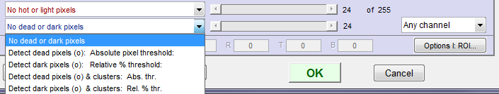 Because signal processing— especially JPEG compression— can cause these values to shift, you can use the sliders to set the detection threshold between 6-255 for hot pixels and 0-249 pixels for dead pixels. (The extreme values are for measurements made on white or black fields.) Clicking on or at the ends of the sliders adjusts the threshold by 1. The default values are 252 and 4, respectively. Settings are saved between runs. JPEG files must be saved at the highest quality level for this feature to work; isolated hot and dead pixels tend to be smudged at lower quality levels. Details are described in Flat Field part 2.
- (Plot area)
- Color shading displays color nonuniformity. Several options are available.
- Color uniformity profiles displays R, G, and B values (or ratios— several options available) along the diagonals and horizontal and vertical center lines.
- Display Histogram displays histograms of R, G, and B channels.
- Fine detail plot displays a detailed figure of noise and sensor uniformity with an option for spot detection.. The calculation can be slow and uses lots of memory. To a large extent it has been replaced by Blemish Detect. Details in Flat Field: Imatest Master.
Results
Luminance contour plot
shows normalized pixel level contours for the image file luminance channel. A maximum value of 1 corresponds to pixel level = 255 for image files with a bit depth of 8 or 65535 for a bit depth of 16. Some illumination nonuniformity is evident in the plot: the top is brighter than the bottom. The image is smoothed (lowpass filtered) before the contours are plotted. The side and corner regions are shown as red rectangles. The approximate location of the maximum luminance is indicated by a yellow O.

Luminance (relative pixel level) contour plot
The text displays the maximum unnormalized pixel level for the luminance channel, the worst and mean corner values (in unnormalized pixel levels and as a percentage of maximum), and the side values. Selected EXIF data is shown on the right. Two hot and two dead pixels (which were simulated) were detected with thresholds of 243 and 12 (pixels), respectively. The crop (Left, Right, Top, Bottom) is shown just below. Details below.
 The setting for correcting light falloff in the Picture Window Pro Light falloff transformation is also given. The PW pro Light Falloff dialog box is shown on the right. Film Size (mm) remains at 36 (the PW Pro default value: the width of a 35mm frame). Picture Window Pro is the powerful and affordable photographic image editor that I use for my own work. The Lens Focal Length is rarely the exact focal length of the lens.
Light falloff depends on the lens aperture (f-stop) as well as a number of lens design parameters. Lenses designed designed for digital cameras, where the rays emerging from the rear of the lens remain nearly normal (perpendicular) to the sensor surface, tend to have reduced light falloff. For aesthetic purposes I generally recommend undercorrecting the image, i.e., using a larger Lens Focal Length. This makes the edges somewhat darker, which is usually pleasing. Ansel Adams routinely burned (darkened) the edges of his prints. Part of the reason was that he had to compensate for light falloff from his enlarger (when he wasn’t contact printing).
“My experience indicates that practically every print requires some burning of the edges, especially prints that are to be mounted on a white card,
as the flare from the card tends to weaken visually the tonality of the adjacent areas. Edge burning must never be overdone…”
—Ansel Adams, “The Print,” p. 66. 1966 edition.
(Note: light falloff in optical enlargers would tend to lighten edges of the print— not an issue with digital prints.)
f-stop contour plot
shows image file luminance contours, measured in f-stops, normalized to a maximum value of 0. A pseudocolor display with color bar has been selected. The colors in the color bar are fixed: colors always vary from white at 0 f-stops to black at -4 f-stops and darker. For this plot to be accurate, a correct estimate of gamma (the camera’s intrinsic contrast) is required. Gamma is measured by Stepchart, using any one of several widely-available step charts, or by Colorcheck.

F-stop contour plot in pseudocolor (normalized)
Gamma can be tricky to measure for several reasons. (1) Many cameras have complex response curves, for example, “S”-curves superposed atop gamma curves. This means that gamma can vary with brightness. (2) Some cameras employ adaptive signal processing in their RAW conversion algorithms. This increases contrast (i.e., gamma) for low contrast subjects and decreases it for contrasty subjects. This improves pictorial image quality for a wide range of scenes, but makes measurements difficult, especially since Uniformity targets have the near-zero contrast.
Both contour plots are available as 3D plots (Master-only). The following 3D plot is unnormalized and shaded. 3D plots are rarely used because they are slow (but they can be pretty).

3D shaded pseudocolor F-stop contour plot (unnormalized)
The f-stop falloff in the second plot is derived from the equations,
Pixel level = k1 luminanceγ ; Luminance = k2 pixel level1/γ and
F-stop loss = log2(luminance ratio) = 3.322 log10(luminance ratio)
where luminance ratio is the ratio of the maximum luminance to the luminance in the area of interest, for example, the mean value of the corners.
Example: The first and second figures, above, are derived from the same image file. In the first figure, the mean pixel level at the corners relative to the center is 0.666/0.905 = 0.736 (73.6%). Since γ is assumed to be 0.5 (fairly typical of encoding gamma of digital cameras, the exposure at the corners relative to the center is 0.7361/γ = 0 .7362 = 0.5416. The corresponding f-stop loss = log2(0.5416) = 3.322 log10(0.5416) = -0.885 f-stops. There is a slight discrepancy with the second figure, which calculates the mean at the corners (0.894 f-stops) after taking the logarithm to convert results into f-stops.
Additional figures are illustrated in Flat Field Figure 2.
CSV and JSON output files
The .CSV output file contains additional statistics. Most have obvious meanings.
- Image pixels contains the width, height, and total size in pixels. Hot and Dead pixels show the total count and the fraction (divided to total pixels)
- The x and y coordinates of the hot and dead pixels are listed. The maximum is 100. Coordinates are in pixels from the top-left.
Contact Imatest if you need additional CSV or JSON output. The JSON output file contains results similar to the .CSV file. Its contents are also largely self-explanatory. It is stored in [root name].json.
Saving results
 At the end of the run, a dialog box for saving results appears. It allows you to select figures to save and choose where to save them. The default is subdirectory Results in the data file directory. You can change to another existing directory by unchecking the Save Results… check box. The selections are saved between runs.
You can examine the output figures before you check or uncheck the boxes. Figures, CSV, XML, and JSON results are saved in files whose names consist of a root file name with a suffix for plot type and channel (R, G, B, or Y) and extension. Example: IMG_9875_ISO1600_RGB_f-stop_ctrG.png. The root file name defaults to the image file name, but can be changed using the Results root file name box. Be sure to press enter. For batch runs, checking Close figures after save is recommended for preventing a buildup of figures (which slows down most systems). After you click on or , the Imatest main window reappears.
Figures can be saved as either PNG files (a standard losslessly-compressed image file format) or as Matlab FIG files, which can be opened by the button in the Imatest main window. Fig files can be manipulated (zoomed and rotated), but they tend to require much more storage than PNG files, and are therefore not recommended.
The CSV and XML files contain EXIF data, which is image file metadata that contains important camera, lens, and exposure settings. By default, Imatest uses a small program, jhead.exe, which works only with JPEG files, to read EXIF data. To read detailed EXIF data from all image file formats, we recommend downloading, installing, and selecting Phil Harvey’s ExifTool, as described here.
Links
Vignetting by Paul van Walree, who has excellent descriptions of several of the lens (Seidel) aberrations and other causes of optical degradation.
