Sharpness: What is it and how is it measured?
This post introduces sharpness and its measurements.
| Modulation Transfer Function |
Spatial Frequency Units |
Summary metrics |
MTF Measurement Matrix |
Slanted-edge |
|---|
Introduction | Visualizing Sharpness | Rise Distance and Frequency Domain | Modulation Transfer Function
Spatial Frequency Units | Summary metrics | MTF measurement Matrix| Slanted-Edge measurement | Edge angles
Slanted-Edge modules | Edge contrast and clipping | Slanted-Edge algorithm | Differences with ISO
Noise reduction | Related sharpness techniques | Key takeaways | Additional resources
Introduction
|
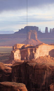
Sharpness is a key image quality factor: it determines how much detail an image can convey. The image on the right illustrates the effects of reduced sharpness (from running Image Processing with one of the Gaussian filters set to 0.7 sigma). Device or system sharpness is measured as a Spatial Frequency Response (SFR), also called Modulation Transfer Function (MTF). MTF is the contrast at a given spatial frequency (measured in cycles or line pairs per distance) relative to low frequencies. The 50% MTF frequency correlates well with perceived sharpness— much better than the old vanishing resolution measurement, which indicated where the detail wasn’t. Imatest’s primary sharpness measurement uses slanted-edge patterns analyzed by SFRplus, eSFR ISO , SFRreg, or Checkerboard which have automated region detection. SFR, can be used for manually selected SFR regions. Analysis can be performed on targets you can purchase or print with the Imatest Test Charts module. Concise instructions are found in How to test lenses with Imatest.
Several alternative patterns, which cause cameras to apply differing amounts of sharpening and noise reduction, can be used for measuring MTF. All require more real estate than the slanted-edge. They include |
|
- Log Frequency, which uses a sine pattern chart that increases in frequency logarithmically. It provides a check on the slanted-edge method. More direct but less accurate,
- Log F-Contrast, excellent for examining loss of detail due to noise reduction,
- Star Chart, a multi-directional sinusoidal pattern,
- Random/Dead Leaves, which measures texture sharpness. The Scale-invariant random pattern minimizes sharpening and maximizes noise reduction. The Dead Leaves pattern is more representative of typical images.
The perceived sharpness of a pictorial print or display is measured by Subjective Quality Factor (SQF) or Acutance, which are derived from MTF, the Contrast Sensitivity Function of the human eye, and viewing conditions.
The MTF Measurement Matrix compares the different methods.
System sharpness is affected by the lens (design and manufacturing quality, position in the image field, aperture, and (for zoom lenses) focal length), sensor (pixel count and anti-aliasing filter), and signal processing (especially sharpening and noise reduction). In the field, sharpness is affected by camera shake (a good tripod can be helpful), focus accuracy, and atmospheric disturbances (thermal effects and aerosols).
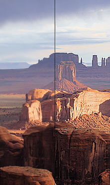
Some lost sharpness can be restored by sharpening, but sharpening has limits. It can’t restore detail where MTF or SNR (Signal-no-Noise Ratio) is very low (under about 10%). Oversharpening, illustrated on the right, above,can also degrade image quality (especially at large magnifications) by causing “halos” to appear near contrast boundaries. Images from many compact digital cameras and phones are oversharpened.
Visualizing Sharpness
Sharpness determines the amount of detail an imaging system can reproduce. It is defined by the boundaries between zones of different tones or colors.

Figure 1. Bar pattern: Original (upper half of figure) with lens degradation (lower half of figure)
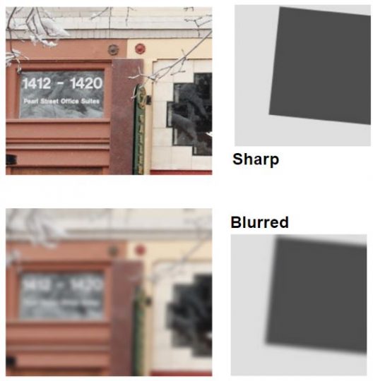
Figure 2. Sharpness example on image edges from MTF Curves and Image Appearance
In Figure 1, sharpness is illustrated with a bar pattern of increasing spatial frequency. The top portion of the figure is sharp and its boundaries are crisp; the lower portion is blurred and illustrates how the bar pattern is degraded after passing through a simulated lens.
Note: All lenses blur images to some degree.
Sharpness is most visible on features like image edges (Figure 2) and can be measured by the edge (step) response.
Several methods are used for measuring sharpness that include the 10-90% rise distance technique, modulation transfer function (MTF), special and frequency domains, and slanted-edge algorithm.
Rise Distance and Frequency Domain
Image sharpness can be measured by the “rise distance” of an edge within the image.
With this technique, sharpness can be determined by the distance of a pixel level between 10% to 90% of its final value (also called 10-90% rise distance; see Figure 3).
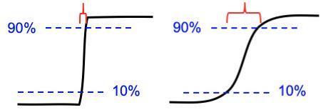
Figure 3. Illustration of the 10-90% rise distance on blurry and sharp edges
Rise distance is not widely used because there is no convenient way of calculating the rise distance of an imaging system from the rise distances of its individual components (i.e., lens, digital sensor, and software sharpening).
To overcome this issue, measurements are made in the frequency domain where frequency is measured in cycles or line pairs per distance (millimeters, inches, pixels, image height, or sometimes angle [degrees or milliradians]).
In the frequency domain, a complex signal (audio or image) can be created by combining signals consisting of pure tones (sine waves), which are characterized by a period or frequency (Figure 4). The response of a complete system is the product of the responses of each component.
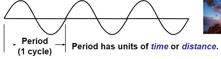
Figure 4. Definition of Period (1/frequency)
Frequency and spatial domains are related by the Fourier transform.
\(\displaystyle F(x)=\int_{-\infty}^{\infty}f(t)e^{-i\omega t}dt\)
\(\displaystyle f(t)=\frac{1}{2\pi}\int_{-\infty}^{\infty}F(\omega)e^{i \omega t}d\omega\)
Where
f = Frequency = 1/Period (a shorter period corresponds to a higher frequency);
t = time; ω = 2πf
- The greater the system response at high frequencies (short periods), the more detail the system can convey (Figure 5). System response can be characterized by a frequency response curve, F(f).
Note: High frequencies correspond to fine detail.
Modulation Transfer Function
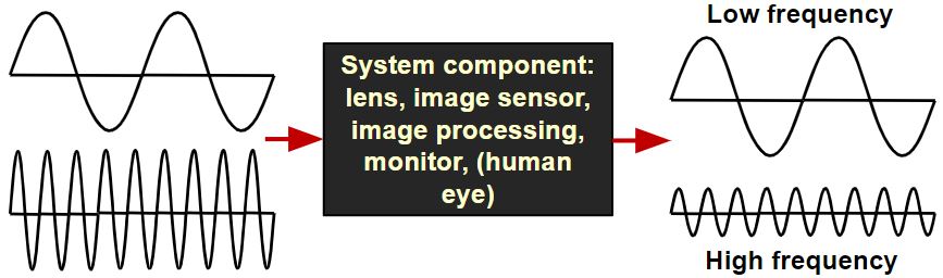
Figure 5. High frequencies correspond to fine detail in the spatial and frequency domains
The relative contrast at a given spatial frequency (output contrast/input contrast) is called Modulation Transfer Function (MTF), which is similar to the Spatial Frequency Response (SFR), and is a key to measuring sharpness. In Figure 6, MTF is illustrated with sine and bar patterns, an amplitude plot, and a contrast plot—each of which has spatial frequencies that increase continuously from left to right.
Note: Imatest uses SFR and MTF interchangeably. SFR is more commonly associated with complete system response, where MTF is commonly associated with the individual effects of a particular component. In other words, system SFR is equivalent to the product of the MTF of each component in the imaging system.
High spatial frequencies (on the right) correspond to fine image detail. The response of photographic components (film, lenses, scanners, etc.) tends to “roll off” at high spatial frequencies. These components can be thought of as low-pass filters that pass low frequencies and attenuate high frequencies.
Figure 6. Sine and bar patterns, amplitude plot, and Contrast (MTF) plot
Figure 6 consists of upper, middle, and lower plots and are described as follows:
- Bar pattern, Sine pattern (upper plot) —The upper plot illustrates (1) the original sine patterns, (2) the sine pattern with lens blur, (3) the original bar pattern, and (4) the bar pattern with lens blur. Note that lens blur causes contrast to drop at high spatial frequencies.
- Amplitude (middle plot)—The middle plot displays the luminance (“modulation” V in the MTF Equation section) of the bar pattern with lens blur (see red curve in Figure 6). The modulation of the sine pattern, which consists of pure frequencies, is used to calculate MTF. (Note that contrast decreases at high spatial frequencies.)
- MTF % (lower plot)—The lower plot shows the corresponding sine pattern contrast (see blue curve; represents MTF), which also is defined in the MTF Equation section. By definition, the low frequency MTF limit is always 1 (100%). In Figure 6, the MTF is 50% at 61 lp/mm (line pairs per millimeter) and 10% at 183 lp/mm. Note that both frequency and MTF are displayed on logarithmic scales with exponential notation [100 = 1%; 101 = 10%; 102 = 100%, etc.]; amplitude (middle plot) is displayed on a linear scale. The MTF of a complete imaging system is the product of the MTF of its individual components.
MTF Equation
The equation for MTF is derived from the sine pattern contrast C(f) at spatial frequency f, where
\(\displaystyle C(f)=\frac{V_{max}-V_{min}}{V_{max}+V_{min}}\) for luminance (“modulation”) V.
\(\displaystyle MTF(f)=100\% \times\frac{C(f)}{C(0)}\) Note: this normalizes MTF to 100% at low spatial frequencies.
To correctly normalize MTF at low spatial frequencies, a test chart must have some low-frequency energy. This is supplied by large light and dark areas in slanted edges and by features in most patterns used by Imatest, but is not present in lines and grids. For systems where sharpening can be controlled, the recommended primary MTF calculation is the slanted-edge, which is calculated from the Fourier transform of the impulse response (i.e., response to a narrow line), which is the derivative (d/dx or d/dy) of the edge response. Fortunately, you don’t need an understanding of Fourier transforms to understand MTF.
Traditional Resolution Measurements
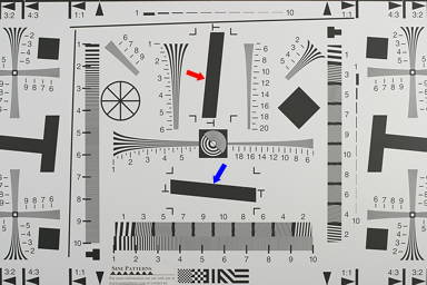
Traditional resolution measurements involve observing an image of bar patterns, most frequently the USAF 1951 chart (Figure 7) and estimating the highest spatial frequency (lp/mm) where bar patterns are visibly distinct. This observation (also called vanishing resolution) corresponds to an MTF of roughly 10-20%. Because the vanishing resolution is the spatial frequency where image information disappears— where it isn’t visible, it is strongly dependent on observer bias and is a poor indicator of image sharpness. (It’s Where the Woozle Wasn’t in Winnie the Pooh.)
Note: The USAF 1951 chart (long-since abandoned by the Air Force) is poorly suited for computer analysis because it uses space inefficiently and its bar triplets lack a low frequency reference. Furthermore, small changes in chart position (sampling phase) can cause the appearance of its bars to change as they shift from being in phase to out of phase with the pixel array. This adversely affects the vanishing resolution estimate.
Figure 7. USAF 1951 chart; not supported by Imatest
Better indicators of image sharpness are spatial frequencies where MTF is 50% of its low frequency value (MTF50) or 50% of its peak value (MTF50P). MTF50 and MTF50P are recommended for comparing the sharpness of different cameras and lenses because
- Image contrast is half its low frequency or peak value thus detail is still quite visible. (The eye is insensitive to detail at spatial frequencies where MTF is 10% or less.)
- The response of most cameras falls off rapidly in the vicinity of MTF50 and MTF50P. MTF50P is a better metric for strongly sharpened cameras (explained in our paper from Electronic Imaging 2020).
- The 50% level is related to the image’s information capacity.
Note: Additional sharpness indicators are discussed in Summary metrics, below.
Although MTF can be estimated directly from images of sine patterns (using Rescharts,Log Frequency, Log F-Contrast, and Star Chart), the ISO 12233 slanted-edge technique provides more accurate and repeatable results and uses space more efficiently. Slanted-edge images can be analyzed by one of the modules listed in the MTF Measurement Matrix, below.
Spatial Frequency Units
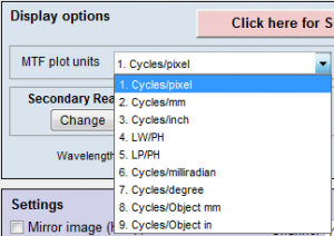
Figure 8. Spatial frequency units are selected in the Settings or More settings windows of SFR and Rescharts modules (SFRplus, eSFR ISO, Star, etc.).
Most readers will be familiar with temporal frequency. For example, the frequency of a sound—measured in Cycles/Second or Hertz—is closely related to its perceived pitch. The frequencies of radio transmissions (measured in kilohertz, megahertz, and gigahertz) are also familiar.
Spatial frequency is measured in cycles (or line pairs) per distance instead of time. As with temporal (e.g., audio) frequency response, the more extended the response, the more detail can be conveyed.
Note: In imaging systems, one cycle (C) is equivalent to one line pair (LP).
The two nomenclatures are used interchangeably.
Spatial frequency units can be selected from the Settings or More settings windows of SFR and Rescharts modules (SFRplus, eSFR ISO, Star, etc. Figure 8) and is the measurement intended to determine how much detail a camera can reproduce or how well the pixels are utilized.
Past film camera lens tests used line pairs per millimeter (lp/mm), which worked well for comparing lenses because most 35mm film cameras have the same 24 x 36mm picture size. But digital sensor sizes vary widely—from under 5mm diagonal in camera phones to 43mm diagonal for full-frame cameras to an even larger diagonal for medium format. For this reason, line widths per picture height (LW/PH) is recommended for measuring the total detail a camera can reproduce. Note that LW/PH is equal to 2 × lp/mm × (picture height in mm).
Another useful spatial frequency unit is cycles per pixel (C/P), which gives an indication of how well individual pixels are utilized. The choice of units is also influenced by whether performance at the image (sensor) or on the object has primary importance: see Comparing sharpness in different cameras. There is no need to use actual distances (millimeters or inches) with digital cameras, although such measurements are available (Table 1).
Table 1. Summary of spatial frequency units with equations that refer to MTF in selected frequency units.
| MTF Unit | Application | Equation |
|
Cycles/Pixel (C/P) |
Shows how well pixels are utilized. Nyquist frequency fNyq is always 0.5 C/P. |
|
|
Cycles/Distance (cycles/mm or cycles/inch) |
Cycles per distance on the sensor. Pixel spacing or pitch must be entered. Popular for comparing resolution in the old days of standard film formats (e.g., 24x36mm for 35mm film). |
\(\frac{MTF(C/P)}{\text{pixel pitch}}\) |
|
Line Widths/Picture Height (LW/PH) note: for cropped images enter the original picture height into the more settings dimensions input |
Measures overall image sharpness. This is the best unit for comparing the performance of cameras with different sensor sizes and pixel counts. Line Widths is traditional for TV measurements. Recommended for image-centric applications in Comparing sharpness in different cameras. Note that 1 Cycle = 1 Line Pair (LP) = 2 Line Widths (LW). |
\(2 \times MTF\bigl(\frac{LP}{PH}\bigr)\) ; \(2 \times MTF\bigl(\frac{C}{P}\bigr) \times PH\) |
|
Line Pairs/Picture Height (LP/PH) note: for cropped images enter the original picture height into the more settings dimensions input |
Measures overall image sharpness. Differs from LW/PH by a factor of 2. Used by dpreview.com. |
\(MTF\bigl(\frac{LW}{PH}\bigr) / 2\) ; \(MTF\bigl(\frac{C}{P}\bigr) \times PH\) |
|
Angular frequency Cycles/milliradian |
Angular frequencies. Pixel spacing or pitch must be entered. Focal length (FL) in mm is usually included in EXIF data in commercial image files. If it isn’t available it must be entered manually, typically in the EXIF parameters region at the bottom of the settings window. If pixel spacing or focal length is missing, units will default to Cycles/Pixel. FL can be calculated from the simple lens equation*, \(1/FL = 1/s_1 + 1/s_2\), where s1 is the lens-to-chart distance (easy to measure), s2 is the lens-to-sensor distance, and magnification \(M = s_2/s_1\). \(FL = s_1/(1+1/|M|)\ =\ s_2/(1+|M|)\) *Unless s1 >> s2, (by 100× or more), lens geometry (s1, s2, and FL) is not reliable for calculating M because lenses can deviate significantly from the simple lens equation. |
\(0.001 \times MTF\bigl(\frac{\text{cycles}}{\text{mm}}\bigr) \times FL(\text{mm})\) |
|
Cycles/degree |
\(\frac{\pi}{180} \times MTF\bigl(\frac{\text{cycles}}{\text{mm}}\bigr) \times FL(\text{mm})\) |
|
|
Cycles/object mm Measured on the object being photographed, not on the image sensor. |
Cycles per distance on the object being photographed (what some people think of as the “subject”).
For object-centric applications see Comparing sharpness in different cameras. |
\(MTF\bigl( \frac{\text{Cycles}}{\text{Distance}} \bigr) \times |\text{Magnification}|\) Distance can be mm or inches. Pixel spacing (pitch) is not required for eSFR ISO, SFRplus, and Checkerboard. Cycles/object distance is Cycles/mm or Cycles/in on the object being photographed. |
|
Line Widths/Crop Height |
Primarily used for testing when the active chart height (rather than the total image height) is significant. No longer recommended because it’s dependent on the crop size, which is not standardized. | |
|
Line Widths/ (formerly Line Widths or Line Pairs/N Pixels (PH)) |
When either of these is selected, a Feature Ht pixels box appears to the right of the MTF plot units (sometimes used for Magnification) that lets you enter a feature height in pixels, which could be the height of a monitor under test, a test chart, or the active field of view in an image that has an inactive area. This unit selection is useful for comparing the resolution of specific objects for cameras with different image or pixel sizes. Recommended for object-centric applications in Comparing sharpness in different cameras. |
\(2 \times MTF\bigl(\frac{C}{P}\bigr) \times \text{Feature Height}\) \(MTF\bigl(\frac{C}{P}\bigr) \times \text{Feature Height}\) |
|
PH = Picture Height in pixels. FL(mm) = Lens focal length in mm. Pixel pitch = distance per pixel = 1/(pixels per distance). |
||
Comparing sharpness in different cameras recommends spatial frequency units based on one of two broad types of application:
-
- Image-centric (such as landscape photography, where detail on the image sensor is important): Line Widths (or Pairs) per Picture Height is recommended.
- Object-centric (for medical, machine vision, etc., where details of the object are important): Cycles/object distance or LW (or LP) per Feature Height are recommended.
Summary Metrics
Several summary metrics are derived from MTF curves to characterize overall performance. These metrics are used in a number of displays, including secondary readouts in the SFR/SFRplus/eSFR ISO Edge/MTF plot (see Imatest Slanted-Edge Results) and in the SFRplus 3D maps.
| Summary Metric | Description | Comments |
| MTF50 MTFnn |
Spatial frequency where MTF is 50% (nn%) of the low (0) frequency MTF. MTF50 (nn = 50) is widely used because it corresponds to bandwidth (the half-power frequency) in electrical engineering. | The most common summary metric; correlates well with perceived sharpness. Increases with increasing software sharpening; may be misleading because it “rewards” excessive sharpening, which results in visible and possibly annoying “halos” at edges. |
| MTF50P MTFnnP |
Spatial frequency where MTF is 50% (nn%) of the peak MTF. | Identical to MTF50 for low to moderate software sharpening, but lower than MTF50 when there is a software sharpening peak (maximum MTF > 1). Much less sensitive to software sharpening than MTF50 (as shown in a paper we presented at Electronic Imaging 2020). All in all, a better metric. |
| MTF area normalized |
Area under an MTF curve (below the Nyquist frequency), normalized to its peak value (1 at f = 0 when there is little or no sharpening, but the peak may be » 1 for strong sharpening). | A particularly interesting new metric because it closely tracks MTF50 for little or no sharpening, but does not increase for strong oversharpening; i.e., it does not reward excessive sharpening. Still relatively unfamiliar. Described in Slanted-Edge MTF measurement consistency. |
| MTF10, MTF10P, MTF20, MTF20P |
Spatial frequencies where MTF is 10 or 20% of the zero frequency or peak MTF | These numbers are of interest because they are comparable to the “vanishing resolution” (Rayleigh limit). Noise can strongly affect results at the 10% levels or lower. MTF20 (or MTF20P) in Line Widths per Picture Height (LW/PH) is closest to analog TV Lines. Details on measuring monitor TV lines are found here. |
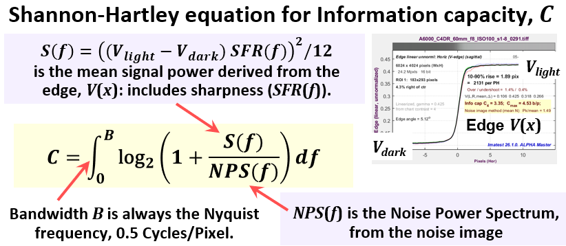
| Shannon information capacity | Not strictly a sharpness metric! Combines MTF, noise, and contrast loss to give a figure of merit for imaging systems.. | Can be measured from Siemens Star or Slanted-edge patterns. Slanted-edges are faster and more convenient. Sensitive to exposure level. New and still unfamiliar: we are making an effort to educate the industry about its merits. Details and news on Image Information Metrics: Information Capacity and more. |
MTF Measurement Matrix — comparing different charts and measurement techniques
Imatest has many patterns for measuring MTF— slanted-edge, Log frequency, Log f-contrast, Siemens Star, Dead Leaves (Spilled Coins), Random 1/f, and Hyperbolic wedge— each of which tends to give different results in consumer cameras, most of which have nonuniform image processing— commonly bilateral filtering— that depends on local scene content. Sharpening (high frequency boost) tends to be maximum near contrasty features (larger near higher contrast edges), while noise reduction (high frequency cut, which can obscure fine texture) tends to be maximum in their absence. For this reason MTF measurements can be very different with different test charts.
In principle, MTF measurements should be the same when no nonuniform or nonlinear image processing (bilateral filtering) is applied, for example when the image is demosaiced with dcraw or LibRaw with no sharpening and noise reduction. But this does not exactly happen because demosaicing, which is present in all cameras that use Color Filter Arrays (CFAs) involves some nonlinear processing. The sensitivity of different patterns to image processing is summarized in the image below.
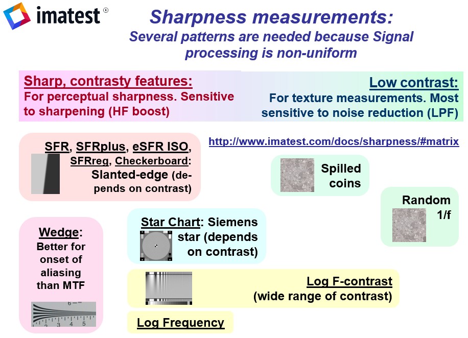 Comparison of the effects of image processing (bilateral filtering) on MTF measurements:
Slanted-edges and wedges tend to be sharpened the most.
The random 1/f pattern has the least sharpening and the most noise reduction.
The MTF Matrix table below lists the attributes, advantages, and disadvantages of Imatest’s methods for measuring MTF.
MTF Measurement Matrix
| Measurement pattern |
Advantages / Disadvantages / Sensitivity | Primary use & comments |
| Slanted-edge (SFR SFRplus eSFRiso SFRreg Checkerboard) |
Most efficient use of space: enables creation of a detailed map of MTF response. Fast, automated region detection in SFRplus, eSFR ISO, SFRreg, and Checkerboard. Fast calculations. Relatively insensitive to noise (more immune if noise reduction is applied). Compliant with the ISO 12233 standard, using a “binning” (super-resolution) algorithm that allows MTF to be measured above the Nyquist frequency (0.5 C/P). The best pattern for manufacturing testing. May give optimistic results in systems with strong sharpening and noise reduction (i.e., it can be fooled by signal processing, especially with high contrast (≥ 10:1) edges. Gives inconsistent results in systems with extreme aliasing (strong energy above the Nyquist frequency), especially with small regions. Most sensitive to sharpening, especially for high contrast (≥10:1) edges; Least sensitive to software noise reduction. |
This is the primary MTF measurement in Imatest. The most efficient pattern for lens and camera testing, especially where an MTF response map is required. The high contrast (≥40:1) recommended in the old ISO 12233:2000 standard produced unreliable results (clipping, gamma issues, excessive sharpening with bilateral filters). The new ISO 12233:2014 standard recommends 4:1 contrast. This is our recommendation (with SFRplus or eSFR ISO) for all new work. Compared favorably with the Siemens star in Slanted-edge versus Siemens Star. |
| Log frequency | Calculated from first principles. Displays color moire. Sensitive to noise. Inefficient use of space. |
Primarily used as a check on other methods, which are not calculated from first principles. |
| Log f-Contrast | Best pattern for illustrating the effects of nonuniform image processing. Sensitive to noise. Strong sensitivity to sharpening near the (high contrast) top of the image and noise reduction near the (low contrast) bottom, with a gradual transition in-between. |
The sensitivity to sharpening/noise reduction is an advantage for this chart, which is designed to Illustrate how signal processing varies with image content (feature contrast). Shows loss of fine detail due to software noise reduction. |
| Siemens star | Included in the ISO 12233:2014 standard. Relatively insensitive to noise. Provides directional MTF information. Slow, inefficient use of space. Limited low frequency information at outer radius makes MTF normalization difficult. Moderate sensitivity to sharpening and noise reduction. |
Promoted for general testing by Image Engineering, but spatial detail is limited to a 3×3 or 4×3 grid. Compared with the slanted-edge in Slanted edge vs. Siemens star MTF calculations: 2024 white paper. |
| Dead Leaves (Spilled Coins) |
Measures texture blur / sharpness / acutance. Pattern statistics are similar to typical images. Inefficient use of space. A tricky noise power subtraction algorithm* can reduce very high sensitivity to noise, but signal-averaging of multiple identical images works better. Moderate sensitivity to sharpening and strong sensitivity to noise reduction make it usable for an overall texture sharpness metric that correlates well with subjective observations. |
Consists of stacked randomly-sized circles. Strong industry interest, particularly from the Camera Phone Image Quality (CPIQ) group.
Both Dead Leaves (Spilled Coins) and Random charts are analyzed with the Random (Dead Leaves) module. Strong bilateral filtering can cause misleading results. |
| Random (scale-invariant) | Reveals how well fine detail (texture) is rendered: system response to software noise reduction. Lest sensitive to sharpening, Most sensitive to Software noise reduction |
Measures a camera’s ability to render fine detail (texture), i.e., low contrast, high spatial frequency image content. *Noise power can be removed from the measurement in Imatest using the gray patches adjacent to the pattern. |
| Wedge | Makes use of wedge patterns on the ISO 12233:2000 or eSFR ISO chart. MTF is not accurate around Nyquist and half-Nyquist frequencies (it’s very sensitive to sampling phase variations). Not suitable as a primary MTF measurement. Sensitive to sharpening. Sensitive to noise. Inefficient use of space. |
Measures “vanishing resolution”: where lines start disappearing in wedge patterns, frequently in the ISO 12233 chart, where three regions (including a square region for a low-frequency reference) are required to get a reasonable MTF measurement (which is less accurate than other methods due to sampling phase sensitivity). More convenient with eSFR ISO. |
| The effects of noise (and low Signal-to-Noise Ratio – SNR) can be greatly reduced by acquiring and signal-averaging multiple images. |
||
Slanted-Edge Measurement for Spatial Frequency Response
Several Imatest modules measure MTF using the slanted-edge technique and include:
- Slanted-edge test charts that may be purchased from Imatest or created with Imatest Test Charts. Charts that employ automatic detection (SFRplus, eSFR ISO, SFRreg, or Checkerboard) are recommended.
- Briefly, the ISO 12233 slanted-edge method calculates MTF by finding the average edge (4X oversampled using a clever binning algorithm), differentiating it (to obtain the Line Spread Function (LSF)), and taking the absolute value of the Fourier transform of the LSF. The algorithm is described in detail here.
The key output of slanted edge analysis is the Edge/MTF plot, which can be viewed by clicking the button below. Many additional results are available, including summary and 3D plots, showing Lateral Chromatic Aberration and other results as well as MTF.
The Edge/MTF plot: Imatest’s primary slanted-edge result
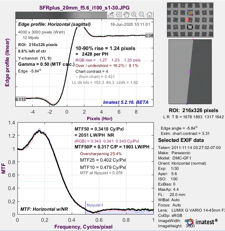 An Edge/MTF plot from Imatest SFR (for an SFRplus chart image) is shown on the right. SFRplus, eSFR ISO, SFRreg, and Checkerboard produce similar results and much more.
(Upper-left) A narrow image illustrating the tones of the averaged edge. It is aligned with the average edge profile (spatial domain) plot, immediately below.
(Middle-left) Average Edge (Spatial domain): The average edge profile shown here linearized (the default). A key result is the edge rise distance (10-90%), shown in pixels and in the number of rise distances per Picture Height. Other parameters include overshoot and undershoot (if applicable). This plot can optionally display the line spread function (LSF: the derivative of the edge).
(Bottom-left) MTF (Frequency domain): The Spatial Frequency Response (MTF), shown to twice the Nyquist frequency. Key summary results include MTF50, the frequency where contrast falls to 50% of its low frequency value, and MTF50P, the frequency where contrast falls to 50% of its peak value, which corresponds well with perceived image sharpness. Units are cycles per pixel (C/P) and Line Widths per Picture Height (LW/PH). Other results include MTF at Nyquist (0.5 cycles/pixel; sampling rate/2), which indicates the probable severity of aliasing and user-selected secondary readouts, and Secondary readouts. The Nyquist frequency is displayed as a vertical blue line. The diffraction-limited MTF response is shown as a pale brown dashed line when the pixel spacing is entered (manually) and the lens focal length is entered (usually from EXIF data, but can be manually entered).
This image is strongly (but not excessively) sharpened.
SFR Results: MTF (sharpness) plot describes this Figure in more detail.
MTF curves and Image appearance contains several examples illustrating the correlation between MTF curves and perceived sharpness.
Why is the edge slanted?
MTF results for pure vertical or horizontal edges are highly dependent on sampling phase (the relationship between the edge and the pixel locations), and hence can vary from one run to the next depending on the precise (sub-pixel) edge position. The edge is slanted so MTF is calculated from the average of many sampling phases, which makes results much more stable and robust (Figure 9).
What edge angles work best?
Where possible, edge angles should be greater than ±2 degrees from the closest Vertical (V), Horizontal (H), or 45 degree orientation. The reason is that results from vertical, horizontal, and 45° edges are very sensitive to the relationship between the edge and the pixels (i.e., they are phase-sensitive). Tilting the edges by more than 2 or 3 degrees avoids this issue.
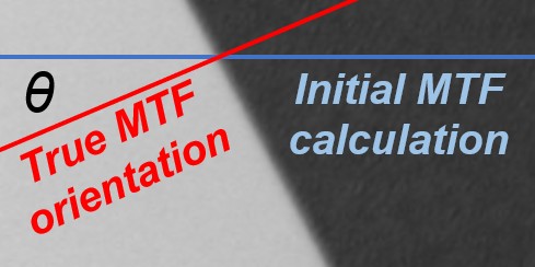 The ISO 12233 standard recommends an angle of either 5 or 5.71 degrees (arctan(0.1)). This angle is not sacred— MTF is not strongly dependent on edge angle. Angles from 3 to 7 degrees work fine. For nonzero edge angles θ relative to the closest V or H orientation, a cosine correction is applied, as illustrated on the right. The correction is significant when θ is greater than about 8 degrees (cos(8º) = 0.99). The initial MTF and corresponding frequency f are calculated from a Vertical or Horizontal line (shown in blue), based on the region selection. The true MTF is defined normal to the edge— along the red line. Since the length of the actual transition along the red line (normal to the edge) is shorter than the measured transition along the blue (V or H) line, and since the frequency f used to measure MTF is inversely proportional to the actual transition length,
\(f=f_{initial} / cos(\theta)\)
Corresponding summary metrics MTFnn (MTF50, MTF50P, etc.), which have units of frequency, are increased over the initial values.
\(MTFnn = MTFnn(\text{initial}) / cos(\theta)\)
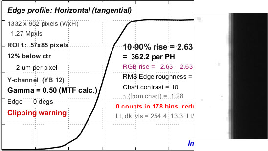
Clipped high-contrast vertical edge (results are not valid)
The primary disadvantage of large edge angles is that the available region area may be reduced, especially for SFRreg patterns.
Edge Contrast and clipping
Edge Contrast should be limited to 10:1 at the most, and a 4:1 edge contrast is generally recommended. The reason is that high contrast edges (>10:1, such as found in the old ISO 12233:2000 chart) can cause saturation or clipping, resulting in edges with sharp corners that exaggerate MTF measurements. For more details, see Using Rescharts slanted-edge modules, Part 2: Warnings – clipping.
Advantages and Disadvantages of the Slanted Edge
Advantages
- Most efficient use of space, which makes it possible to create a detailed map of MTF response
- Fast, automated region detection in SFRplus, eSFR ISO, SFRreg, and Checkerboard
- Fast calculations
- Relatively insensitive to noise (highly immune if noise reduction is applied)
- Compliant with the ISO 12233 standard, whose “binning” (super-resolution) algorithm allows MTF to be measured above the Nyquist frequency (0.5 C/P)
- The best pattern for manufacturing testing
Disadvantages
- May give optimistic results in systems with strong image-dependent sharpening (i.e., where the amount of sharpening increases with edge contrast). This type of image processing (bilateral filtering) is almost universal in consumer cameras.
- Gives inconsistent results in systems with extreme aliasing (strong energy above the Nyquist frequency), especially with small regions.
- Not suitable for measuring fine texture, where the Log Frequency-Contrast or Spilled Coins (Dead Leaves) patterns are recommended.
Note: Imatest Master can calculate MTF for edges of virtually any angle, though exact vertical, horizontal, and 45° should be avoided because of sampling phase sensitivity.
Slanted-Edge Modules
Imatest Slanted-Edge Modules include SFR, SFRplus, eSFR ISO, Checkerboard, and SFRreg (see Table 2 and Sharpness Modules for details).
Note: See “How to test lenses with Imatest” for a good summary of how to measure MTF using SFRplus or eSFR ISO.
Table 2. Brief summary of Imatest slanted-edge modules.
| Module | Description | Examples |
|---|---|---|
| SFR |
|  |
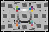
| SFRplus |
|  |
| eSFR ISO |
|  |
| Checkerboard |
| 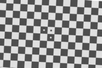 |
| SFRreg | Several individual charts are typically placed around the image field; works with:
| 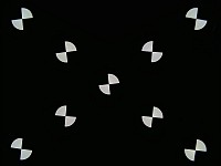 |
Slanted-Edge Algorithm
The MTF calculation is derived from ISO standard 12233. The Imatest calculation contains a number of enhancements, listed below. The original ISO calculation is performed when the ISO standard SFR checkbox in the SFR input dialog box is checked (we recommended leaving it unchecked unless it’s specifically required).
- The cropped image is linearized; i.e., the pixel levels are adjusted to remove the gamma encoding applied by the camera. (Gamma is adjustable with a default of 0.5).
- The edge locations for the red, green, blue, and luminance (Y) channels are determined for each scan line (horizontal lines in the above image).
- A second order fit to the edge is calculated for each channel using polynomial regression. The second order fit removes the effects of lens distortion. In the above image, the equation would have the form:
\(x = a_0 + a_1y + a_2y^2\)
- Depending on the value of the fractional part of scan line i,
fp = xi – int(xi )
of the second order fit at each scan line, the shifted edge is added to one of four bins:
bin 1 if 0 ≤ fp < 0.25
bin 2 if 0.25 ≤ fp < 0.5
bin 3 if 0.5 ≤ fp < 0.75
bin 4 if 0.75 ≤ fp < 1
Note: The bin mentioned in the previous equation does not depend on the detected edge location.
-
- The four bins are combined to calculate an averaged 4x oversampled edge. This allows analysis of spatial frequencies beyond the normal Nyquist frequency.
- The derivative (d/dx) of the averaged 4x oversampled edge is calculated. A centered Hamming window is applied to force the derivative to zero at its limits.
- MTF is the absolute value of the Fourier transform (FFT) of the windowed derivative.
- The four bins are combined to calculate an averaged 4x oversampled edge. This allows analysis of spatial frequencies beyond the normal Nyquist frequency.
Note: Origins of Imatest slanted-edge SFR calculations were adapted from a Matlab program, sfrmat, which was written by Peter Burns to implement the ISO 12233:2000 standard. Imatest’s SFR calculation incorporates numerous improvements, including improved edge detection, better handling of lens distortion, and better noise immunity. The original Matlab code is available here. In comparing sfrmat results with Imatest, tonal response is assumed to be linear; i.e., gamma = 1 if no OECF (tonal response curve) file is entered into sfrmat. Since the default value of gamma in Imatest is 0.5, which is typical of digital cameras in standard color spaces such as sRGB, you must set gamma to 1 to obtain good agreement with sfrmat.
Imatest and ISO Standard 12233 calculation options
New in Version 22.1 – an Imatest/ISO Standard SFR dropdown menu is located on the lower left of slanted-edge More Settings window. (This option was formerly a checkbox for “ISO compatible” calculations),
This new dropdown allows you to choose between Imatest and ISO-compliant calculations. There are now four options that can be used for SFR Settings to control the Edge SFR Algorithm.
- Imatest pre-22.1 – this option maintains the pre-22.1 Imatest SFR calculations, which are based on ISO 12233:2017, with 3rd order polynomial curved edge fitting, LSF Correction Factor and a correction factor for the angle of the edge.
- ISO 12233:2017 & earlier – implements the 12233:2017 algorithm with Hamming window and linear edge fitting.
- Imatest 22.1 (recommended) – Our recommended calculation, based on the ISO 12233:2024 standard, but with a lowpass filter use to locate the edge which makes it function in noisier images. Uses the Tukey window (alpha=1), 5th order polynomial edge fitting, LSF Correction Factor and a correction factor for the angle of the edge
- ISO 12233:2024 – implements the current 12233:2024 algorithm, uses a centroid to detect the edge which is sensitive to noise. Uses the Tukey window (alpha=1), 5th order polynomial edge fitting, LSF Correction Factor and a correction factor for the angle of the edge
Differences Between the Imatest calculations and standard ISO 12233 Calculations
Setting #2 (ISO 12233 2017 & earlier) is not recommended because the Imatest and newer ISO calculations are more accurate— definitely superior in the presence of noise and optical distortion. More information on calculations can be found below:
- The center of each scan line is calculated from the peak of the lowpass-filtered edge derivative in the Imatestcalculations. The ISO calculation uses a centroid, which is optimum in the absence of noise. But noise is always present to some degree, and the centroid is extremely sensitive to noise because noise at large distances from the edge has the same weight as the edge itself. The lowpass-filter is closer to a matched filter, which optimally detects the edge derivative peak.
- Gamma(used to linearize the data) is entered as an input value or derived from known chart contrast. In ISO-standard implementations it is assumed to be 1 unless an OECF file is entered.
- Imatest assumes that the edge may have some (second-order) curvature due to optical distortion. ISO-standard calculation through 2017 assumes a straight line, which can result in degraded MTF measurements in the presence of optical distortion. Curved edges (5th order fit) are included in the ISO 12233:2022+ calculation. There is very little difference with the 2nd order fit of the older Imatest calculation.
- Imatest’s “modified apodization” noise reduction (on by default) results in more consistent measurements (no systematic difference). It is turned off when the ISO standard calculation is checked
- The Line Spread Function (LSF) correction factor, introduced in ISO 12233:2014 has been implemented in Imatestsince 2015. The correction factor D(j) (or D(k)), which compensates for the high frequency loss from numerical differentiation when calculating LSF from the Edge Spread Function (ESF), is incorrect in both the ISO 12233:2014 and 2017 standards. The Imatest and newer ISO implementation, which is based on first principles (we have the full set of equations), complies with the intent of both versions of the standard.
- A Tukey window is used in the newer Imatest and ISO calculations. It seems to make very little difference.
Note that Additional calculation details can be found in the Peter Burns links (below)
Key Takeaways
- Frequency and spatial domain plots convey similar information, but in a different form. A narrow edge in spatial domain corresponds to a broad spectrum in frequency domain (extended frequency response) and vice-versa.
- Imatest measures the system response, which includes image processing: not just the lens response.
- Sensor response above the Nyquist frequency can cause aliasing that is visible as Moiré patterns of low spatial frequency. In Bayer sensors (all sensors except Foveon), Moiré patterns appear as color fringes. Moiré in Foveon sensors is far less bothersome because it is monochrome and the effective Nyquist frequency of the Red and Blue channels is lower than with Bayer sensors.
- MTF at and above the Nyquist frequency is not an unambiguous indicator of aliasing problems. MTF is the product of the lens and sensor response, demosaicing algorithm, and sharpening that frequently boosts MTF at the Nyquist frequency. MTF should be interpreted as a warning that there could be problems.
- Results are calculated for the R, G, B, and Luminance (Y) channels. The Y channel is normally displayed in the foreground, but any of the other channels can selected. All are included in the .CSV output file.
- Horizontal and vertical resolution can be different for CCD sensors and should be measured separately. They’re nearly identical for CMOS sensors. Recall, horizontal resolution is measured with a vertical edge and vertical resolution is measured with a horizontal edge. Resolution is only one of many criteria that contributes to image quality.
- MTF can vary throughout the image, and it doesn’t always follow the expected pattern of sharpest near the center and less sharp near the corners. There are any number of reasons: lens misalignment, curvature of field, misfocus, etc. That is why measurements are important.
See Also
- Imatest Knowledge Base: Sharpness
- Diffraction, Optimum Aperture, and Defocus
- Slanted Edge Noise Reduction (Modified Apodization Technique)
Additional Resources
- Calibration Targets (Google Earth Blog) Calibration targets – mostly for MTF – visible from satellites. Part 5. Around the world, is particularly interesting. A customer has used a target in 13300 Salon-de-Provence, France.
- Diagnostics for Digital Capture using MTF by Don Williams and Peter D. Burns (2001), Applying and Extending ISO/TC42 Digital Camera Resolution Standards to Mobile Imaging Products by Don Williams and Peter D. Burns (2007) (Contains an image of the low-contrast slanted-edge test chart proposed for the revised ISO 12233 standard.)
- How to Read MTF Curves by H. H. Nasse of Carl Zeiss. Excellent, thorough introduction. 33 pages long; requires patience. Has a lot of detail on the MTF curves similar to the Lens-style MTF curve in SFRplus. Even more detail in Part II.
- Slanted-Edge MTF for Digital Camera and Scanner Analysis by Peter D. Burns (2000) (alternate source). An excellent introduction to the ISO 12233 slanted-edge measurement. Closely related: Diagnostics for Digital Capture using MTFby Don Williams and Peter D. Burns (2001), Applying and Extending ISO/TC42 Digital Camera Resolution Standards to Mobile Imaging Products by Don Williams and Peter D. Burns (2007) (Contains an image of the low-contrast slanted-edge test chart proposed for the revised ISO 12233 standard.
