From the Imatest main window, click on or on the upper left. SFR allows you to analyze multiple regions and to run batches of files. Rescharts (1. Slanted-edge SFR) allows you to analyze single regions in a highly-interactive interface.
ISO 12233:2000 chart images, which have contrasty (≥40:1) slanted-edges, can be downloaded from dpreview.com reviews, typically in the last page titled “Compared to…,” and from Imaging-resource.com reviews, typically on the page labeled “sample images.” We no longer recommend such high contrast images, because saturation can lead to inaccurate results. 4:1 or 10:1 contrast images are much preferred.
Image file – ROI – Cropping recommendations (ROI size) – Additional SFR settings – Secondary Readout
Equations – Gamma – Warnings – Saving – Repeated runs – Excel CSV output
Selecting the image file (or batches of files)
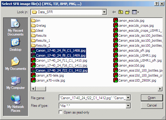
When you click from the Imatest main window or (with Rescharts Slanted-edge SFR selected), the window below appears, requesting the image file name(s). The folder saved from the previous run appears in the Look in: box on the top. You are free to change it. You can open a single file by simply double-clicking on it. You can select multiple files (for batch mode or combined runs with SFR in Imatest Master or Image Sensor) by the usual Windows techniques: control-click to add a file; shift-click to select a block of files. Then click . Three image files are highlighted below. Large files can take several seconds to load. Imatest remembers the last folder used (for each module, individually). In batch mode the first file is handled like a normal run; the remaining files run in express mode (no settings windows).
File selection
If the folder contains meaningless camera-generated file names such as IMG_3734.jpg, IMG_3735.jpg, etc., you can change them to meaningful names that include focal length, aperture, etc., with the Rename Files utility, which takes advantage of EXIF data stored in each file.
|
| RAW files Imatest SFR can analyze Bayer raw files: standard files (TIFF, etc.) that contain undemosaiced data. RAW files have limited value for measuring MTF because the pixel spacing in each image planes is twice that of the image as a whole; hence MTF is lower than for demosaiced files. But Chromatic aberration can be severely distorted by demosaicing (and can be fixed prior to demosaicing), and is best measured in Bayer RAW files (and corrected during RAW conversion). Details of RAW files can be found here. |
Selecting the ROI (Region of Interest)
Imatest SFR can analyze slanted edges of almost any angle from any source, though angles between 2 and 7 degrees with respect to horizontal or vertical are recommended. Larger angles are OK (a cosine correction is automatically applied). Pure horizontal, vertical, or 45 degree edges should be avoided. The images can come from the environment as well as from test charts. For best results, contrast should not be too high. The ISO 12233:2000 chart, shown below, has excessive contrast (≥40:1), which can lead to errors from saturation/clipping. Contrast ratios between 10:1 and 2:1 (used in SFRplus and eSFR ISO charts) are recommended. 4:1 is specified in the ISO 12233/2014/2017 standard.
If the image has the same pixel dimensions as the image in the previous run, a dialog box shown below asks you if you want to repeat the same ROIs (regions of interest) as the previous image. If you answer No or if the image has a different size, the coarse selection dialog box shown below is opened. Select ROI by clicking and dragging, or clicking outside image. Click on one corner of the intended region, drag the mouse to the other corner, then release the mouse button. Click outside the image or on the Select entire image button to select the entire image.
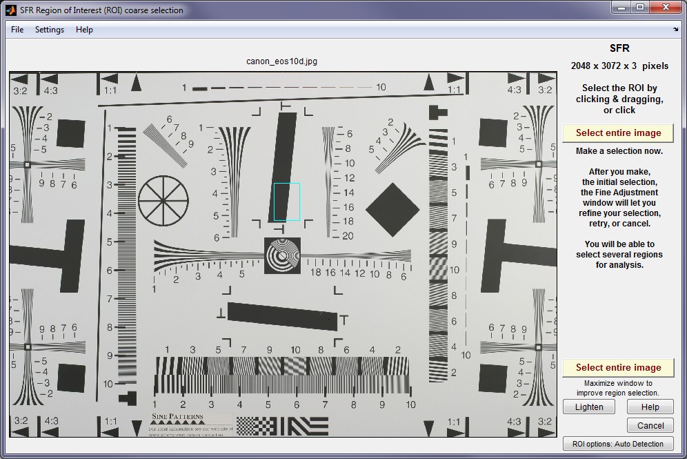 ROI selection: ISO 12233:2000 chart
Note: the Zoom feature of Matlab Figures  does not work here. Imatest mistakenly assumes you are trying to select the entire image. To enlarge the image (to view the crop area more clearly), maximize it by clicking on the square near the upper right corner.
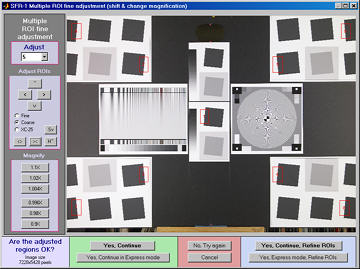
After you make your selection the ROI fine adjustment dialog box, shown below, appears. You can move the entire ROI or any of the edges in increments of one pixel. You can also enter the ROI boundary locations in the boxes below the image. If you do this, be sure to press return (or move the cursor) to register the change. You can zoom out to view the entire image, then zoom back in. The ROI fine adjustment is particularly valuable for maximizing the size of small regions and excluding interfering detail.
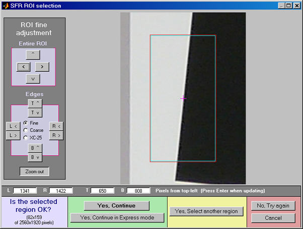
ROI fine adjustment
When you finish adjusting the ROI, proceed by selecting one of five choices at the bottom of the box.
| Yes, Continue | The selected ROI is correct; no more ROIs are to be selected. Continue with SFR calculations in normal mode: You will be asked for additional input data, if required. |
| Yes, Continue in Express mode | The selected ROI is correct; no more ROIs are to be selected. Continue with SFR calculations in Express mode: You will not be asked for additional input data or for Save options. Saved or default settings will be used. |
| Yes, select another region | Accept the selected RO, and select another. |
| No, try again | The selected ROI is not correct. Try again. |
| Cancel | Cancel the SFR run. Return to the Imatest main window. |
If the the height or width of the ROI is under 10 pixels, the ROI is over 1,000,000 (500,000 for strong filtering) pixels or appears to be inappropriate, you’ll be asked to repeat the selection. The ROI is normally checked for validity, but there are some cases (e.g., endoscopes) where valid images may fail the usual tests ROI filtering can be relaxed considerably by opening the button in the Imatest main window (Master-only) and clicking Light filtering in the first group of controls. This can can lead to errors when regions are selected carelessly. Normal filtering is the default.
ROI settings are saved after the run is complete. You can save these particular ROIs for future runs in a named file by clicking on Save settings… in the INI File Settings dropdown menu in the Imatest main window. These settings can be retrieved later by clicking on Load settings.
Cropping recommendations (ROI size)
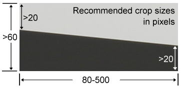
For best accuracy the length (dimension along the edge) should be between 80 and 500 pixels and the width (dimension normal to the edge) should be at least half the length. Little is gained for lengths over 300 pixels.* The absolute crop limits are 10 and 2000 pixels (1400 maximum for strong filtering). Typical crops for medium-high resolution images are between around 120x80 and 300x140 pixels.
For small, low resolution images, we recommend a minimum of 40×25 pixels, If possible. Minimum widths for light and dark zones should be at least 8 pixels, with 20 preferred (shown on the right). Little is gained for minimum dark/light zone widths over 50 pixels or total width over 100 pixels.
MTF results are insensitive to crop size, though smaller crops are more sensitive to variations due to noise. The relationship between MTF, crop size, and noise is described in Slanted-edge MTF measurement consistency.
For very small crops (width or length between 10 and about 25 pixels) a warning message may appear in place of the light/dark level display: Zero counts in n bins. Accuracy may be reduced. This indicates that some interpolation was required to obtain the final results, which may not be as accurate or repeatable as they would be for larger ROIs.
Small crops or noisy images may require weaker error filtering than normal crops/images. Press in the Imatest main window and set SFR ROI filtering to None or Light.
Saving ROIs between runs. ROIs may be saved in named files by clicking on the INI File Settings dropdown menu, then pressing Save ROI settings…. To restore the saved settings, click on the Load (merge) ROI settings…. This allows you to recover saved ROIs after runs with different image sizes and ROIs. (The most recent settings are automatically saved and loaded: this is for long-term use.) Note that Save settings… and Load settings… save and load all settings, not just ROIs.
*An exception is when the MTF of inkjet test charts is measured, as described in Compensating camera MTF measurements for chart and sensor MTF. Inkjet charts are quite rough and may require large regions for good results.
SFR settings window
The Imatest SFR settings window, shown below, opens after the Region of Interest (ROI) has been selected, unless Express mode has been selected. It appears only once during multiple ROI runs. Succeeding runs use the same settings except for (calculated) Crop location. All input fields are optional. Most of the time you can simply click (the button on the lower right) to continue.
 SFR input dialog box
This window is divided into sections: Title and on top, then Display Options, Plot, Settings, Optional parameters, and finally, or .
Title defaults to the input file name. You may leave it unchanged, replace it, or add descriptive information for the camera, lens, converter settings, etc.— as you please.
opens a browser window containing a web page describing the module.
Plot
Select results to plot. Edge/MTF and Chromatic Aberration are shown checked.
Edge/MTF is the primary results plot, showing the average edge and MTF response. The MTF plot units dropdown menu in Display options selects MTF spatial frequency units: 1. Cycles/pixel, 2. Cycles/mm, 3. Cycles/inch, 4. LW/PH (Line Widths per Picture Height), 5. LP/PH (Line Pairs per Picture Height), 6. Cycles/milliradian, 7. Cycles/degree can be selected, 8. Cycles/object mm, 9. Cycles/object in, and more. If 2, 3, or 6-9 are selected, the pixel size should be entered in the box immediately below with the appropriate units (pixels per inch, pixels per mm, or microns per pixel) selected in the dropdown menu to the right. If pixel size is omitted, the x-axis will be displayed in the default units, Cycles per pixel..
| Pixel size has an important relationship to image quality. For very small pixels, noise, dynamic range and low light performance suffer. Pixel size is rarely given in spec sheets: it usually takes some math to find it. If the sensor type and the number of horizontal and vertical pixels (H and V) are available, you can find pixel size from the table on the right and the following equations. pixel size in mm = (diagonal in mm) / sqrt(H2+V2) pixel size in microns = 1000 (diagonal in mm) / sqrt(H2+V2)Pixel size in microns (microns per pixel) can be entered directly into the SFR input dialog box. Example, the 5 megapixel Panasonic Lumix DMC-TZ1 has a 1/2.5 inch sensor and a maximum resolution of 2560×1980 pixels. Guessing that the diagonal is 7 mm, pixel size is 2.1875 (rounded, 2.2) microns.You can find detailed sensor specifications in pages from Sony, Panasonic, and Kodak. |
|
Chromatic Aberration Displays Lateral Chromatic Aberration.
Acutance/SQF (Subjective Quality Factor). Perceptual measures of display sharpness. Described here.
Noise/level histograms, stats Plots histograms of levels in the selected regions as well as noise statistics. Can be very slow to calculate.Not available if Speedup has been checked.
Noise spectrum and Shannon capacity is unchecked by default because the results are difficult for most users to interpret Shannon capacity and may not be meaningful, especially when sharpening or noise reduction have been applied. (It’s only reliable with RAW images.) It will not be plotted if the selected region is too small for adequate noise statistics. If both Chromatic Aberration and Noise spectrum and Shannon capacity are checked, the two plots share the same figure: CA on top and Noise/Shannon capacity at the bottom.
Edge roughness measures edge roughness, which is caused by both noise and aliasing (jagged edges; affected by the demosaicing algorithm). Described in SFRplus instructions.
Multi-ROI plots Select Off, 1D plots (results as a function of center-corner distance with MTF in Cycles/Pxl, LW/PH), 2D image plots (results superimposed on image with MTF in Cycles/Pxl, LW/PH). You can also plot multi-ROI SQF (Subjective Quality Factor), which is explained here.
Display options
Settings that affect the plot display.
Magnification only affects certain results, notably MTF in cycles/angle (degree of milliradians, where it can be set to zero when lens-to-chart distance >> focal length) or cycles/Object distance (mm or inches, where it should be entered precisely). It has no effect on cycles/pixel and other measurements referenced to sensor size of pixel size (Cycles/Pixel, etc.).
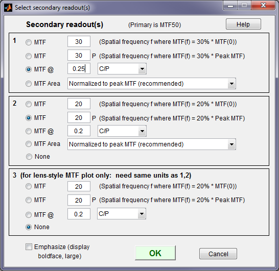
Secondary Readout Clicking opens the window shown on the right. Secondary readout settings are saved between runs. Choices:
Secondary readout controls the secondary readout display in MTF plots. The primary readout is MTF50 (the half-contrast spatial frequency). Three secondary readouts are available with several options. The first defaults to MTF30 (the spatial frequency where MTF is 30%). The third is used only for SFRplus Lens-style MTF plots.
- The upper radio button (MTF) for each readout selects MTFnn, the spatial frequency where MTF is nn% of its low frequency value.
- The second radio button selects MTFnnP, the spatial frequency where MTF is nn% of its peak value: useful with strongly oversharpened edges.
- The third radio button (MTF @ ) selects MTF @ nn units, where nn is a spatial frequency in units of Cycles/pixel, LP/mm, or LP/in. If you select this button, the pixel spacing should be specified in the Cycles per… line in the Plot section of the input dialog box, shown above. A reminder message is displayed if the pixel spacing has been omitted.
- The fourth radio button (MTF Area) selects the area under the MTF curve (below the Nyquist frequency). When it is normalized to the peak MTF it tracks MTF50 for low to moderate sharpening, but, unlike MTF50, it remains constant for oversharpened images. Described in Slanted-Edge MTF measurement consistency.
MTF plot freq selects the maximum display frequency for MTF plots. The default is 2x Nyquist (1 cycle/pixel). This works well for high quality digital cameras, not for imaging systems where the edge is spread over several pixels. In such cases, a lower maximum frequency produces a more readable plot. 1x Nyquist (0.5 cycle/pixel), 0.5x Nyquist (0.25 cycle/pixel), and 0.2x Nyquist (0.1 cycle/pixel) are available.
Edge plot selects the contents of the upper (edge) plot. The edge can be cropped (default) or the entire edge can be displayed. Three displays are available.
- Edge profile (linear) is the edge profile with gamma-encoding removed. The values in this plot are proportional to light intensity. This is the default display.
- Line spread function (LSF) is the derivative of the linear edge profile. MTF is the fast fourier transform (FFT) of the LSF. When LSF is selected, LSF variance (s2), which is proportional to the DxO blur unit, is displayed.
- Edge pixel profile is proportional to the edge profile in pixels, which includes the effects of gamma encoding.
- Edge linear, unnormalized is similar to Edge profile (1.), but not normalized. Useful in diagnosing situations where one channel may be saturating (and affecting MTF measurements).
restores the settings in Options and Settings to their default values.
Settings
Selections in this area affect the calculations as well as the display.
Speedup Checking this box speeds up calculations by skipping noise histogram and SQF calculations. (These plots are unavailable if this box is checked.)
Edge roughness calculation If checked, edge roughness is calculated and results are available for the CSV output file and Edge roughness plot. Slows calculations slightly.
SQF analysis If checked, calculate Acutance/SQF (Subjective Quality Factor). Required for Acutance/SQF plot. Slows calculations slightly.
MTF noise reduction (modified apodization) Reduce noise using the modified apodization technique. Improves MTF accuracy, especially with noisy images, but not an ISO standard calculation. Generally recommended.
Linearization method specifies the method to use for linearizing the slanted edge ROI image data for edge SFR analysis.
Options for SFR analysis include:
-
-
Input gamma value (default) – The inverse of the value entered into the “Gamma (input)” field is used to linearize the data.
-
Note: The input gamma value represents the “forward” (encoding) gamma value (typically around 0.46 = 1/2.2 for sRGB or Adobe RGB color spaces); the inverse (display gamma) is used for linearization. More information on gamma can be found below.
-
-
Gamma calculated from chart contrast – The value selected for the “Chart contrast” setting is used, in combination with the contrast measured from the edge ROI region, to calculate a value for gamma on a per edge ROI basis. The inverse of this gamma is used to linearize the data.
-
The gamma value is estimated from the ratio of the light and dark pixel levels in the slanted-edge region (away from the edge) if the chart contrast ratio (light/dark reflectivity) has been entered (highly recommended to be 10:1 or less for this calculation). Equations for this calculation can be found below.
-
Note: The calculated gamma value(s) are included in the JSON output as the field “gamma_from_chart”, on a per edge ROI basis
-
-
No linearization – The data is not linearized.
-
Note: “Input gamma value” of 1 is equivalent to “No linearization”.
-
-
Gamma is the average slope of log pixel levels as a function of log exposure for light through dark gray tones). It is used to linearize the input data, i.e., to remove the gamma encoding applied by image processing so that MTF can be correctly calculated (using a Fourier transformation, which requires a linear signal). Gamma defaults to 0.5 = 1/2, which is typical of digital camera color spaces, but may be affected by camera or RAW converter settings. Small errors in gamma have little effect on MTF measurements (a 10% error in gamma results in a 2.5% error in MTF50 for a normal contrast target). Gamma should be set to 0.45 or 0.5 when dcraw is used to convert RAW images into sRGB or a gamma=2.2 (Adobe RGB) color space. It is typically around 1 for converted raw images that haven’t had a gamma curve applied. If gamma is set to less than 0.3 or greater than 0.8, the background will be changed to pink to indicate an unusual (possibly erroneous) selection.
A value for gamma can be estimated and used for linearization via the Gamma calculated from chart contrast option (uses the entered chart contrast and the pixel levels from the edge ROI).
A grayscale step chart pattern is included in SFRplus, eSFR ISO and SFRreg Center ([ct]) charts. Gamma is calculated and displayed in the Tonal Response, Gamma/White Bal plot for these modules. Gamma can also be calculated from any grayscale stepchart by running Color/Tone Interactive, Color/Tone Auto, Colorcheck, or Stepchart. [A nominal value of gamma should be entered, even if the value of gamma derived from the chart (described above) is used to calculate MTF.]
| Gamma, Tonal Response, and related concepts contains a detailed explanation of gamma: why it’s used, how to measure it, and much more. |
| Gamma | |
| Gamma is the exponent of the equation that relates image pixel level to luminance. For a monitor or print,
Output luminance = (pixel level)gamma_display When the raw output of the image sensor, which is linear, is converted to image file pixels for a standard color space, the approximate inverse of the above operation is applied. pixel level = (RAW pixel level)gamma_encoding ~= exposuregamma_encoding The total system contrast is gamma_display × gamma_encoding. Standard values of display gamma are 1.8 for older color spaces used in the Macintosh and 2.2 for color spaces used in Windows and the internet, such as sRGB (the default) and Adobe RGB (1998). Gamma from ROI pixel levels— Using the Gamma calculated from chart contrast option along with a value for chart contrast ratio (highly recommended to be ≤ 10 for this calculation), camera gamma can be estimated from the ratio of the light and dark pixel levels P1 and P2 in the slanted-edge region (away from the edge). Starting with \(P_1/P_2 = \text{(chart contrast ratio)}^{gamma\_encoding}\), \(\displaystyle gamma\_encoding = \frac{log(P_1/P_2)}{log(\text{chart contrast ratio})}\) |
|
| The three curves on the right, produced by Stepchart for the Canon EOS-10D, show how Gamma varies with RAW converter settings.In characteristic curves for film and paper, which use logarithmic scales (e.g., density (–log10(absorbed light) vs. log10(exposure)), gamma is the average slope of the transfer curve (excluding the “toe” and “shoulder” regions near the ends of the curve), i.e.,
Gamma is contrast.
See Kodak’s definition in Sensitometric and Image-Structure Data. To obtain the correct MTF, Imatest must linearize the pixel levels— the camera’s gamma encoding must be removed. That is the purpose of Gamma in the SFR input dialog box, which defaults to 0.5, typical for digital cameras. It can, however, vary considerably with camera and RAW converter settings, most notably contrast. Characteristic curves for the Canon EOS-10D with three RAW converter settings are shown on the right. Gamma deviates considerably from 0.5. Gamma = 0.679 could result in a 9% MTF50 error. For best accuracy we recommend measuring gamma using Colorcheck or Stepchart, which provides slightly more detailed results. Confusion factor: Digital cameras rarely apply an exact gamma curve: A “tone reproduction curve” (an “S” curve) is often superposed on the gamma curve to extend dynamic range while maintaining visual contrast. This reduces contrast in highlights and (sometimes) deep shadows while maintaining or boosting it in middle tones. You can see it in curves 1 and 3, on the right. For this reason, “Linear response” (where no S-curves is applied on top of the gamma curve) is recommended for SFR measurements. The transfer function may also be adaptive: camera gamma may be higher for low contrast scenes than for contrasty scenes. This can cause headaches with SFR measurements. But it’s not a bad idea generally; it’s quite similar to the development adjustments (N-1, N, N+1, etc.) in Ansel Adams’ zone system. For this reason it’s not a bad idea to place a Q-13 or Q-14 chart near the slanted edges. To learn more about gamma, read Tonal quality and dynamic range in digital cameras and Monitor calibration. |
3. Canon FVU set to Standard contrast. |
 1.
1. 

Channel is normally left at it’s default value of Y for the luminance channel,
where Y = 0.3*R + 0.59*G + 0.11*B.
In rare instances the R, G, and B color channels might be of interest.
Zone weights Weights of the center, part-way, and corner zones. Used for calculating weighted means of key results, displayed in the Multi-ROI plot. The defaults of 1 (center), 0.75 (part-war), and 0.5 (corners) are for typical pictorial photography; corners should probably be given more weight for technical photography.
Standardized sharpening (not recommended for most applications; may be deprecated in the future) can be selected in a dropdown menu where another setting, Display oversharpening only, is recommended. An image can generally benefit from more sharpening when Undersharpening ((–)Oversharpening, which is closely related to standardized sharpening) is displayed. There may be some sharpening “halo” artifacts in oversharpened images, but moderate amounts of oversharpening is not generally harmful to perceived image quality.
| If Standardized sharpening is selected, standardized sharpening results are displayed as thick red curves and readouts in the edge and MTF plots. If it standardized sharpening results are not displayed, which reduces the visual clutter, results for individual R, G, and B channels are displayed with more prominence (in Imatest Master), and edge roughness is displayed. The MTF .CSV summary file is unaffected.
Standardized sharpening is an algorithm that was developed to allow cameras with different amounts of sharpening to be compared on a reasonable basis. It does so by increasing or decreasing the amount of sharpening to compensate for oversharpened or undersharpened images. Standardized sharpening radius controls the sharpening radius. Its default value of 2 (pixels) is a typical sharpening radius for compact digital cameras, which have tiny pixels. Smaller sharpening radii may be appropriate for digital SLRs, which have larger pixels and tend to have more conservative sharpening. (Imaging-resource.com uses R = 1 for DSLRs.) Sharpening radius varies for different RAW converters and settings. So you may occasionally want to experiment with the sharpening radius. Results with standardized sharpening should not be used for comparing different lenses on the same camera. For more detail, see What is standardized sharpening, and why is it needed for comparing cameras? Standardized sharpening should not be displayed for most applications. If a an edge is too broad for standardized sharpening to work well at the specified radius, the radius is automatically increased unless Fixed sharpening radius in the Settings menu of the Imatest main window has been checked. |
Picture Width and Height defaults to the width and height of the input image in pixels, assuming landscape format, where height < width. note: for using picture height (LW/PH) or (LP/PH) units with cropped images enter the original picture height into the more settings dimensions input.
Line Width per Picture Height (LW/PH) or LP/PH results are correct only if the Picture Height represents the entire uncropped frame. For example, Picture Height should be 2048 for the Canon EOS-10D and 1944 for the Canon G5 (the cameras in the cropped sample files), etc.
Crop location is the position of the center of the selected ROI (Region of interest), expressed as the percentage the distance from the image center to the corner. The orientation of the ROI with respect to the image center is included. It is blank if the input image has not been cropped. Crop location can be entered manually. This is only recommended when that image has been cropped outside of Imatest SFR.
Additional parameters (all optional) for Excel .CSV output
contains a detailed description of the camera, lens, and test conditions. EXIF data is entered, if available, but can be overridden by manual settings. Description & settings is particularly useful for annotating the test system (it is displayed in MTF Compare).These settings are optional but can be useful when several tests are run for different lenses, focal lengths, apertures, or other settings. The settings are displayed next to the MTF plots. They are saved and reused in subsequent runs for files with the same pixel dimensions. If EXIF data is available (currently, only in JPEG files) it overrides the saved settings. The button clears all entries.
ISO standard SFR If this checkbox is checked, SFR calculations are performed according to the ISO 12233 standard, and the y-axis is labeled SFR (MTF) (ISO standard). This method is slightly less accurate than the normal Imatest calculation, which incorporates a number of refinements, including a better edge detection algorithm and a second-order polynomial fit to the average edge for a more accurate estimate of SFR in the presence of lens distortion. This box is normally left unchecked; it should only be used for comparing normal Imatest calculations to the ISO standard. The difference is typically very small.
When entries are complete, click . A Calculating…
box appears to let you know that calculations are proceeding. Results appear in individual windows called Figures (Matlab’s standard method of displaying plots). Figures can be examined, resized, maximized, and closed at will. A zoom function is also available. Their contents are described in the pages on Imatest SFR results: MTF (Sharpness) plot, Chromatic Aberration, Noise, and Shannon Capacity plot, and Multiple ROI (Region of Interest) plot.
Warnings
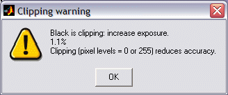
| A Clipping warning is issued if more than 0.5% of the pixels are clipped (saturated), i.e., if dark pixels reach level 0 or light pixels reach the maximum level (255 for bit depth = 8). This warning is emphasized if more than 5% of the pixels are clipped. Clipping reduces the accuracy of SFR results. It makes measured sharpness better than reality. |
 |
|
|
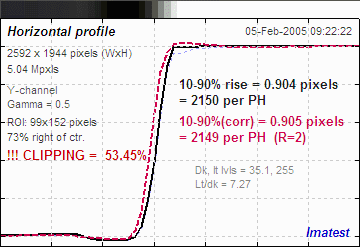
The percentage of clipped pixels is not a reliable index of the severity of clipping or of the measurement error. For example, it is possible to just barely clip a large portion of the image with little loss of accuracy. The plot on the right illustrates relatively severe clipping, indicated by the sharp “shoulder” on the black line (the edge without standardized sharpening). The sharp corner makes the MTF look better than reality. The absence of a sharp corner may indicate that there is little MTF error. Clipping can usually be avoided with a correct exposure– neither too dark nor light. A low contrast target is recommended for reducing the likelihood of clipping: it increases exposure latitude and reduces the sensitivity of the MTF results to errors in estimating gamma. |
 Clipping warnings Clipping warnings |
| Too many open FiguresFigures can proliferate if you do a number of runs, especially SFR runs with multiple regions, and system performance suffers if too many Figures are open. You will need to manage them. Figures can be closed individually by clicking X on the upper right of the Figure or by any of the usual Windows techniques. You can close them all by clicking Close figures in the Imatest main window. For large batch runs, the Close figures after save checkbox in the SFR Save dialog box prevents a buildup of open figures. | Clicking on Figures during calculations can confuse Matlab. Plots can appear on the wrong figure (usually distorted) or disappear altogether. Wait until all calculations are complete— until the Save or Imatest main window appears— before clicking on any Figures. |
Saving the results
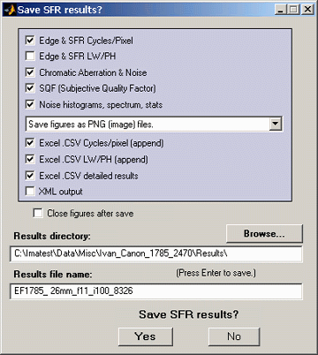
SFR save dialog box
At the completion of the SFR calculations the Save SFR results? dialog box appears, except in Express mode, which uses previous settings. It allows you to choose which results to save and where to save them. The default is subfolder Results of the data file folder. You can change to another existing folder, but new results directories must first be created outside of Imatest using a utility such as Windows Explorer. (This is a limitation of this version of Matlab.)
Figures can be saved as either PNG files (a standard losslessly-compressed image file format) or as Matlab FIG files, which can be opened by the button in the Imatest main window. Fig files can be manipulated (zoomed and rotated), but they tend to require more storage than PNG files.
Saved figures, CSV, and XML files are given names that consist of a root file name (which defaults to the image file name) with a suffix added. Examples:
Canon_17-40_24_f8_C1_1409_YR7_cpp.png
Canon_17-40_24_f8_C1_1409_YR7_MTF.csv
The root file name, Canon_17-40_24_f8_C1_1409_YR7, can be overridden by entering another name in the Results root file name: box. Be sure to press the Enter key. This feature does not work with batch runs.
Checking Close figures after save is recommended for preventing a buildup of figures (which slows down most systems) in batch runs.
When multiple ROIs are selected, the Save results? dialog box appears only after the first set of calculations. The remaining calculations use the same Save settings. Save results? is omitted entirely in an Express run for repeated images.
The first four checkboxes are for the figures, which can be examined before the boxes are checked or unchecked. After you click on Yes or No, the selections are saved, then the Imatest main window reappears.
Result file names— The roots of the file names are the same as the image file name. The channel (Y, R, G, or B) is included in the file name. If a Region of Interest has been selected from a complete digital camera image, information about the location of the ROI is included in the file name following the channel. For example, if the center of the ROI is above-right of the image, 20% of the distance from the center to the corner, the characters AR20 are included in the file name.
(default location: subdfolder Results)
| Figures (.PNG image files) | |
| filename_YA17_cpp.png | Plot with x-axis in cycles/pixel (c/p), Y-channel,17% of the way to the corner above the center of the uncropped image. |
| filename_YA17_lwph.png | Plot with x-axis in Line Widths per Picture Height (LW/PH). |
| filename_YA17_ca.png | Plot of Chromatic Aberration, with noise statistics and Shannon information capacity. |
| Excel .CSV (ASCII text files that can be opened in Excel) | |
| CSV output files are explained in detail below. Click link for detail on individual file. | |
| SFR_cypx.csv | (Database file for appending results: name does not change). Displays 10-90% rise in pixels and MTF in cycles/pixel (C/P). |
| SFR_LWPH.csv | (Database file for appending results: name does not change). Displays 10-90% rise in number/Picture Height (/PH) and MTF in Line Widths per Picture Height (LW/PH). |
| filename_YA17_MTF.csv | Excel .CSV file of MTF results for this run. All channels (R, G, B, and Y (luminance) ) are displayed.The first row has the headers: cy/pxl, LW/PH, MTF(nchan), MTF(corr), MTF(R), MTF(G), MTF(B), MTF(Y), where nchan is the selected channel and corr is the selected channel with Standardized sharpening applied. The remaining lines contain the data. Can easily be plotted or combined with data from other files. |
| filename_Y_multi.csv | Excel .CSV file of summary results for a multiple ROI run. |
| filename_Y_sfrbatch.csv | Excel .CSF file combining the results of batch runs (several files) with multiple ROIs. Particularly useful for generating easily-readable Excel plots. |
The PNG files are identical to the Imatest Figures, except that the background is white instead of gray.
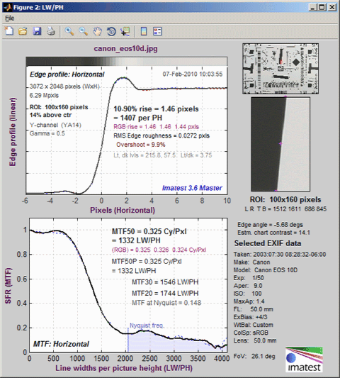 Average edge and MTF plot (primary results of SFR)
MTF is explained in Sharpness: What is it and how is it measured? MTF curves and Image appearance contains several examples illustrating the correlation between MTF curves and perceived sharpness.
Repeated runs
 ROI Repeat dialog box. Automatic ROI refine is not in Studio.
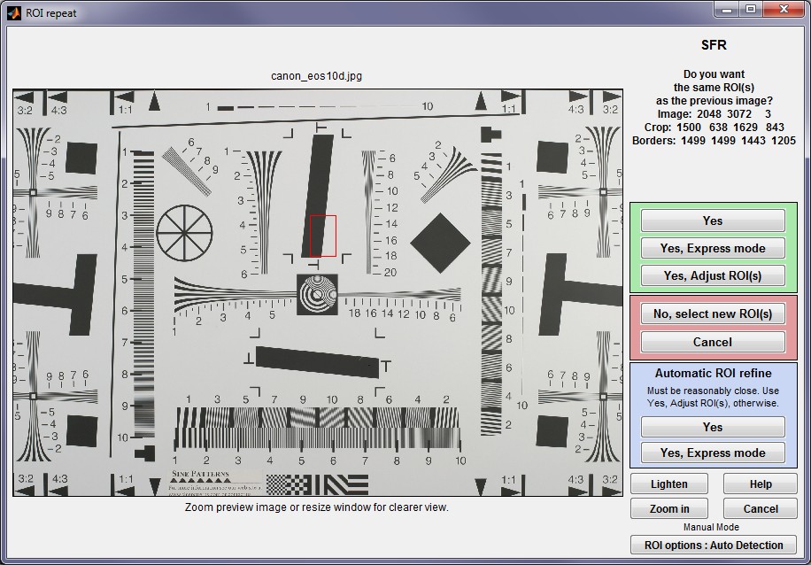
If SFR was recently run with an image of the same pixel dimensions, the ROI Repeat dialog box opens and asks, “Do you want the same ROIs as the previous image?“
| Yes | Use the previous crop. Open SFR input dialog box. |
| Yes, Express mode | Use previous crop and run in Express mode, i.e., do not open the input dialog box; use saved data instead. Save dialog boxes are also omitted. Some warnings are suppressed. Speeds up repeated runs, e.g., testing several apertures. |
| Yes, Adjust ROI | Open a fine adjustment dialog box (shown below), starting with the previous selection.Useful for a sequence of runs with similar, but not identical, framing.Imatest Studio: Only available when a single ROI is selected.Imatest Master : For multiple ROIs, a window that allows ROIs to be shifted and changed in magnification is opened. |
| No | Crop the image using the Select the ROI… dialog box described above. |
| Cancel | Cancel the run. Return to the main Imatest window. |
| Automatically refine ROIsYes | Imatest Master only Refine previous crop (see description below) and run in Express mode. |
| Automatically refine ROIsYes, Express mode | Imatest Master only Refine previous crop (see description below). Open SFR input dialog box. |
The meaning of the answers is self-evident except for “Yes, Express mode.“This button is the same as “Yes,” except that the Input dialog box and the two Save dialog boxes (for individual Figures and for the multiple ROI figures at the end) are omitted. Default settings or settings saved from previous runs are used. The clipping warning boxes are suppressed. This speeds up repeated runs; for example, it’s very handy when you are testing a lens at several apertures (f/2.8, f/4, f/5.6, etc.).
Automatic ROI refinement (Imatest Master only)
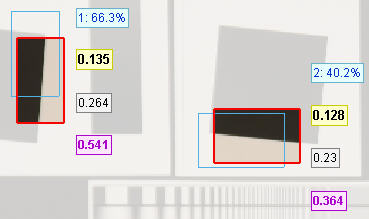
Results of automatic ROI Refinement:
Original (cyan) and refined (bold red)
This option is very useful for sequences of runs where chart alignment varies slightly; it can be especially valuable for Imatest API in manufacturing environments.
The Imatest Master ROI repeat dialog box offers two options in the light blue box on the right (Yes and Yes, Express mode) that include automatic ROI refinement. Results of the refinement are shown in the crop of the Multi-ROI 2D summary plot on the right. The original (incorrect) ROIs are shown as cyan rectangles; the automatically refined (shifted) ROIs are shown as bold red rectangles filled with the full contrast image.
Automatic ROI refinement works best with charts dedicated to SFR measurement such as the SFR SVG test charts. It may not work as well with the ISO 12233 charts because of the narrowness of the SFR strips and the presence of interfering patterns.
The length of the ROIs should be no larger than 85% of the length of the edge to be measured. Automatic refinement will succeed if no more than 30% of the ROI length is off the edge. The modified ROI is not saved in imatest.ini.
Storing and recovering multiple ROI regions
Multiple ROI regions (the result of the initial entry or fine adjustment, but not automatic refinement) are stored in imatest.ini, which can be opened for editing by pressing Settings, View settings (ini file) from the Imatest main window . The number of regions, image width and height, and regions are stored under [SFR] and have the following appearance.
nroi = 9
nwid_save = 3888
nht_save = 2592
roi_mult = 3347 2356 3555 2697;1813 1032 2031 1412;1813 3789 2040 4163;5159 …
Each group of four values ( x1 y1 x2 y2 ) delimited by semicolons (;) represents one ROI. The regions are separated by tabs, but spaces work equally well. The origin (x = y = 0) is at the upper-right of the image (i.e., y increases going down).
Multiple ROI regions are stored in identical format ( roi_mult = 3342 2356 3550 2697 ; … ) in the multi-ROI CSV output file, which has a name of the form input_file_Y_multi.csv. To reuse an old set of ROIs, copy the four lines from the CSV file, paste them into imatest.ini replacing the previous entries, then save (ctrl-S).
Excel .CSV (Comma-Separated Variables) and XML output
Imatest SFR creates or updates output files for use with Microsoft Excel. The files are in CSV (Comma-Separated Variable) format, and are written to the Results subfolder by default. .CSV files are ASCII text files that look pretty ugly when viewed in a text editor:
| File ,Date/time ,PH,Ch,H/V,10-90U,10-90C,Over-,Over-,MTF50U,MTF50C,MTF,Camera,Lens,FL,f-stop,Loc,Misc.,,,,,/PH,/PH,shoot%,sharp%,LW/PH,LW/PH,Nyq,,,(mm),,,settings canon_eos10d_sfr.jpg,2004-03-19 22:21:34, 2048,Y,H, 1422, 1447, 19.5, -0.7, 1334, 1340,0.154,,,,, canon_g5_sfr.jpg,2004-03-19 22:24:30, 1955,Y,H, 1973, 1301, 48.0, 21.3, 1488, 1359,0.268,Canon G5,—,14,5.6,ctr, sigma_sd9_sfr.jpg,2004-03-19 22:27:55, 1504,Y,H, 1432, 1676, 2.4, -7.7, 1479, 1479,0.494,,,,, sigma_sd10_sfr.jpg,2004-03-19 22:28:32, 1504,Y,H, 1563, 1628, 11.9, -2.0, 1586, 1587,0.554,,,,, |
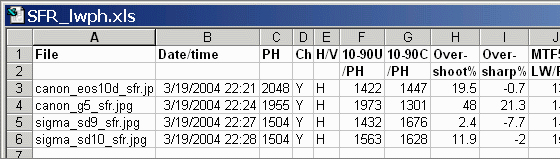
But they look fine when opened in Excel.
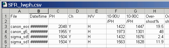
.CSV files can be edited with standard text editors, but it makes more sense to edit them in Excel, where columns as well as rows can be selected, moved, and/or deleted. Some fields are truncated in the above display, and Date/time is displayed as a sequence of pound signs (#####…).
The format can be changed by dragging the boundaries between cells on the header row (A, B, C, …) and by selecting the first two rows and setting the text to Bold. This makes the output look better. The modified file can be saved with formatting as an Excel Worksheet (XLS) file. This, of course, is just the beginning.
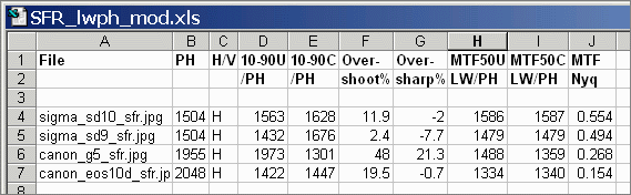
It’s easy to customize the Excel spreadsheet to your liking. For example, suppose you want to make a concise chart. You can delete Date/time (Row B; useful when you’re testing but not so interesting later) and Channel (all Y = luminance). You can add a blank line under the title, then you can select the data (rows A4 through J7 in the image below) and sort on any value you choose. Corrected MTF50 (column I) has been sorted in descending order. Modified worksheets should be saved in XLS format, which maintains formatting.
There are no limits. With moderate skill you can plot columns of results. I’ve said enough. ( I’m not an Excel expert! )
Database files
Two .CSV files are used as a database for storing data from SFR runs. If possible, data from the current run is appended to these files. A third file for storing MTF and other summary data is described below.
- SFR_cypx.csv displays 10-90% rise in pixels and MTF in cycles/pixel (C/P).
- SFR_lwph.csv displays 10-90% rise in number/Picture Height (/PH) and MTF in Line Widths per Picture Height (LW/PH).
When SFR is run, it looks for the two files in the same folder as the slanted-edge input image. If it doesn’t find them, it creates them, writes the header lines, then writes a line of data for the run. If it finds them, it appends data for the run to the files. You can rapidly build a spreadsheet by doing repeated runs from files in the same folder. The following table contains
the entries. Camera and the entries that follow are all optional. With the exception of Loc, which is calculated when the ROI is manually selected, they are only added if you answer y
to the question, Additional data for Excel file?, and enter them manually.
| File | File name. Should be concise and descriptive. |
| Date/time | Date and time in sortable format. Displays differently in Excel. |
| PH | Picture Height (in SFR_lwph.csv only). |
| Ch | Channel. Y (luminance) [default], R, G, or B. |
| H/V | Horizontal or Vertical measurements. (A vertical chart gives you horizontal rise and MTF, etc.) |
| 10-90U | 10-90% rise distance, uncorrected. |
| 10-90C | 10-90% rise distance, corrected with standard sharpening. |
| Overshoot% | Overshoot of the edge. |
| Oversharp% | Oversharpening: the amount of sharpening relative to the standard sharpening.If negative, the image is undersharpened. |
| MTF50U | MTF50 (frequency where MTF = 50%), uncorrected. |
| MTF50C | MTF50 (frequency where MTF = 50%), corrected with standard sharpening. |
| MTF Nyq | MTF at Nyquist frequency. May indicate the likelihood of aliasing problems. But it not an unambiguous indicator because aliasing is related to sensor response, and MTF at Nyquist is the product of sensor response, the demosaicing algorithm, and sharpening, which can boost response at Nyquist for radii less than 1. |
| Camera | Camera name. This entry and those that follow are manually-entered and optional. |
| Lens | Lens name. Only for DSLRs with interchangeable lenses. |
| FL (mm) | Focal length in mm. |
| f-stop | Aperture |
| Loc | Location of image (center, edge, corner, etc.) |
| Misc. settings | Anything else: RAW converter, Sharpening setting, etc. |
| Secondary readout(s) |
If secondary readouts (up to two) are present, they are appended to the end of the line as name,value pairs. Example: ,MTF20,0.26817,MTF @ 0.25 C/P,0.22835 |
Tips
- To build a spreadsheet of results, put the slanted-edge image files in the same folder. File names should be concise and descriptive. If you’ve run SFR from image files in different folders, there will be multiple versions of the CSV files. They can be easily combined with a text editor on in Excel.
- Neither SFR_cypx.csv nor SFR_lwph.csv should be open in Excel when you run SFR. If either is open, an error message will appear instructing you to close them.
Summary .CSV and XML files for MTF and other data
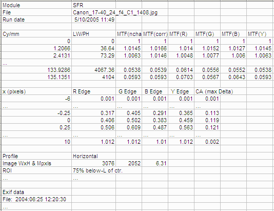
An optional .CSV (comma-separated variable) output file contains results for MTF and other data. Its name is [root name]_[channel location]_MTF.csv, where channel is (R, G, B, or Y) and the location BL75 means below-left, 75% of the distance to the corner (from the center). An example is Canon_17-40_24_f4_C1_1408_YBL75_MTF.csv. Excerpts are shown below, opened in Excel.
A portion of the summary CSV file, opened in Excel
The format is as follows:
| Line 1 | Imatest, release (1.n.x), version (Light, Pro, Eval), module (SFR, SFR multi-ROI, Colorcheck, Stepchart, etc.). |
| File | File name (title). |
| Run date | mm/dd/yyyy hh:mm of run. |
| (blank line) | |
| Tables | Separated by blank lines if more than one. Two tables are produced. |
| The first table contains MTF. The columns are Spatial frequency in Cy/mm, LW/PH, MTF (selected channel), MTF (Red), MTF (Green), MTF (Blue), MTF (Luminance = Y). (…) represent rows omitted for brevity. | |
| The second table contains the edge. Columns are x (location in pixels), Red edge, Green edge, Blue edge, Luminance (Y) edge, and Chromatic Aberration (the difference between the maximum and minimum). | |
| (blank line) | |
| Additional data | The first entry is the name of the data; the second (and additional) entries contain the value. Names are generally self-explanatory (similar to the figures). |
| (blank line) | |
| EXIF data | Displayed if available. EXIF data is image file metadata that contains important camera, lens, and exposure settings. By default, Imatest uses a small program, jhead.exe, which works only with JPEG files, to read EXIF data. To read detailed EXIF data from all image file formats, we recommend downloading, installing, and selecting Phil Harvey’s ExifTool, as described here. |
This format is similar for all modules. Data is largely self-explanatory. Enhancements to .CSV files will be listed in the Change Log.
The optional XML output file contains results similar to the .CSV file. Its contents are largely self-explanatory. It is stored in [root name].xml. XML output will be used for extensions to Imatest, such as databases, to be written by Imatest and third parties. Contact us if you have questions or suggestions.
An optional .CSV file is also produced for multiple ROI runs. Its name is [root name]_multi.csv.
