Introduction – Examples – Oversharpening and Undersharpening
Examples – Unsharp masking (USM) – Links
Introduction to sharpening
Sharpening is an important part of digital image processing. It restores some of the sharpness lost in the lens and image sensor. Every digital image intended for human viewing benefits from sharpening at some point in its workflow— in the camera, the RAW conversion software, and/or the image editor. Sharpening has a bad name with some photographers because it has been overdone in some cameras (mostly low-end compacts and camera phones), resulting in ugly “halo” effects near edges. But it’s entirely beneficial when done properly.
The JPEG image output of almost every digital camera is sharpened to some degree. Some models sharpen images far more than others— often excessively for large prints. This makes it difficult to compare cameras and determine their intrinsic quality unless RAW images are available. [Imatest’s standardized sharpening approach has long been deprecated, but the new image information metrics provide a basis for an approximate comparison.] The Imatest Image Processing module lets you choose one of two sharpening functions: simple (standard) sharpening— a 2D version of the 1D example below, which is common in cameras, or USM sharpening, which is rare in cameras (because it is more computation-intensive), but is standard in off-camera raw conversion and editing software.
The sharpening process
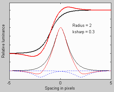
Sharpening on a line and edge
A simple sharpening algorithm subtracts a fraction of neighboring pixels from each pixel, as illustrated on the right. The thin black curve in the lower part of the image is the input to the sharpening function: it is the camera’s response to a point or a sharp line (called the point or line spread function). The two thin dashed blue curves are replicas of the input, reduced in amplitude (multiplied by –ksharp ⁄ 2) and shifted by distances of ±2 pixels (typical of the sharpening applied to compact digital cameras). This distance is called the sharpening radius RS. The thin red curve the impulse response after sharpening— the sum of the black curve and the two blue curves. The thick black and red curves (shown above the thin curves) are the corresponding edge responses, unsharpened and sharpened.
Sharpening increases image contrast at boundaries by reducing the rise distance. It can cause an edge overshoot. (The upper red curve has a small ovrshoot.) Small overshoots enhance the perception of sharpness, but large overshoots cause “halos” near boundaries that may look good in small displays such as camera phones, but can become glaringly obvious at high magnifications, detracting from image quality.
Sharpening also boosts MTF50 and MTF50P (the frequencies where MTF drops to 50% of its low frequency and peak values, respectively), which are indicators of perceived sharpness. (MTF50P is often preferred because it’s less sensitive to strong sharpening.) Sharpening also boosts noise, which is can be a problem with noisy systems (small pixels or high ISO speeds).
|
Sharpening is a linear process that has a transfer function.The formula for the simple sharpening algorithm illustrated above is, \(\displaystyle L_{sharp} (x) = \frac{L(x)\: -\: 0.5k_{sharp} (L(x-V) + L(x+V))}{1-k_{sharp}}\) L(x) is the input pixel level and Lsharp(x) is the sharpened pixel level. ksharp is the sharpening constant (related to the slider setting scanning or editing program). V is the shift used for sharpening. \(V =R_S / d_{scan}\) where R is the sharpening radius (the number of pixels between original image and shifted replicas) in pixels. dscan is the scan rate in pixels per distance. 1/dscan is the spacing between pixels. The sharpening algorithm has its own MTF (the Fourier transform of Lsharp(x) ⁄ L(x)). \(\displaystyle MTF_{sharp}(f) = \frac{1-k_{sharp}\cos(2\pi f V)}{1-k_{sharp}}\) This equation boosts response at high spatial frequencies with a maximum where \(\cos(2\pi f V) = \cos (\pi) = -1\) or \( f = \frac{1}{2V} = \frac{d_{scan}}{2R_S}\). This is equal to the Nyquist frequency, \( f_{Nyq} = d_{scan}/2\), for RS = 1 and lower for RS > 1. Actual image sharpening is a two dimensional operation. |
Sharpening examples
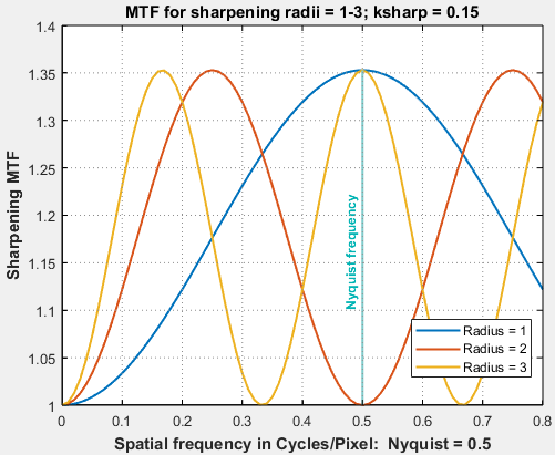
Sharpening transfer function for radii RS = 1, 2, and 3 pixels (Note that the y-axis is 1 at the bottom.)
The plot on right shows the transfer function (MTF) for sharpening with strength ksharp = 0.15 and sharpening radius RS = 1, 2, and 3. Note the the bottom of the plot is MTF = 1 (not 0).
At the widely-used sharpening radius of 2, the transfer function reaches its maximum value at half the Nyquist frequency (f = fNyq/2 = 0.25 cycles/pixel), drops back to 1 at the Nyquist frequency (fNyq = 0.5 C/P), then bounces back to the maximum at 1.5×fNyq = 0.75 C/P.
Note that the sharpening transfer function is cyclic, i.e., it oscillates. This can have serious consequences for some MTF measurements on sharpened images.
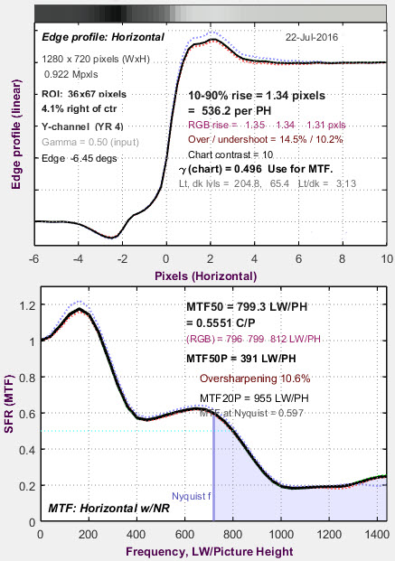
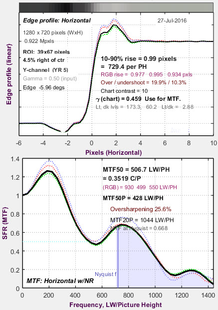
The MTF plots below are for two images sharpened with radius ≅ 3. This camera is quite sharp prior to sharpening— there is significant energy above the Nyquist frequency. There is a response dip response around MTF ≅ 400-500 LW/PH that causes MTF50 (the spatial frequency where MTF is 50% of the low frequency value) to become ext–remely unstable—799 and 507 LW/PH for the similar images. This is a fairly rare (extreme) case, but it’s something to watch for. MTFnn at lower levels— MTF20, MTF10, etc.— can be even more unstable.
This camera would have performed better with RS ≤ 2.
 |
 |
| Be cautious about using strong sharpening with large sharpening radii (RS > 3). Cyclic response can lead to unexpected bumps in the MTF response curve that can severely distort summary metrics such as MTF50, MTF20, etc. Large sharpening radii have characteristic signatures— thick “halos” and low frequency peaks in the MTF response. We recommend keeping RS ≤ 2 unless there is a compelling reason to make it larger. |
A camera’s sharpening can be analyzed if you have access to raw (unprocessed) and JPEG (standard processed camera output) files using the Imatest MTF Compare module.
|
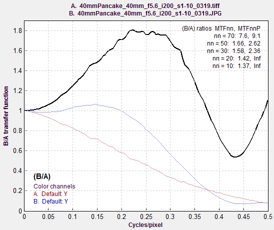
Here is an example from the Canon EOS-6D full-frame DSLR. A JPEG image (blue curve) with sharpening slightly reduced is compared with a TIFF image converted from raw by dcraw (with no sharpening and noise reductions). The exact same exposure and regions were used for each curve (both JPG and raw files were saved).The peak at 0.25 cycles/pixel indicates that sharpening with radius = 2 was used. The plot deviates from the ideal plot (for a very simple sharpening algorithm) for spatial frequencies above 0.35 C/P. The EOS-6D allows you to change the amount of sharpening but not the radius for camera JPEGs. (I’m not happy with this limitation.) Sharpening MTF, comparing the same image, |
 |
 |
 |
|
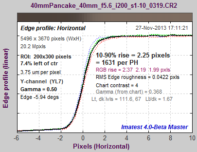
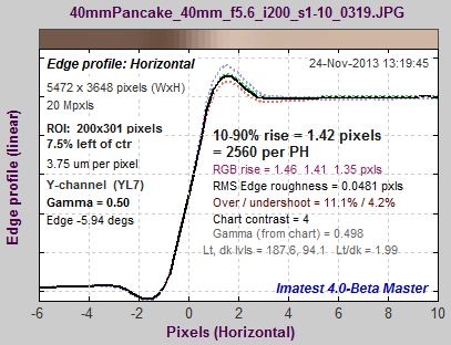
Corresponding edges for the Canon EOS-6D: unsharpened (left), sharpened (right) These curves (and the curves below for the Panasonic Lumix LX7) show how MTF curves (in the MTF Compare plots) correlate to edge response. The modest amount of overshoot (“halo”) on this edge would not be objectionable at any viewing magnification. Better overall performance would be achieved with a sharpening radius of RS = 1 and an appropriate sharpening amount. |
|
|
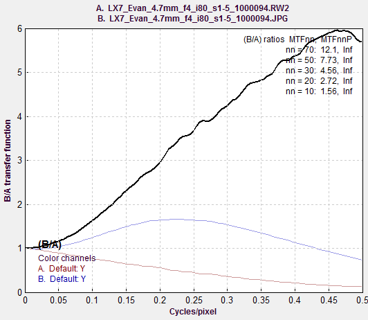
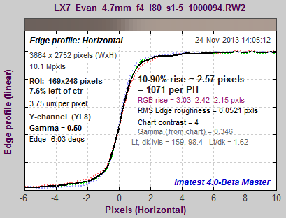
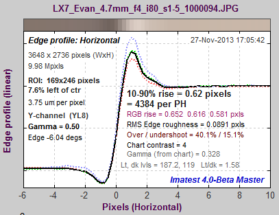
Here is another example from the Panasonic Lumix LX7. As with the Canon, the same exposure and regions are used: one from a JPEG image (default sharpening, which is very strong), and one from a raw image, converted with no sharpening or noise reduction.The sharpening radius of 1 makes for a sharper image at the pixel level than JPEGs straight out of the EOS-6D, above. Of course the EOS-6D has twice as many pixels (20 vs. 10), but the difference in sharpening accounts for the relatively close sharpness noted in the post, Sharpness and Texture from Imaging-Resource.com. Sharpening MTF, comparing the same image, |
 |
 |
 |
|
Corresponding edges for the Panasonic Lumix LX7: unsharpened (left), sharpened (right) These curves show how MTF curves (red for raw and blue for JPEG (sharpened) in the MTF Compare plot, above) correlate to edge response. The LX7 is much more strongly sharpened in both frequency and spatial domains than the EOS-6D (above). It also has a smaller sharpening radius (RS = 1). The strong sharpening would be visible and objectionable at large magnifications, though is results in some impressive measurements: sharpened MTF50P is 2600 LW/PH vs. 2239 for the EOS-6D, which has twice as many pixels. (The EOS-6D would do better,both visually and numerically (i.e., better measurements) with a sharpening radius of RS = 1 instead of 2.) |
|
Oversharpening and Undersharpening
Oversharpening or undersharpening is the degree to which an image is sharpened relative to the standard sharpening value. If it is strongly oversharpened (oversharpening >about 30%), “halos” might be visible near edges of highly enlarged images. The human eye can tolerate considerable oversharpening because displays and the eye itself tend to blur (lowpass filter) the image. (Machine vision systems are not tolerant of oversharpening.) There are cases where highly enlarged, oversharpened images might look better with less sharpening. If an image is undersharpened (oversharpening < 0; “undersharpening” displayed) the image will look better with more sharpening. Basic definitions:
Oversharpening = 100% (MTF( feql ) – 1)
where feql = 0.15 cycles/pixel = 0.3 * Nyquist frequency for reasonably sharp edges (MTF50 ≥ 0.2 C/P).
feql = 0.6*MTF50 for MTF50 < 0.2 C/P (relatively blurred edges)
When oversharpening < 1 (when MTF is lower at feql than at f = 0), the image is undersharpened, and
Undersharpening = –Oversharpening is displayed.
If the image is undersharpened (the case for the EOS-1Ds shown below), sharpening is applied to the original response to obtain Standardized sharpening; if it is positive (if MTF is higher at feql than at f = 0), de-sharpening is applied. (We use “de-sharpening” instead of “blurring” because the inverse of sharpening is, which applied here, is slightly different from conventional blurring.) Note that these numbers are not related to the actual sharpening applied by the camera and software.
Examples: under and oversharpened images
 Undersharpened image Undersharpened image |
 Oversharpened image |
|
The 11 megapixel Canon EOS-1Ds DSLR is unusual in that it has very little built-in sharpening (at least in this particular sample). The average edge (with no overshoot) is shown on top; the MTF response is shown on bottom. The black curves are the original, uncorrected data; the dashed red curves have standardized sharpening applied. Standardized sharpening results in a small overshoot in the spatial domain edge response, about what would be expected in a properly (rather conservatively) sharpened image. It is relatively consistent for all cameras. |
The image above is for the 5 megapixel Canon G5, which strongly oversharpens the image— typical for a compact digital camera.A key measurement of rendered detail is the inverse of the 10-90% edge rise distance, which has units of (rises) per PH (Picture Height). The uncorrected value for the G5 is considerably better than the 11 megapixel EOS-1Ds (1929 vs. 1505 rises per PH), but the corrected value (with standardized sharpening) is 0.73x that of the EOS-1Ds. Based on vertical pixels alone, the expected percentage ratio would be 100% (1944/2704) = 0.72x. MTF50P is not shown. It is displayed when Standardized sharpening is turned off; it can also be selected as a Secondary readout. For this camera MTF50P is 0.346 cycles/pixel or 1344 LW/PH, 9% lower than MTF50. It is a better sharpness indicator for strongly oversharpened cameras, especially for cameras where the image will not be altered in post-processing. |
|
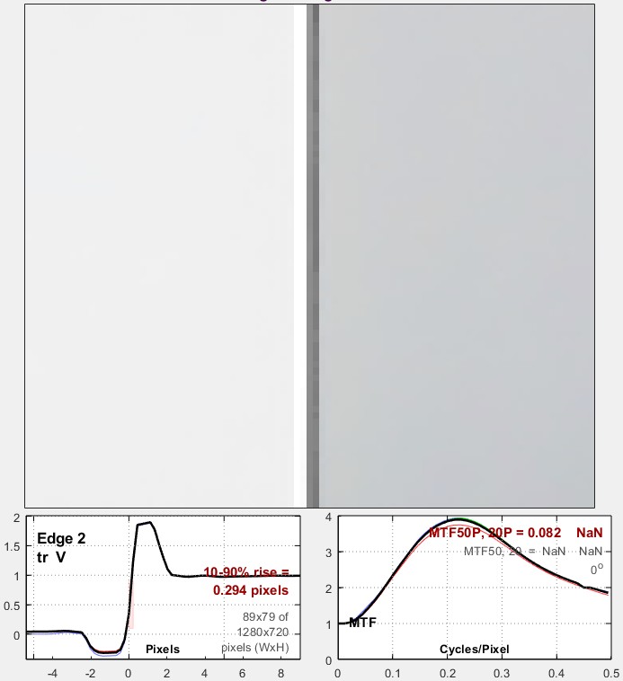
Here is an example of an insanely oversharpened image, displayed in Rescharts with Show edge crop & MTF checked. This displays small edge and MTF plots under a large image of the slanted-edge region. When customers send us problem images we do our best to educate them about how it can be improved. Everything is wrong about this image. To begin with it’s perfectly vertical, not slanted as we recommend (a slant of ≥ 2 degrees is usually sufficient). This means the result will be overly sensitive to sampling (subpixel positioning) and won’t be consistent from image to image. It’s also extremely oversharpened, and both the negative and positive peaks are strongly clipped (flattened), which makes it difficult to determine the severity of the oversharpening. Clipping invalidates the assumption of linearity used for MTF calculations, and makes the result completely meaningless— MTF curves can be much more extended than reasonable. In this case, MTF never drops below 1 at high frequencies, so MTF50 and MTF20 are not even defined. |
 |
These results illustrate how uncorrected rise distance and MTF50 can be misleading when comparing cameras with different pixel sizes and degrees of sharpening. MTF50P is slightly better for comparing cameras when strong sharpening is involved.
Uncorrected MTF50 or MTF50P are, however, appropriate for designing imaging systems or comparing lens performance (different focal lengths, apertures, etc.) on a single camera.
Unsharp Masking (USM)
“Unsharp masking” (USM) and “sharpening” are often used interchangeably, even though their mathematical algorithms are different. The confusion is understandable but rarely serious because the end results are visually similar. But when sharpening is analyzed in the frequency domain the differences become significant.
“Unsharp masking” derives from the old days of film when a mask for a slide, i.e., positive transparency, was created by exposing the image on negative film slightly out of focus. (Here is a great example from a PBS broadcast. (Alternate Youtube page.)) The next generation of slide or print was made from a sandwich of the original transparency and the fuzzy mask. This mask served two purposes.
- It reduced the overall image contrast of the image, which was often necessary to get a good print.
- It sharpened the image by increasing contrast near edges relative to contrast at a distance from edges.
Unsharp masking was an exacting and tedious procedure which required precise processing and registration. But now USM can be accomplished easily in most image editors, where it’s used for sharpening. You can observe the effects of USM (using the Matlab imsharpen routine) in the Imatest Image Processing module, where you can adjust the blur radius, amount, and threshold settings.
Most cameras perform regular sharpening rather than USM because it’s faster— USM requires a lot more processing power.
Thanks to the central limit theorem, blur can be approximated by the Gaussian function (Bell curve).
$$\displaystyle \text{Blur} = \frac{e^{-x^2 / 2\sigma_x^2}}{\sqrt{2\pi \sigma_x^2}}$$
σx corresponds to the sharpening radius, R. The unsharp masked image can be expressed as the original image summed with a constant times the convolution of the original image and the blur function, where convolution is denoted by *.
$$\displaystyle L_{USM}(x) = L(x) – k_{USM} \times \text{Blur} = L(x) \times \frac{\delta(x) – k_{USM} e^{-x^2/2\sigma_x^2} / \sqrt{2\pi \sigma_x^2}}{1 – k_{USM} / \sqrt{2\pi}}$$
L(x) is the input pixel level and LUSM(x) is the USM-sharpened pixel level. kUSM is the USM sharpening constant (related to the slider setting scanning or editing program). L(x) = L(x) * δ(x), where δ(x) is a delta function.
The USM algorithm has its own MTF. Using
$$ F(e^{-px^2}) = \frac{e^{-a^2/4p}}{\sqrt{2p}}, $$ where F is the Fourier transform,
$$MTF_{USM} (f) = \frac{1 – k_{USM} e^{-f^2 \sigma_x^2 /2} / \sqrt{2\pi}}{1 – k_{USM} / \sqrt{2 \pi}} = \frac{ 1 – k_{USM} e^{-f^2 / 2 f_{USM}^2} / \sqrt{2\pi}}{1 – k_{USM}/ \sqrt{2\pi}}$$
where fUSM = 1/σx. This equation boosts response at high spatial frequencies, but unlike sharpening, response doesn’t reach a peak then drop— it’s not cyclic. Actual sharpening is a two dimensional operation.
Links
How to Read MTF Curves by H. H. Nasse of Carl Zeiss. Excellent, thorough introduction. 33 pages long; requires patience. Has a lot of detail on the MTF curves similar to the Lens-style MTF curve in SFRplus. Here is an interesting list of Zeiss technical articles.
Understanding MTF from Luminous Landscape.com has a much shorter introduction.
Understanding image sharpness and MTF A multi-part series by the author of Imatest, mostly written prior to Imatest’s founding. Moderately technical.
Bob Atkins has an excellent introduction to MTF and SQF. SQF (subjective quality factor) is a measure of perceived print sharpness that incorporates the contrast sensitivity function (CSF) of the human eye. It will be added to Imatest Master in late October 2006.
Optikos makes instruments for measuring lens MTF. Their 64 page PDF document, How to Measure MTF and other Properties of Lenses, is of particular interest.