|
Image Processing has been superseded by Simatest, which does much more — it allows complete camera systems to be simulated. Here are the key links. [We do not plan to deprecate Image Processing.] Simatest: Overview – Compact introduction to Simatest. Recommended for getting started. Simatest ISP/Camera Simulator — Instructions and Reference – Very detailed Simatest examples – Examples of how Simatest can be used. Compares simulations to measurement. Much more readable than this long page. Image Sensor Noise – measurement and modeling – using raw files for image sensor Dynamic Range and Simatest |
Operation – Image processing blocks – Standard sharpening – Displays and analysis – Remosaicing
Optical Character Recognition (OCR) – Face and People Detection
The Imatest Image Processing module simulates a number of image processing operations, including
- image degradations such as noise, fog, and blur, as well as
- image enhancements such as applying a Color Correction Matrix, tone mapping (used in High Dynamic Range (HDR) imaging), Sharpening (standard and Unsharp Mask (USM)), and bilateral filtering.
You can instantly observe the visible effects of these operations by switching between unprocessed and processed images, and you can see how processing affects several measurements, including SSIM, PSNR, and MTF. You can also perform Optical Character Recognition (OCR) and Face and People Detection. Several additional utilities are available, for example, you can save an image in undemosaiced (simulated Bayer RAW) format that can be used to test demosaicing algorithms.
Image Processing works with any image (test chart or other) or with pairs of images of the same size and scene content (typically derived from the same image capture).
Image Processing can also operate on batches of images, automatically reading, processing and saving images in the batch.
Image Processing was initially designed as an educational application to help customers learn how common image degradations and processing affect measurements and appearance. It was inspired by a short course on image processing taught by Majid Rabbani at the Image Sensors and Electronic Imaging conferences.
|
Enhancements in Imatest 5.0
|
Running Image Processing
Press Image Processing in the the Utility dropdown menu or in the Utility tab on the right of the Imatest main window. This opens initial Image Processing window, which contains basic instructions and has many buttons grayed out (to minimize confusion). The instructions may be periodically updated.
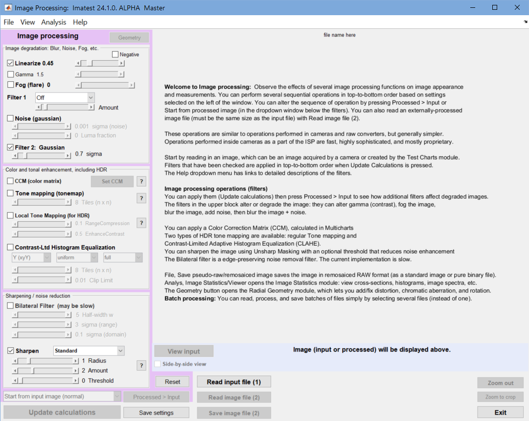 Image Processing opening window. Click on image to view full-sized.
Read an input image file. Any type of image can be used. It doesn’t have to be a test chart. (1) is on the button because it’s the first step. You can crop the image now or later— the crop setting will be maintained.
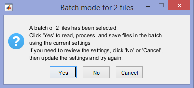 Read and process batches of files If several files are selected, they will be read, processed, and automatically saved in a batch using the stored settings. (Most of the outputs won’t be visible, but of course you can open the saved files for examination.) The dialog box shown on the right will open after you select the files. Files named root_file_name.ext will be saved as root_file_name–ext-improc.png.
Before running a batch of images you should run a single images to be sure you have the correct settings. Note that the batch calculations are not optimized for speed, so batch processing, which typically takes several seconds per image, is not suited for high volumes of images.
Next, either
- Read another file, which should have the same scene content but different image processing from the first image. This is done by pressing Read image file (2). Examples include two images captured at different ISO speeds, two images saved with as different file types (e.g, different levels of JPEG compression), or an in-camera JPEG and an externally-converted JPEG).
- Process the image by selecting settings in the left column, then pressing Update calculations. Blocks that are checked in the left column are performed in top-to-bottom order.
When either of these operations has been performed all the buttons are enabled. You can quickly toggle between the original and processed image, display measurements comparing the two, or save the processed image. When you are ready you can run another set of image processing operations,starting from either the original image or the processed image.
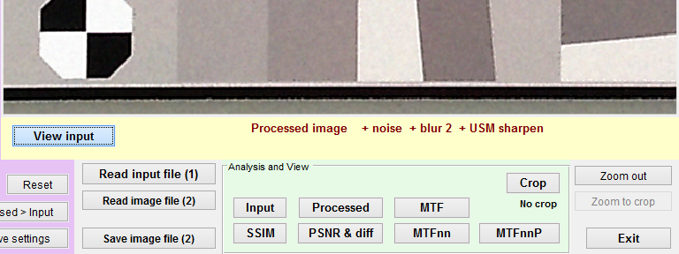
Here is the Image Processing display for an image of a Spilled Coins chart (cropped). The input image (of good quality, but with some visible noise) is displayed.
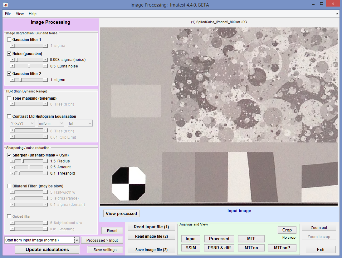 Image processing window showing Spilled Coins input image
Zoomed in (for display-only)
Cropping and zooming— There are two distinct types of crop/zoom operation: zooming for display-only and cropping for calculations (as well as display).
- Zooming (cropping for display-only) is performed by the standard Matlab procedures: clicking on the image (to zoom in), dragging and clicking to select a region, or by double-clicking (to zoom out). These does not affect calculations such as MTF.
- Cropping for calculations as well as display is performed by pressing the Crop button in the Analysis and View area below the image. This brings up the standard Imatest coarse and fine crop windows. This approach affects calculations such as the MTF curve (which is image-dependent for several processing blocks) or the mean SSIM calculation (though the detailed SSIM plot is unaffected). Pressing the Crop button enables the Zoom out and Zoom to crop buttons on the lower-right of the window. To remove the crop, press the Crop button and select the entire image.
Image processing blocks
As we indicated, image processing takes place from the top to the bottom of the left column when Update calculations is pressed. Some of the enhancement steps, particularly Unsharp Masking, are routinely performed in cameras for JPEG processing. They are not performed when raw images are demosaiced in Imatest (using dcraw or Generalized Read Raw).
Here is a list of the processing functions currently available. Most are standard Matlab functions; one is a user-supplied function from the Mathworks File Exchange. Nonuniformity or nonlinearity are indicated in bold blue. Nonuniform or nonlinear operations are not recommended for image information metric calculations.
| Processing block | Description | Function: described in link |
| Linearize | Linearize the image (remove the gamma encoding) at the start of the calculations. Operations are applied to the linearized image, then gamma encoding is reapplied. Most useful with standard sharpening (the 2D version of the 1D sharpening described on the Sharpening page. Not for USM. | |
| Gamma | (Not exactly a degradation) Add or remove gamma encoding from an image. There are cases where you may want to remove gamma encoding, apply filters, then reapply gamma encoding (in a second pass). The gamma value is relative to an assumed input gamma of 1. imageout = imageingamma | |
| Negative | Invert the image, i.e., turn it into a negative (added in 5.0.4). | |
| Image degradations: Often found in images prior to processing. Operations are generally linear. | ||
| Fog (flare) | Fog the image: equivalent to adding flare light or veiling glare. imageout = sqrt(fog + (1-fog)*handles.imagein2) |
|
| Gaussian Filter 1 | Blur the image (before applying noise). This simulates lens blurring. | imgaussfilt: 2-D Gaussian filtering of images with parameter sigma. |
| Noise (Gaussian) | Add noise to the image. Will be filtered by Gaussian Filter 2. | imnoise: Add noise to the HSV V channel. Parameters sigma [] and Luma noise []. |
| Gaussian Filter 2 | Blur the image + noise (after applying noise). This affects the noise spectrum. The spectrum for σ = 0.5 is similar to output of demosaicing (in raw conversion), which decreases noise from 1 to 0.5 at Nyquist. | imgaussfilt: 2-D Gaussian filtering of images with parameter sigma. |
| Tonal enhancement: Correct colors or apply one of three tone mapping algorithms, used for displaying High Dynamic Range (HDR) images. Tonal response may be highly nonlinear. | ||
| Color Correction Matrix (CCM) | 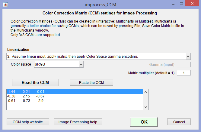 Apply a Color Correction Matrix (CCM), which can be calculated and saved in Multicharts. Saved values are entered when Image Processing is opened. The Set CCM button to the right of the CCM checkbox opens a window (shown on the right; click on thumbnail to view full-sized) that lets you set up the matrix (read it from a file or paste it from the clipboard and select options (linearization, etc.)). Apply a Color Correction Matrix (CCM), which can be calculated and saved in Multicharts. Saved values are entered when Image Processing is opened. The Set CCM button to the right of the CCM checkbox opens a window (shown on the right; click on thumbnail to view full-sized) that lets you set up the matrix (read it from a file or paste it from the clipboard and select options (linearization, etc.)). |
Color Correction Matrix describes the CCM, which is calculated in Multicharts. |
| Tone mapping | Render high dynamic range (HDR) image for viewing: convert a high dynamic range image to a lower dynamic range image, suitable for display, using a process called tone mapping. Tone mapping is a technique used to approximate the appearance of high dynamic range images on a display with a more limited dynamic range. Nonuniform and nonlinear | tonemap: Render high dynamic range image for viewing |
| Local tone mapping | Alternative tone mapping algorithm for HDR images using Laplacian filtering. Has a different set of adjustments. Produces different results (more saturated images). Nonuniform and nonlinear | localtonemap |
| Contrast-Limited Histogram Equalization | CLAHE operates on small regions in the image, called tiles, rather than the entire image. Each tile’s contrast is enhanced, so that the histogram of the output region approximately matches the histogram specified by the ‘Distribution’ parameter. The neighboring tiles are then combined using bilinear interpolation to eliminate artificially induced boundaries. The contrast, especially in homogeneous areas, can be limited to avoid amplifying any noise that might be present in the image. Nonuniform and nonlinear | adapthisteq: Contrast-limited adaptive histogram equalization (CLAHE) |
| Spatial enhancement: sharpening and/or noise reduction. Output depends on image content— may be highly nonlinear. | ||
| Sharpen USM (Unsharp Mask) |
Sharpens the grayscale or RGB input image using the unsharp masking (USM) method. Most visible on edges. USM works by subtracting a gaussian blur function from the original image. If threshold > 0, low-contrast regions may not be sharpened. See Wikipedia. This function is not linear. It caused some inconsistencies with the image information metrics. Designed to work directly on images, which should not be linearized. Nonlinear (a surprise; not indicated in MATLAB documentation) |
imsharpen: Unsharp Masking (USM) |
|
Sharpen (New in |
Sharpens the grayscale or RGB input image using a 2D version of the 1D sharpening method described in the Sharpening page. Most visible on edges. It works by subtracting an amplitude-reduced replica of the original image, arranged on a circular locus with radius R, from the original image. To maintain linearity, Linearize should be checked. This causes the image to be linearized (gamma-encoding removed) at the start of the calculations. Then sharpening is applied to the linearized image, then gamma encoding is reapplied. Recommended for testing the effects of sharpening on image information metrics, such as SNRi or Edge SNRi. Because standard sharpening is not a MATLAB function, we include more explanation in the box below. |
Custom function. Either USM or Standard sharpen can be applied (but not both). |
| Bilateral filter |
Nonuniform |
bfilter2 (from the Mathworks File Exchange): |
A complete (though elementary) Image Processing pipeline can be simulated by reading a raw or minimally processed image (demosaiced by ReadRaw), then applying operations such as Color Correction Matrix (which also applies a gamma curve), sharpening, and a bilateral filter (a simple example— there are many options).
|
Sharpening (standard; not USM) is an Imatest (not a MATLAB) function, designed to maintain linearity. As we mentioned above, this is a 2D version of the 1D sharpening method described in the Sharpening page. It was created when we were trying to determine if USM, which is implemented with the MATLAB imfilter function, is nonlinear (it is). It is also closer to typical camera sharpening than USM, which is more computationally intensive. For sharpening radius R and amount A, define ksharp = A/(A+1). The filter kernel is a 2R+1×2R+1 matrix H (units of pixels), calculated by (1) setting each entry at a distance r from the center to H(r) = max(|R-r|,0), (2) setting H = H/∑H, then setting the entry at the center, H(R+1,R+1) = 1. For a filter with Radius = 2, Amount = 3 (strongly sharpened), the 5×5 kernel is -0.0092 -0.0409 -0.0535 -0.0409 -0.0092 Standard sharping should be used with Linearize γ for gamma-encoded images. It is a linear operation (as long as excessive sharpening doesn’t saturate the image). |
Utilities
Several utilities are available in the dropdown menus at the top of the image processing window. (There is little room for added buttons in the window.)
| File | Display and/or Save screen | Display the screen in an image viewer (Irfanview recommended) and optionally save it. This function is in several interactive modules. |
| Save image | Save the processed image. Normally images will be saved in full precision (except if 8-bit max (below) is checked). | |
| Save pseudo-raw/remosaiced image | Save the image in a pseudo-raw (remosaiced) or special format, including Bayer, RCCC, or specific channel can be selected. Many options. See Synthetic RAW images. | |
| Save image as monochrome | Save the image (which may be color) as a monochrome image. | |
| Swap Endian (16, 32-bit input) | Swap the order of bytes within pixels (useful in rare instances where they are incorrect) | |
| Save image files with 8-bit max precision | Unchecked (off) by default. If set, images will be saved in 8-bit precision. (This should normally be unchecked). | |
| Save image as HDR | Save the image in HDR (High Dynamic Range) format | |
| View | Colorbar (grayscale or color) | Grayscale or color: Used in SSIM and PSNR displays. The colors in the color bar can be changed in Options II. |
| Crop | Lets you select a crop for image analysis operations (MTF, SSIM, etc.) Same as the Crop button in the Analysis and View area. | |
| Analysis | Most functions duplicate buttons in the Analysis and View section, but there are several additions. | |
| Image Statistics | Call the Image Statistics module for viewing image statistics such as histograms and cross-section profiles. | |
| Radial Geometry | Call the Radial Geometry module, which can return an image with added or corrected optical distortion, lateral chromatic aberration, and/or rotation. | |
| OCR | Optical Character Recognition using Matlab’s OCR function | |
| Detect faces | Uses the Matlab CAMShift routine, described below. | |
| Detect people | Uses the Matlab detectPeopleACF routine, described below. Less effective than Face detection. | |
| Help | Open web pages with descriptions of various image processing blocks. | |
Results display and analysis
The display is controlled by buttons below the image or by the Analysis dropdown menu. You can choose between a visual display of the Input or Processed image or a calculated display (an analysis comparing the input and processed images).
| Input | Display the input image (1) |
| Processed | Display the processed image (2) |
| MTF | Display the MTF of the processed / input image as a function of spatial frequency. Sensitive to cropping. |
| MTFnn | Display a polar plot of MTF70-MTF10 (spatial frequencies where MTF is nn% of low frequency value) |
| MTFnnP | Display a polar plot of MTF70P-MTF10P (spatial frequencies where MTF is nn% of peak value) |
| SSIM | Display the Structural Similarity Index, which is discussed in detail on the page for the SSIM module. Better correlated to visual differences (degradations) than PSNR. |
| PSNR & DIff | Display the Peak Signal-to-Noise Ratio and the difference between images. |
| OCR | Optical Character Recognition results using Matlab’s OCR function |
| Detect faces | Face detection results using the Matlab CAMShift routine. |
| Detect people | People detection results using the Matlab detectPeopleACF routine, described below. Less effective than Face detection. |
The View input button on the left, just below the image, toggles between View input (when the processed image is selected) and View processed (when the input image is selected). This enables rapid visual comparison of the two images. The zoom setting is preserved when you switch images. The View input/processed button performs the same functions as the Input and Processed buttons in the Analysis and View area. The other buttons in this area display calculated results.
SSIM displays the Structural Similarity Index, which is discussed in detail on the page for the SSIM module. It’s primary use is in measuring the visible effects (i.e., degradation) of image compression from saving files (for example, JPEGs of varying quality) and from data transmission.
MTF (Modulation Transfer Function) calculates the transfer function between the Processed and Input images using a 2D Fourier transform similar to the calculation in the Random module, but with one important difference. Unlike the Random module, where the scaled Power Spectral Density in gray areas to the left and right of the active area (the random/Spilled Coins/Dead Leaves pattern) is subtracted from the total power spectral density of the active area to remove most of the noise, there is no noise reduction. Hence this MTF measurement is extremely sensitive to noise.
 MTF for noisy Gaussian-filtered image after Unsharp Masking
|
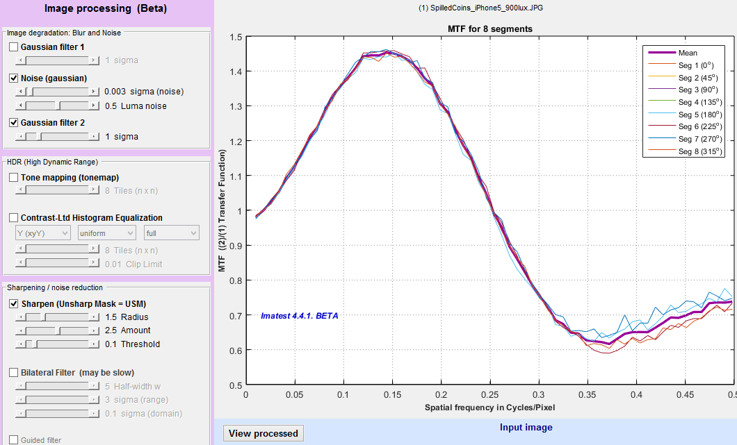
The high frequency rolloff is the effect of Gaussian filter 2, which is applied after the noise has been added (and hence shapes the spectral power of the noise). You can see the MTF for Unsharp Mask (USM)-only (in this case with Radius = 1.5 and Amount = 2.5) by unchecking Noise (gaussian) and Gaussian filter 2 in the Image Processing area to the left of the image, then pressing Update calculations. Unsharp Masking has a different spectral response from the type of sharpening described in the Sharpening page: It’s response is not cyclical. It rises to an asymptotic level of Amount+1 and stays high. This is a good example of how Image Processing can be used to explore the effects of processing blocks on both appearance and measurements. |
 MTF for USM (Unsharp Mask: Radius = 1.5; Amount = 2.5) MTF for USM (Unsharp Mask: Radius = 1.5; Amount = 2.5) |
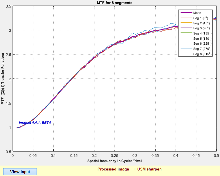
Side-by-side view
The side-by-side view allows you to compare the input and processed images side-by-side, i.e., right next to each other. Click the Side-by-side view checkbox just below View input or View processed (on the left, below the image). When the box is first checked the two images are displayed in their entirety. If you crop one, the other will have the identical crop. This makes for meaningful comparisons.
 Side-by-side view of Dead Leaves chart. Noise, Bilateral filter, and USM added on the right.
When Side-by-side view is enabled, the Analysis and view section on the bottom (which contains MTF, SSIM, etc.) is disabled. Uncheck to re-enable it.
Remosaicing (undemosaicing)
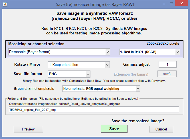 By clicking File, Save pseudo-raw (undemosaiced) image (after a file has been read), you can save the image in a synthetic Bayer RAW format as well as one of several other formats. The output can be a standard image file format or pure binary. A dialog box opens that allows a number of options.
Mosaicing or channel selection None (Normal color file output), Remosaic (Bayer format), RCCC (Red-Clear-Clear-Clear): R bright, RCCC (Red-Clear-Clear-Clear): R = C/3, Monochrome (Y = luminance), Monochrome (mean: equal weights), Red, Green, Blue. For remosaicing (creating Bayer RAW files), Remosaic (Bayer format) would be selected.
Red in RmCn lets you select one of the four Bayer configurations.
Gamma adjust lets you adjust the gamma of the output curve. Keep it at 1 for no change. Use 2 (or 2.2) to go from a typical color space gamma to linear (gamma = 1).
Save file format lets you select a standard image file format (PNG, JPG (90% quality), TIF (large), BMP, Binary 8-bit, or Binary 16-bit. The binary files can be read into Generalized Read Raw.
Green channel emphasis lets you emphasize the green channel so that the synthetic RAW image resembles actual raw images, which typically are strongest in green. Several Blue/Red levels are available.
When you select Save, a dialog box lets you select the location and file name. The default is root_file_name_png (with the selected extension).
Optical Character Recognition (OCR)
|
OCR has been added in Imatest 5.0, using Matlab’s OCR function, which is an implementation of Tesseract-OCR. To use it,
This opens the OCR window and performs a text recognition operation on the crop of the image. Results for the sample image on the right (mildly degraded with Noise (gaussian) = 0.002; Gaussian filter 2 = 0.7) are shown below. You can download this image and experiment with to see how various degradations and enhancements affect OCR performance. Be forewarned. Matlab’s OCR performance is not impressive. Text that appears to be quite readable does not do well, especially for font sizes under 12 points. Performance is comparable to several free or low-cost OCR programs such as gImageReader (a GUI front-end for Tesseract-ocr) and TopOCR. |
The left side sample image consists a set of characters (QWERTYUIOPASDFGHJKLZXCVBNM1234567890) of different sizes ranging from 20 to 7 points in normal, bold, and negative bold Calibri font. These are characters used in automotive license plates. The file (here) was created in Microsoft Word. The remainder of the image is a portion of the Enhanced eSFR ISO chart, with wedges and two high contrast squares. These can be used to correlate MTF measurements with OCR performance. |
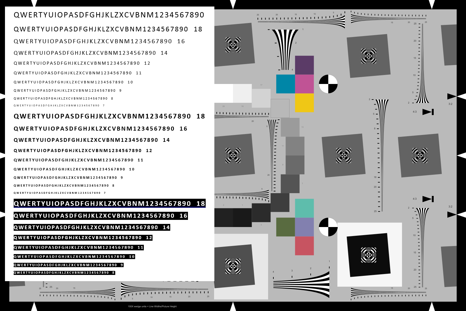 Sample image: Click for a
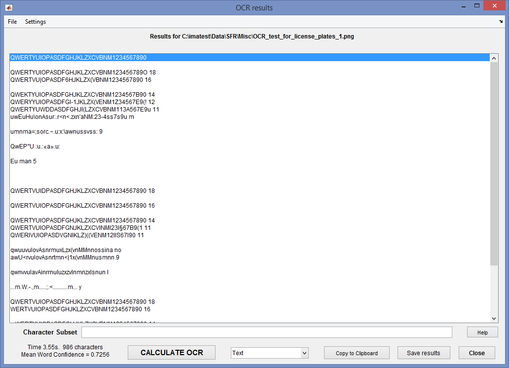 OCR window, showing results for mildly-degraded crop of the sample image
OCR Settings
Character Subset Results can be improved by entering a character subset to limit the valid output characters (all characters are allowed if Character Subset is blank), then pressing CALCULATE OCR. For the sample image, the subset consists of Latin capital letters and numbers (typical of automobile license places). It makes only a small improvement.
QWERTYUIOPASDFGHJKLZXCVBNM1234567890
Standard OCR does not work very well with license plates. Several license plate detection routines are available in the Matlab File Exchange. We may add one or two if they work well and the license allows.
Display Text (shown) is the default. You can also select Confidence & words, which shows the Word Confidence and individual word. Here are a few lines from the display.
0.8545 QWERTYUIOPASDFGHJKLZXCVBNM1234567890
0.8361 QWERTYUIOPASDFGHJKLZXCVBNM123456789O
0.9018 18
0.7842 QWERTVU|OPASDF6HJKLZX(VBNM1234567890
0.8339 16
0.7468 QWEKTYUIOPASDFGHJKLZXCVBNM1234567B90
0.8254 14
0.7252 QWERYYUIOPASDFGI-1JKLZX(\/ENM1Z34567E9(!
0.7784 12
0.5777 QWERTYUWDDASDFGHJI(LZXCVBNM113A567E9u
0.6549 11
0.6276 uwEuHu\onAsur:.r<n<.zxn’aNM:23-4ss7s9u
0.7658 m
Copy to clipboard You can copy the current display into the clipboard for use in text editors or other applications.
Save results saves the current display.
Variable or fixed width font can be selected in the Settings dropdown menu.
Face and People detection
Face and people detection can be called from the Analysis dropdown menu. Both currently use the Matlab default settings. (We may add an options window in the future.) See
Face Detection and Tracking Using CAMShift and detectPeopleACF
Face detection works somewhat better than people detection. Here is an example, using an image shamelessly stolen from http://epaperpress.com/portfolio/columbia.html. The soggy author of Imatest is on the left. Click Update Calculations to remove the annotations (to reset the image).
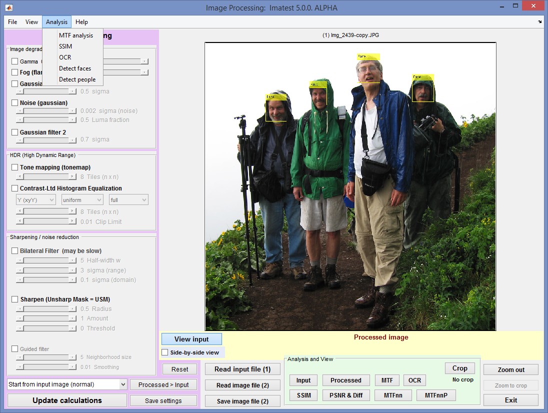 Example of Face Detection (Imatest author on the left)
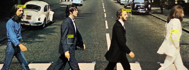 Face detection works pretty well much of the time, but seriously… How can you miss Paul and John?