Introduction – Flowchart – Math – Linearization – Calculating in Color/Tone Interactive
Optimization steps – Reference files and “Gold Standard” – Saturation
Applying the matrix – 1. in Color/Tone 2. in Image Processing 3. externally with program code
Color Accuracy Solutions
Introduction
Color/Tone Interactive and Auto can calculate a color correction matrix (CCM) from an image of a color test chart that has at least 9 distinct color patches. 3×3 CCMs are generally recommended, but 4×3 is supported. Excellent results can usually be achieved with the inexpensive, widely-available 24-patch X-Rite Colorchecker. The CCM can be applied to images to achieve optimum color reproduction, which is defined as the minimum mean squared color error between corrected test chart patches and the corresponding reference values, which can be
- standard (published) reference values,
- measured with a spectrophotometer, or
- saved L*a*b* values from a “gold standard” image (when the intent is to match images).
The default color error parameter is the mean of (ΔE 2000)2 (or (ΔE 94)2, which is very similar), calculated for all patches where 5 ≤ L* ≤ 98 ( where L* is defined in CIELAB color space) and each of the R, G, and B channels are less than 99% of the maximum value (i.e., the patch is unsaturated). Nonlinear optimization is used to calculate the matrix.
The CCM can be used in the Input Device Transform (IDT) of cinema workflows, such as the Academy Color Encoding System. It can be used to achieve consistent color when several different cameras are used to capture a scene.
In setting up color matrix calculations, it is very important that the image be properly linearized because the matrix operates require linear R, G, B values. Several linearization options are available for different image encodings.
Sequence of operations — The Flow chart
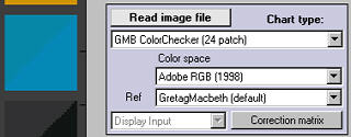
Quick summary: Start with an uncorrected image of a color chart. It doesn’t need to have a color space associated with it. Raw images work best. Examine its tonal response curve to determine what linearization is needed, then select the settings (including the (target) color space and reference file). Press Correction matrix to run the optimizer that finds the matrix with the minimum sum of the squares of color errors.
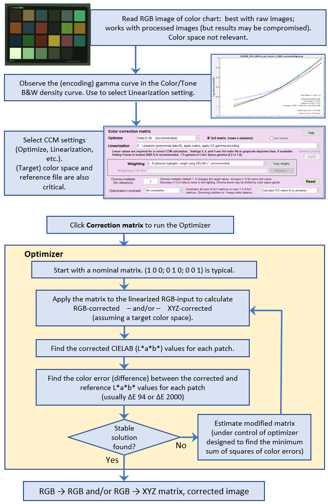
Color correction matrix (CCM) calculation workflow
The MathThe matrixColor images are stored in m x n x 3 arrays (m rows (height) x n columns (width) x 3 colors). For the sake of simplicity, we transform the input color image to a k x 3 array, where k = m x n. The Original (uncorrected and linearized* input) pixel data \(O\) can be represented as \( O = \begin{bmatrix} O_{R1} & O_{G1} & O_{B1} \\ O_{R2} & O_{G2} & O_{B2} \\ & … & \\ O_{Rk} & O_{Gk} & O_{Bk} \\ \end{bmatrix} \) where the entries of row i, \([O_{Ri}\quad O_{Gi}\quad O_{Bi}]\) , represent the normalized and linearized* R, G, and B levels of pixel i. The transformed (corrected) array is called \(P\), which is calculated by matrix multiplication with the color correction matrix, \(A\). Imatest allows you to choose two different forms of \(A\), either 3×3 or 4×3. (4×3 is no longer recommended; it may be deprecated unless we hear from users.) \(P=O \, A\) (\(A\) is a 3x3 matrix) Each of the R, G, and B values of each output (corrected) pixel is a linear combination of the three input color channels of that pixel. \(P = \begin{bmatrix} P_{R1} & P_{G1} & P_{B1} \\ P_{R2} & P_{G2} & P_{B2} \\ & … & \\ P_{Rk} & P_{Gk} & P_{Bk} \end{bmatrix} = \begin{bmatrix} O_{R1} & O_{G1} & O_{B1} \\ O_{R2} & O_{G2} & O_{B2} \\ & … & \\ O_{Rk} & O_{Gk} & O_{Bk} \end{bmatrix} \begin{bmatrix} A_{11} & A_{12} & A_{13} \\ A_{21} & A_{22} & A_{23} \\ A_{31} & A_{32} & A_{33} \end{bmatrix}\)
The goal of the calculation is to minimize the difference (in some chosen metric, described below) between \(P\) and the reference array (the ideal chart values) \(R\). The initial values of \(A\) (the starting point for optimization) for the 3x3 and 4x3 cases are, respectively, \[ A_{(3\times3)} = \begin{bmatrix} k_R & 0 & 0 \\ 0 & k_G & 0 \\ 0 & 0 & k_B \end{bmatrix} \; ; \scriptstyle{\qquad A_{(4\times3)} = \begin{bmatrix} k_R & 0 & 0 \\ 0 & k_G & 0 \\ 0 & 0 & k_B \\ 0 & 0 & 0 \end{bmatrix}} \] where \( k_R = \mathrm{mean}(R_{Ri})/\mathrm{mean}(O_{Ri}) \) \( k_G = \mathrm{mean}(R_{Gi})/\mathrm{mean}(O_{Gi})\) \( k_B = \mathrm{mean}(R_{Bi})/\mathrm{mean}(O_{Bi})\) for reference array \(R\) and original array \(O\) where the mean is taken over all \(i\). |
|
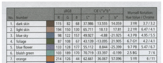
Color/Tone requires a reference array R for each chart type. (Sometimes— for example with the X-Rite Colorchecker— more than one is available). R typically contains CIELAB (L*a*b*) values, which can be converted to RGB or used to calculate the color difference metric (ΔE, ΔC, …). You can
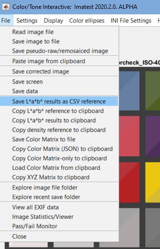
In the Color/Tone Interactive module, you can press File, Copy L*a*b* reference to clipboard to get the current reference values. A few values for the Colorchecker are shown on the right. A small crop from the X-Rite page is shown below. |
37.31 13.39 14.58 64.37 18.05 17.05 49.62 -1.162 -22.16 43.35 -14.62 22.86 55.18 12.16 -24.57 70.67 -31.91 0.08472 62.11 33.4 55.77 40.05 16.27 -44.37 50.06 48.12 15.6 30.21 24.4 -20.88 71.52 -28.38 58.85 70.96 14.79 67.25 29.15 21.68 -48.74 54.35 -42.65 32.87 41.82 50.35 27.36 (24 rows total) |
Linearization
Although most standard (non-HDR) image sensors are linear up to the point where they saturate, many image files are highly nonlinear. Imatest deals with two broad types of image file.
- “Raw” files, which are converted from the sensor output without applying a gamma curve (and often little or no signal processing, i.e., sharpening, noise reduction, white balance, etc.) These files are linear with gamma close to 1 (often somewhat below 1 because of lens flare and on-sensor signal processing (adding pedestals)). RAW files are preferred for CCM calculations because the processing used to obtain gamma-encoded interchangeable files can cause some information loss (especially with sRGB color space).
- Files designed to be interchangeable and to be displayed at a specified gamma ( γ ), where display luminance = pixel level γ. (represented to the tonal response curve, log luminance = γ × log pixel level).
These files generally have a color space associated with them (which may or may not be embedded in the file). Gamma = 2.2 for the most commonly used color spaces (sRGB (approximately 2.2) and Adobe RGB (1998)).
When cameras encode images (a part of the RAW conversion process), they apply a tonal response curve (log pixel level vs. log exposure) that is an approximate inverse of the display curve: the slope may vary considerably from 1/γ, and it often includes a “shoulder” (an area of reduced contrast) in the tonal response curve to minimize highlight burnout. The shoulder improves pictorial quality by making the response more “film-like”, but may reduce the accuracy of the CCM.
| The CCM calculation assumes that any image processing applied to the image is uniform, and that individual colors are not saturated. A good CCM cannot be calculated after local tone mapping has been applied. |
If the input image has been gamma-encoded it must be linearized prior to applying the correction matrix. Imatest has several linearization options, described below. Options 1 and 5-8 linearize the input image. 2-4 assume the input image is linear.
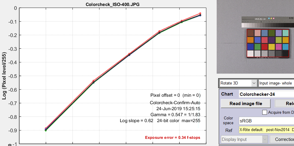
|
This particular curve has a gamma (average slope) of 0.547 and a response “shoulder”. Raw files, which work better with CCM calculations, typically have a slope (gamma) close to 1 and no shoulder. A reasonable (but far from perfect) Linearization setting is 7. Linearize input using gamma… with gamma set to 0.55 in the box below the linearization settings dropdown menu. Better results can be obtained with settings 5 or 9, which make no assumptions about gamma: they measure it from the grayscale patches in the image. 5 is adequate for RAW images (with gamma close to 1). |
Optimization steps
- Open the image to be used to calculate the CCM in Color/Tone (either Interactive or Auto).
- Select the settings, most of which are located in the Settings window.
The tonal response (including gamma) of the input image (as shown in the box above) is used to determine the appropriate Linearization option. If Color space gamma linearization is selected, OL = Ogamma. (where gamma (γ) is specified by the color space, e.g., 1/2.2 for Adobe RGB).
Be sure the correct Color space and Reference file are selected in the Color/Tone window. - Call the optimizer by pressing the Correction matrix button, which
- calculates a (temporary) corrected image TL = OL A.
- (Optionally) removes the linearization: T = TL(1/γ) using the color space gamma (γ).
- Finds the color error metric between T (converted into CIELAB, i.e., L*a*b* values) and the reference (ideal) array R. for each patch. The color error metric, selected in the Optimize dropdown menu, is one of the standard color error measurements: ΔE*ab, ΔC*ab, ΔE94, ΔE94, ΔECMC, ΔCCMC, ΔE00, or ΔC00, described here. ΔE00 (CIEDE2000) or ΔE94 are the recommended selections. [Before we added color difference ellipses to a*b* displays we were concerned that ΔE00 might contain small discontinuities that would affect optimization.] The ΔC errors are similar to ΔE with luminance (L*) omitted. They are not recommended because there is an interaction between the chroma (a* and b*) and luma (L*) components of L*a*b* color space, and chroma is actually less accurate when one of the ΔC values is selected.
- Adjusts A until a minimum value of the sum of squares of the error metrics (usually ∑(ΔE00)2 or ∑(ΔE00)2 for patches where 5 ≤ L* ≤ 98 is found, using nonlinear optimization.
- Reports the final value of A.
In applying A (generally outside of Imatest), a similar linearization should be used. A may be applied without linearization during the RAW conversion process, prior to the application of the gamma + tonal response curve.
There is no guarantee that A is a global minimum. Its final value depends to some extent on its starting value.
The Color correction matrix in Color/Tone
Options: Color matrix calculation options can be set by clicking Settings, Color matrix in the Color/Tone Interactive window or by pressing the button in the settings window. This brings up the dialog box shown below. The options are
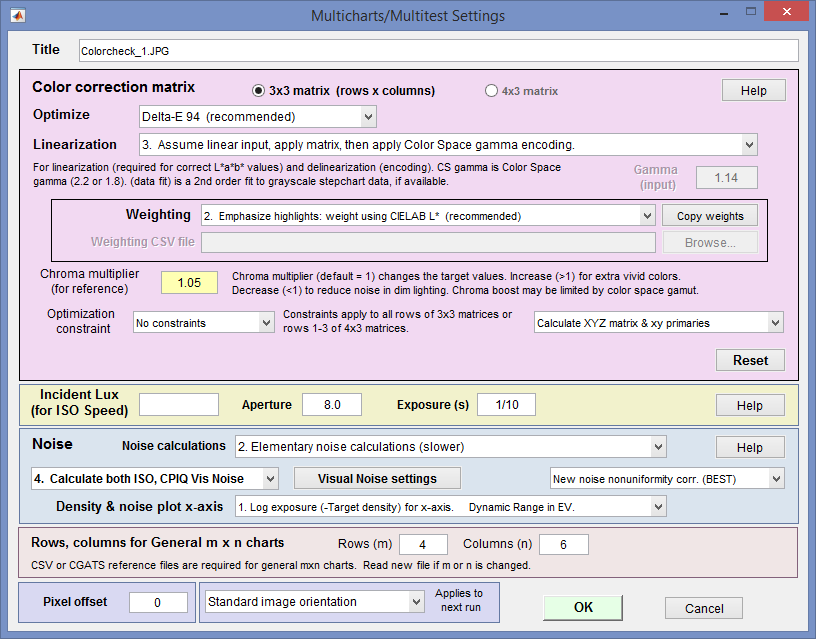 4×3 or 3×3 matrix: Color correction matrix size. 3×3 is generally recommended. 4×3 matrices include a dc-offset (constant) term that slows computations and rarely improves the results.
- Optimize: Select the color error parameter whose mean of squares over patches with L*>10 (nearly black for 95) is to be minimized. Choices include ΔE ab, ΔC ab, ΔE 94, ΔE 94, ΔE CMC, ΔC CMC, ΔE 00, and ΔC 00, described here. ΔE 94 or ΔE 2000 are recommended because they give less weight to chroma differences between highly chromatic (saturated; large a*2 + b*2 ) colors, i.e., they are closer to the eye’s perception than ΔE ab (the standard ΔE calculation: the geometrical distance between colors in L*a*b* space).
- Weighting: Set the weighting of the patches for optimization. Choices:
- 1. Equal weighting [default] Patches are equally weighted. May not be the optimum setting because highlight colors may be more visually prominent than shadow colors.
- 2. Emphasize highlights: weight according to CIELAB L* Give more weight to visually-prominent highlight patches. This is the default.
- 3. Strongly emphasize highlights: weight according to L*^2.
- 4. Read weighting from a CSV file If selected, the Copy weights, browse, and file boxes are activated. The CSV file should have the same number of weights (typically in the range of 0 to 1) as patches in the chart. The file may one value per line or m values per line on n lines, as long as m*n = the number of patches in the chart.
| Here is an example of weights for the 140-patch (10 rows x 14 columns) Colorchecker SG.
0,0,0,0,0,0,0,0,0,0,0,0,0,1 |
colormatrix_SG_numbers") Pressing the Numbers checkbox (on the right of the Color/Tone window) when a weight file has been entered and the CCM has been calculated displays both the patch number (the Colorchecker 24 replica section of the SG is shown) and the weights. This can help verify that the correct weights have been entered. Pressing the Numbers checkbox (on the right of the Color/Tone window) when a weight file has been entered and the CCM has been calculated displays both the patch number (the Colorchecker 24 replica section of the SG is shown) and the weights. This can help verify that the correct weights have been entered. |
- Linearization: Choose the method for linearizing the image prior to calculating the matrix. For most settings (all but 5, 6, and 9) you need to know the tonal response (encoding) of the input image, which can be linear (typical for raw images), gamma-encoded (using a manually-entered gamma ( γ ) or the gamma for the selected color space (sRGB, Adobe RGB, etc.)), or logarithmically-encoded. The response can be obtained from the B&W density plots for the grayscale portion of the chart. The equation for linearizing gamma-encoded color spaces is OL = O1/γ. The equation for gamma encoding (after the CCM has been calculated) is O = OLγ.
For settings 5, 6, and 9 you don’t need to know how the image has been encoded. The linearization parameters are determined by a polynomial fit to the grayscale data (to grayscale patch levels L for settings 5 and 6 or log10(L) for setting 9), using the Matlab polyfit and polyval functions.
| Setting | Comments | Linearization equation: Linear level = |
| 1. Linearize input (CS gamma), apply matrix, then apply CS gamma encoding | A reasonable choice for images encoded in a standard color space (CS). | input1/(CS gamma) |
| 2. No linearization: apply matrix to input pixels | For experimentation and for images that start and remain linear. Not for gamma-encoded images. | input |
| 3. Assume linear input, apply matrix, then apply CS gamma encoding | For images that are not gamma-encoded (near linear), but need to be converted into a color space. Color space (CS) gamma is not applied in converting the input RGB image to L*a*b*. | input |
| 4. Assume linear input & output (gamma = 1 throughout) | No linearization or gamma encoding. Color space gamma is not applied in converting between RGB and L*a*b* spaces. (Same as 2) | input |
| 5. Linearize input (data fit), apply matrix, apply CS gamma encoding (fairly accurate) | Linearize the image using a third order polynomial fit P (Matlab polyfit function) to grayscale patch pixel levels L. Calculate the CCM, then encode with the Color Space gamma. This often gives good results. | polyval(P,input), where P is a third-order polynomial fit to L. |
| 6. Linearize input (data fit), apply matrix, then delinearize (data fit) | Same as 5, except that after optimization the image is restored to the original tonal curve. | Same as 5. |
| 7. Linearize input using gamma (below), apply matrix, then apply CS gamma encoding | Manually enter the gamma, which can be obtained from the B&W density plot if the color chart has a grayscale pattern. This produces excellent results in the frequent cases where the measured gamma differs from the expected color space gamma or 1 (for linear raw conversion). This setting is particularly useful when gamma of the input image differs from the standard color space gamma (often 1/2.2) or linear (1). | input1/gamma |
| 8. Linearize using log slope (for Log ColorSpace, below), apply matrix, then gamma encode (CS) |
For logarithmic color spaces (sometimes used in cinema; never in still photography), which are characterized by the approximate encoding equation, O = max(1+A log10(OL), 0) and inverse (for linearization) OL = 10^((O-1)/A). A is Log slope, which is displayed in the B&W density & White Balance display in the Color/Tone Interactive module. Log-encoded color spaces have approximately straight line response when the Pixels vs. Input Density option (new in 4.0) is selected, while gamma-encoded spaces have approximately straight line response when the more traditional Log(Pixels) vs. Input Density option is selected. |
|
| 9. Linearize (gamma polynomial data fit), apply matrix, apply CS gamma encoding. | Linearize the image using a third order polynomial fit P to log10 of the grayscale patch levels L. Calculate the CCM, then encode with the Color Space gamma. This is a polynomial modification of gamma encoding. Recommended because (A) it requires no knowledge of input image encoding and (B) it provides the most accurate results for a variety of images. | polyval(P,log10(input)), where P is a third-order polynomial fit to log10(L). |
Note: For the Rec. 709 color space, which has allowable values between 16 and 235 (of 255), linearization maps 16-235 to the full 0-1 (internal) range and delinearization maps 0-1 back to 16-235. The image is displayed full range.
- Gamma (only enabled for Linearization setting 7: Linearize using input gamma…). Manually enter the value of gamma measured from a grayscale stepchart (which is included in most color charts and is displayed in the B&W density plot).
- Chroma multiplier (for reference) Normally 1. Increase it for more saturated colors; decrease it for less saturated colors. Sometimes results are improved by increasing it to 1.05 or even 1.1.
- Optimization constraint
- No constraints. This is the default and should only be changed with good reason.
- Rows sum to 1.
- Columns sum to 1. This maintains white balance.
- Calculation details Two types of calculation are available: (1) Direct RGBin to RGBout, and (2) RGBin to XYZ (indirectly to RGBout). Both use an optimizer: they start with a first guess, then the optimizer adjusts the values until a minimum value of the selected error metric is found.
- Calculate RGB matrix directly (original algorithm) Start with a guess for the RGBin to RGBout matrix, then find L*a*b*out from RGBout. Under control of the optimizer adjust the matrix so the color error (between L*a*b*out and the reference values (adjusted by the chroma multiplier if ≠ 1) is minimum.
- Calculate XYZ matrix and xy primaries (newer algorithm) Start with a rough guess for the RGBin to XYZ matrix (sRGB coefficients are used). Then convert to XYZ to L*a*b* and adjust the matrix under control of the optimizer until the selected error metric is minimized. When optimization is complete, convert XYZ to RGBout. Both RGB to XYZ and RGB to RGB matrices are calculated and included in the CSV and JSON output files.
- Reference file (in the Color/Tone Interactive window; not in the Color Matrix window) The reference file contains the ideal chart L*a*b* values, used for the optimization. Normally it contains colorimetrically-measured L*a*b* values for the chart patches. This is always the case for the Default values and typically the case for reference files, but reference files may contain different values if a special “look” is desired, as described in Matching images, below.
|
Acquire an image of the test chart
Framing — The chart does not need to fill the frame, especially with cameras that have significant light falloff— which is common in wide-angle lenses with strong barrel distortion. Most of the time (except for cameras with very low pixel count), putting the chart in the central third of the frame (measured linearly) is sufficient.
Background — Bright illumination should be avoided in the background, either in or near the frame, because it can cause flare light that fogs shadows, making it difficult to achieve accurate correction. The ideal background is a neutral (~18% reflectance) to dark gray, but background color doesn’t have much effect as long as no color correction is applied prior to the CCM calculation.
Image processing — If possible, image processing should be kept to a minimum prior to the CCM calculation. Adjusting the color and/or transforming the image into a color space reduces accuracy. (This is what the CCM does.) Local tone mapping should be avoided: it completely ruins the calculations.
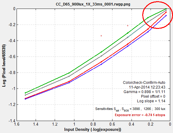
Saturation — Take care, if possible, to avoid saturating any of the patches. If patches are saturated, i.e., if any of the channels have an average pixel level above 99% of the maximum for the bit depth (e.g., 255 for bit depth = 8; 65535 for bit depth = 16) they will be omitted from the optimization and they will be labeled as Sat in the split view. It may not be visually obvious when a patch is saturated, especially if only one of the three channels is saturated (as shown below). Saturated patches tend to look very strange (see below) when the matrix is applied. (This may appear to be a bug, but it isn’t, as explained below.)
 Saturation Saturation
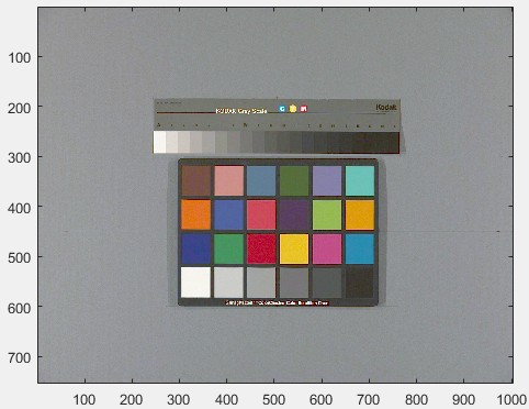
An image with a saturated patch (row 4, left) is shown on the right. It’s not obvious because only the green channel is saturated. This is apparent from the density response curve (from Color/Tone Interactive or Color/Tone Auto) shown below: the green channel is saturated at maximum exposure and the slope of the green curve drops just below maximum exposure. As a result of this, the green channel has a lower pixel level (relative to the other patches) than it would have had if it were not saturated. |
|
 |
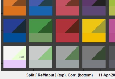 The corrected value of the saturated patch on the lower-left (shown on the bottom– it’s magenta!) is incorrect because the saturated green channel is lower than it would have been if the patch were not saturated. The corrected value of the saturated patch on the lower-left (shown on the bottom– it’s magenta!) is incorrect because the saturated green channel is lower than it would have been if the patch were not saturated. |
|
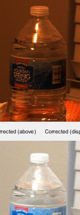
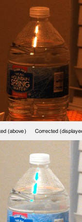
How Imatest handles saturated pixels (in Imatest 5.0+) When an R, G, or B pixel is saturated in the input file (has a value of 1 in the normalized data) it is kept at the saturated value after matrix is applied, i.e, the matrix is not applied to saturated (R, G, or B) pixels. This function is accomplished by the following line from the sample code below. correctedRGB(linearRGB==1) = 1; The images on the right show the results of this correction. The cyan highlight on the water bottle on the lower-left is the result of uncorrected saturation. The CCM has been applied to the lower images. A similar procedure is applied to cameras. It doesn’t (and can’t) give perfect results at the boundaries of saturated areas, which often display “purple fringing”. (The explanation in Wikipedia is incorrect. I may try to fix it.) |
|
To calculate the color correction matrix,
-
Open the image with Color/Tone Interactive or Color/Tone Auto.
-
Determine the Linearization setting from the density response curve in the B&W density display.
-
Set the Color matrix settings, paying special attention to the linearization, which should be consistent with the B&W density display.
-
Select the reference file, which contains the target values for color-correction. Most of the time the standard default values are used, but you can enter a reference file created from spectrophotometer measurements or by saving the L*a*b* values of a good (“gold standard”) image.
-
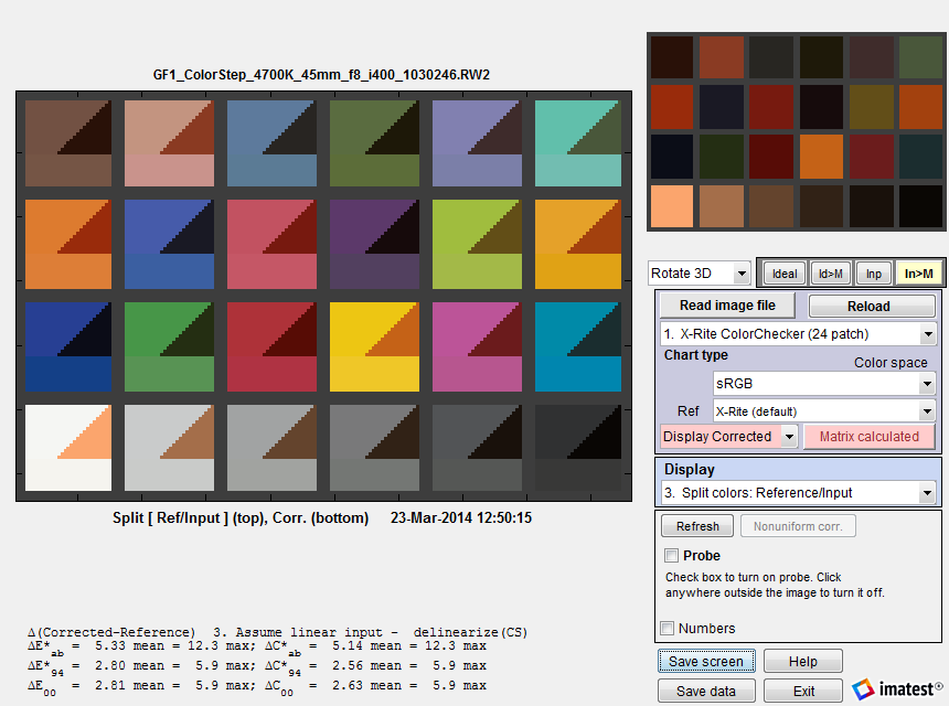
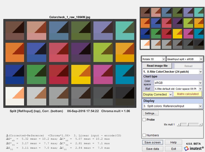
Press the button, shown on the right. The display will change, as shown below: Ideal (reference) colors remain on the upper-left of each patch, input colors remain on the upper right, and corrected colors are now displayed on the bottom. The input image (from our archive) has relatively poor white balance. The improvement is quite dramatic.
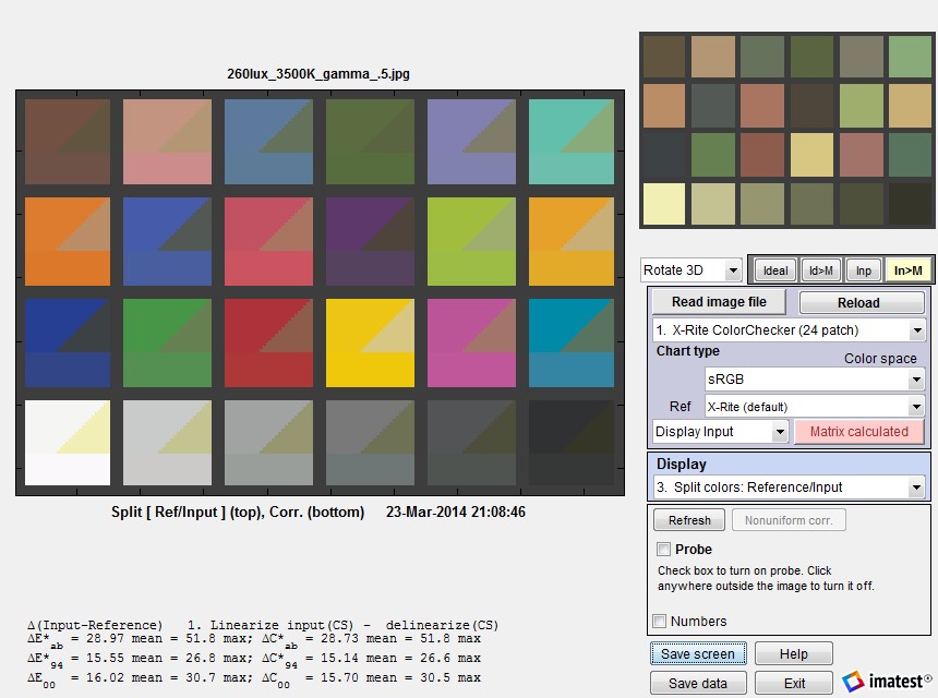 Split view, showing reference, input, and corrected patch colors. The dropdown menu that shows
Display input (on the right) can be changed to Display corrected to get [Corrected – ideal] statistics.
The button changes to , highlighted with a pink background. The correction matrix cannot be recalculated until an image property changes (new image, color space, reference file, or color matrix setting). The Display input (or Corrected) dropdown menu, immediately to its left, is enabled. You can choose one of two selections.
| Display input | Color differences (input − ideal) are shown in most displays, and [Input − ideal] Color differences are shown in the text in the lower left. Two displays are unaffected by this setting: Pseudocolor color difference and Split colors, where (corrected − ideal) is shown on the bottom. |
| Display corrected | 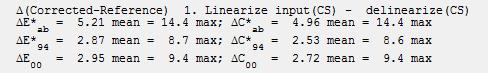 Color differences (corrected − ideal) are shown in most displays, and [Corrected − ideal] Color differences are shown in the text in the lower left. Here are the corrected color differences for the above case. Color differences (corrected − ideal) are shown in most displays, and [Corrected − ideal] Color differences are shown in the text in the lower left. Here are the corrected color differences for the above case. |
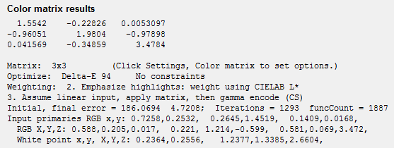
The EXIF data and Color matrix display contains a summary of results.
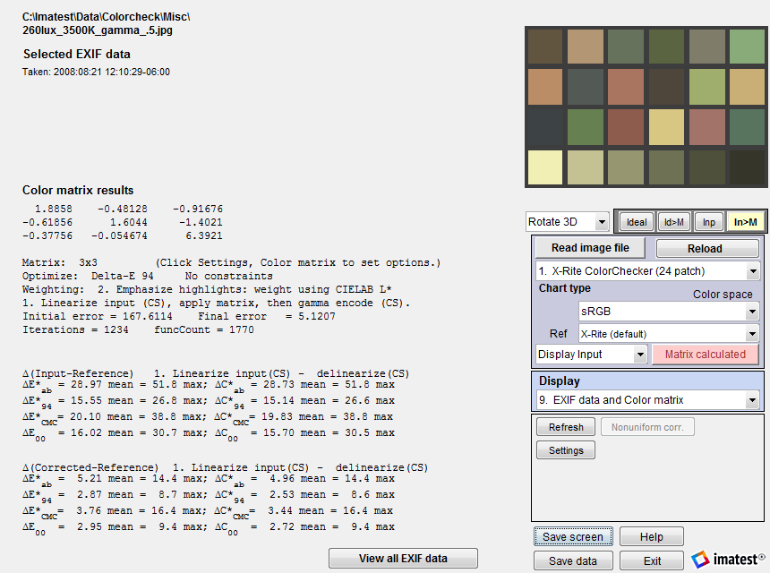 Exif and Color matrix view
The color correction matrix, results summary, and both [input – ideal] and [corrected -ideal] color difference summaries are shown. The initial and final error numbers shows how much the selected metric (in this case the sum of squares of Delta-E 94 for all patches with L*>10 and L*
Raw image results
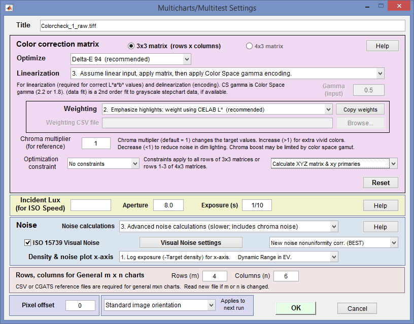
Here is an example of Color matrix optimization for a raw image. The original image was acquired as a raw (RW2) image (a JPEG was also acquired for reference) from a Panasonic GF1 Micro Four-Thirds (mirrorless interchangeable lens) camera, and converted using dcraw with Manual settings, Normal RAW conversion, Output gamma = 1.0 (Linear), Auto white level off (unchecked), White Balance = None, Output color space = RAW. These settings applied no image processing other than demosaicing.
The file was almost perfectly linear: the tonal response curve was a straight line with gamma = 1.01. Linearization option 3 (Assume linear input, apply matrix, then apply CS gamma encoding.) was selected.
The output is nearly perfect; about as good as it can get for a 3-color sensor. This is typical of what you might expect working from well-characterized raw images. We recently (May 2014) tested the calculation with four cameras that have RAW output (Panasonic Lumix LX7 and G3, Canon EOS-6D, and Nikon D800E) under six different lighting conditions (2700K and 5000K LED, 3500K and 5000K CFL, standard (2700K) incandescent, and 4700K (measured 4000K) SoLux (dichroic-filtered) halogen lamps), and we achieved remarkably consistent color-corrected images.
 Results from a linear raw file (gamma = 1; no color correction)
 x,y and X,Y Z primaries Color/Tone Interactive and Color/Tone Auto can calculate the x,y and X,Y Z primaries of the input (camera) color space, display them (the bottom three lines on the right), and save them in CSV and JSON output files. This calculation works best when the input image is linear (converted from raw without a gamma curve) or in ACES color space. It can be useful for calculating signal processing coefficients. Note that the x,y primaries are unrelated to the color gamut of the camera. These primaries are the the x and y values corresponding to R,G,B = {max,0,0}, {0,max,0}, [0,0,max}, which are unattainable in practice because of color crosstalk in the sensor and are often outside the spectral locus of real colors.
|
How good can color differences (ΔExx and ΔCxx) be? They can’t be perfect because the spectra of the color filters in trichromatic (three-color) cameras (approximately Red, Green, and Blue; RGB), is different from the filters in the human eye (approximately Yellow-Orange, Green, and Blue). Cameras do not duplicate the human eye because colors would have to be transformed to RGB to get good color reproduction, and this would badly degrade the Signal-to-Noise ratio (SNR). The numbers in the above example, ΔE*ab ≅ 5 and ΔE*94 and 5 ΔE00 ≅ 3, are about as good as we’ve ever seen for trichromatic cameras (which includes all standard color cameras). The only time we’ve seen better, ΔExx < 1, was with a multispectral camera that had at least seven channels. |
Saving the matrix from Color/Tone Interactive
|
 |
Apply the matrix – Color-correct images
|
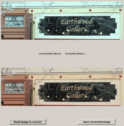 Uncorrected and corrected images |
This method works only with single images, not batches.
2. Apply the matrix in the Imatest Image Processing module
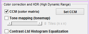 In Imatest 5.0+ the Image Processing module can be used to apply a Color Correction Matrix (saved from Color/Tone Interactive as a CSV file, as described above) to individual images or to batches of images. To do so, check the CCM (color matrix) checkbox on the left of the Image Processing window. The matrix is applied before the highly nonlinear tone mapping and bilateral filter operations.
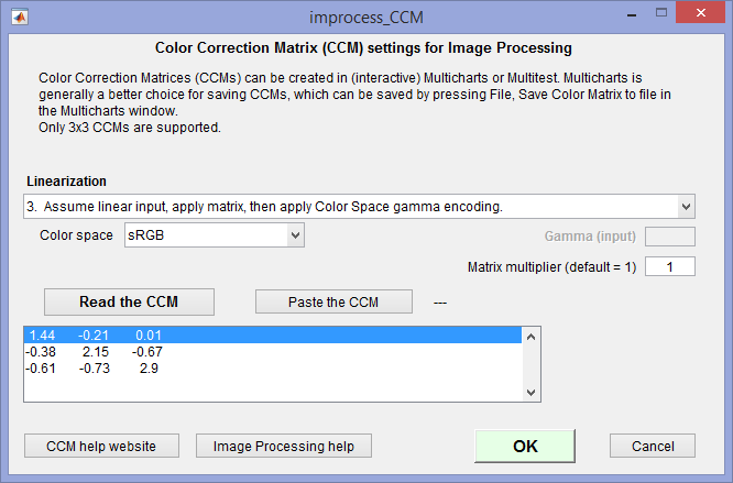
CCM settings can be entered or viewed by clicking the Set CCM button to the right of the checkbox. The key settings include linearization (described above), Color space, input gamma (for one linearization setting), and the matrix multiplier (which is can lighten or darken the image; it is normally left at 1).
CCM settings for Image Processing
Image Processing can operate on batches of images simply be selecting multiple images instead of a single image. If a batch of images has been selected, files named root_file_name.ext will be automatically saved as root_file_name–ext-improc.png.
3. Apply the matrix externally with Matlab code
Uncorrected image
The CCM can be applied outside of Imatest. We show an example, using Matlab, of how to apply the matrix. You can try this out if you have Matlab (or convert it into another language like C or Python if you don’t).
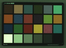
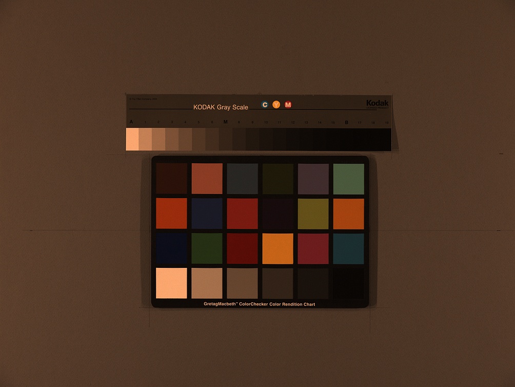
The uncorrected 24-patch Colorchecker image shown on the right is used as the input to the Color Correction Matrix calculation. It was derived from a raw image, converted to a JPEG file with no color correction, then reduced. You can click (or right-click) on it to download it.
This image was read into Color/Tone Interactive, then color-corrected with the following settings.
Optimize: Delta-E 00
Linearization: Assume linear input, apply matrix, then apply Color Space gamma encoding.
Weighting: 2. Emphasize highlights
Chroma multiplier: 1.06
Calculate XYZ matrix…
Here are the results of the correction. The corrected colors are extremely accurate— better than we usually get when we apply the matrix to an image that has already been processed (ΔEab mean = 5.32; ΔE00 mean = 3.11).
The Color Correction Matrix was obtained by clicking File, Copy color matrix to clipboard, then pasting directly into this page. You can copy it from this page if needed.
1.48663 -0.192007 0.033443
-0.612018 2.03673 -0.796356
-0.367863 -0.580001 3.04927
Corrected image
The program for applying the CCM to an image file is in the box below. It was updated July 2020 to make it much easier to run— with a simple Graphic User Interface. The core calculations, involving variable correctedRGB, can be used as a template for developing custom code.
To load the program into your system, select the text in the box, copy it to the clipboard (control-C), paste it into the Matlab (or other) editor, then save as an m-file (ccm_test.m).
Before you run ccm_test you should calculate a CCM using the Color/Tone module. If you don’t have an image of your own to test, download the uncorrected image (above) and copy the 3×3 CCM (also above) to the clipboard.
To run ccm_test from the Matlab command window.
- If possible, copy the CCM to the clipboard (using the File dropdown in the Color/Tone module or Control-C in a text file). You can select the 3×3 CCM text (above) in the browser window, then copy it (control-C).
- Enter ccm_test.
- A window with basic instructions opens. Click OK.
- A narrow window opens where you can
- enter gamma (1 for uncorrected file (above): you can derive gamma from the density plot in Color/Tone Interactive)
- enter the CCM (easiest if you paste it from the clipboard).
- A window opens that lets you browse to the image file and open it.
- The corrected image appears. You can save it if you wish.
An output image (the above input image, corrected) is shown on the right.
function ccm_test
% Test program for applying Color Correction matrix.
% Output for display gamma = 2.2 — sRGB and Adobe RGB color spaces.

uiwait(msgbox(['We recommend that you calculate the Color Correction Matrix (CCM),' newline ...
'and copy Color Matrix to the clipboard before running ccm_test.' newline newline ...
'After you click OK, two input dialog boxes will open.' newline newline ...
'1. a narrow box for entering the encoding gamma and entering or pasting the CCM.' newline ...
'2. A box for browsing and opening the image file to be corrected by the CCM.'], ...
'ccm_test instructions'));

answer = inputdlg({'Enter encoding gamma (typically 0.5-1)'; 'Paste or enter the 3×3 CCM into this box'}, ...
'Enter gamma and CCM', [1 20; 3 20]);
gamma = str2num(answer{1}); %#ok
ccmnum = str2num(answer{2}); %#ok
szcc = size(ccmnum); % Keep for diagnostics.
if isempty(answer{2}) || szcc(1)<3 || szcc(1)>4 || szcc(2)<3 || szcc(2)>4
ans2 = answer{2}; % sz2 = size(ans2),
ccmnum = [str2num(ans2(1,:)); str2num(ans2(2,:)); str2num(ans2(3,:))]
gamtemp = str2num(ans2(6,:)); %#ok
if isempty(answer{1}) && ~isempty(gamtemp)
gamma = gamtemp;
end
if isempty(ccmnum)
disp(['CCM is empty or badly-sized– try again.' newline 'szcc = ' num2str(szcc)]);
return;
end
end

[im,path] = uigetfile('*.*','Enter the image file to be corrected by the CCM'); % Find image file
imagefile = fullfile(path,im);
if im==0 | isempty(path) | isempty(im), return; end %#ok

imageRGB = imread(imagefile); % Read the image file.
imtype = class(imageRGB); % Image type: typically uint8 or uint16.
imageRGB = double(imageRGB)/double(intmax(imtype)); % Normalize to maximum for image type.
figure; image(imageRGB);
title(['Original image: gamma = ' num2str(gamma)]); % Works without Image Processing Toolbox.

linearRGB = imageRGB.^(1/gamma); % Linearize the image (apply inverse of encoding gamma).

% Change to 2D to apply matrix; then change back.
[my, mx, mc] = size(linearRGB); % rows, columns, colors (3)
linearRGB = reshape(linearRGB,my*mx,mc);
correctedRGB = linearRGB*ccmnum;
correctedRGB = min(correctedRGB,1); correctedRGB = max(correctedRGB,0); % Place limits on output.
correctedRGB = correctedRGB.^(1/2.2); % Apply gamma for sRGB, Adobe RGB color space.
% Deal with saturated pixels. Not perfect, but this is what cameras do. Related to “purple fringing”.
correctedRGB(linearRGB==1) = 1; % Don't change saturated pixels. (We don't know HOW saturated.)
correctedRGB = reshape(correctedRGB, my, mx, mc);

figure; image(correctedRGB); title('Corrected image');

tosave = questdlg('Do you want to save the corrected image?','Save the corrected image?', 'Yes','No','No');
if strcmpi(tosave,'Yes')
[path,imroot,ext] = fileparts(imagefile);
imsave = [imroot '-CCM-corr' ext];
sfile = fullfile(path,imsave);
[savef, savepath] = uiputfile(fullfile(path,'*.*'), ...
'Enter a file name to save the CCM-corrected results; empty otherwise', sfile);
savefile = fullfile(savepath,savef);
imwrite(correctedRGB, savefile);
disp(['Results written to ' savefile]);
end
Links
Some of the background for the calculation can be found in Color Correction Matrix for Digital Still and Video Imaging Systems by Stephen Wolf, though the Imatest calculation differs in many respects: there is no issue with outliers and optimization is performed using one of the standard color difference metrics.