Analysis of random scale-invariant patterns,
including the Spilled Coins (Dead Leaves) Pattern,
for measuring texture sharpness
Introduction – Scale-invariant charts – Obtaining – Photographing – Running – Automatic ROI detection
Output – MTF – MTFnn, MTFnnP – Power Spectral Density – Equations & Scale-invariance
Related pages: Texture examples – Dead Leaves measurement issue – Random/Dead Leaves cross method
Introduction
Random/Dead Leaves, which runs under the interactive Rescharts interface or as a fixed (non-interactive, batch-capable) module, measures SFR (Spatial Frequency Response) or MTF (Modulation Transfer Function) from random scale-invariant (or approximately scale-invariant) test charts, including “Dead Leaves” and “Spilled Coins” charts. It is primarily used to measure the effects of image processing, most importantly, bilateral filtering, on image texture and appearance.
Bilateral filters are a widely-used type of edge-preserving noise-reduction filter, almost universal in JPEG files from cameras, that sharpen images near edges, but smooth them in relatively flat areas, where noise is most visible. They are nonuniform, i.e., their behavior varies in different parts of the image. They cause edges to appear sharper than fine texture, and they cause slanted-edge MTF measurements to indicate better sharpness than is visible in texture. When bilateral filtering is present, spilled coins results are more representative of typical image appearance. Another Imatest chart/module that shows how sharpness varies as a function of feature contrast is Log F-Contrast.

Ceci n’est pas le mire des pièces renversées ou une pipe.
Dead leaves/Spilled Coins charts are of increasing interest because their statistics resemble those of natural scenes; they are less affected by edge sharpening than other patterns (especially the slanted-edge), and hence provide estimates of texture detail that correlate better with perceptual observations. They are the basis of a proposed ISO standard for Texture blur measurements (from Technical committee ISO TC 42/WG 18).
The Imatest Spilled Coins chart (released January 2013) has several advantages over existing Dead Leaves charts. Most importantly it is almost perfectly scale-invariant, and hence produces more reliable and consistent results. Scale-invariant means that the pattern statistics (especially frequency spectrum and contrast) are independent of magnification, i.e., do not vary with camera-to-target distance, cropping, or pixel dimensions. This greatly simplifies setup and analysis— advantages are described here. This requirement is met by random (or nearly random) patterns that have a 1/f frequency spectrum (a 1/f 2 Power Spectral Density (PSD) ).
Spilled Coins charts can be purchased from the Imatest Store.
Scale-invariant test charts
Random/Dead Leaves supports two types of scale-invariant chart: Dead Leaves or Spilled Coins charts, which consist of stacked randomly-sized circles (resembling spilled coins far more than dead leaves), and purely random charts.
The advantages of scale-invariant charts are described below.
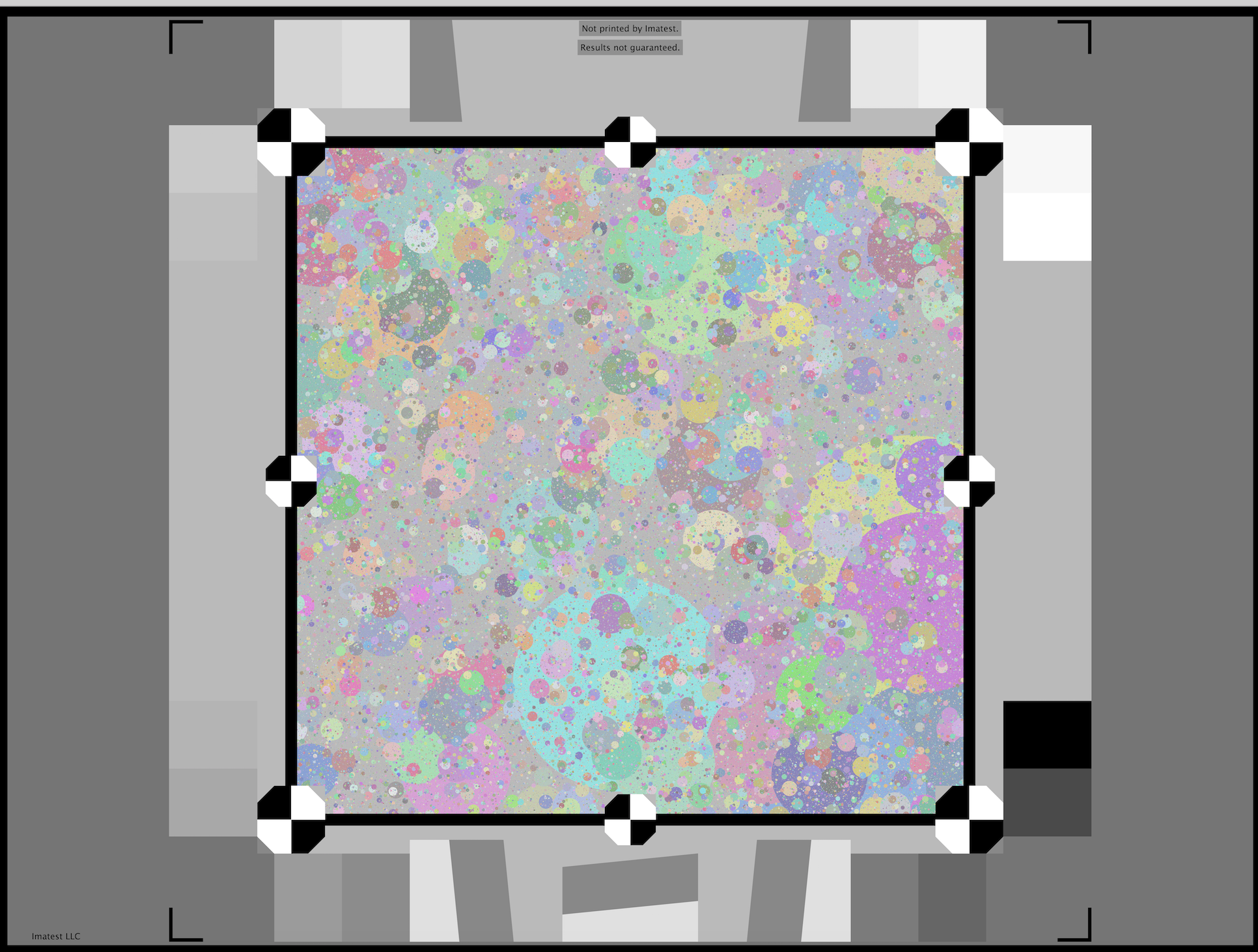
The Imatest Spilled Coins (Dead Leaves) chart
 chart")
The Imatest Spilled Coins chart (a variant of the Dead Leaves chart with nearly perfect scale-invariance)
has several advantages over other Dead Leaves charts.
Key features of the Spilled coins chart:
-
The Spilled Coins (dead leaves) pattern in the central region is almost perfectly scale-invariant (unlike conventional dead leaves charts), allowing it to be used for reliable MTF measurements that correlate well with other methods for RAW images (which do not have nonuniform or nonlinear processing).
 chart")
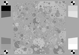
The color Spilled Coins chart has the same scale-invariant (1/f) frequency spectrum as the monochrome chart, but may respond slightly differently to noise-reduction signal processing.
- Maximum contrast range is 3:1, as called for in the CPIQ Phase 3 draft Texture Blur Metric draft specification..
- A color version (central area shown on the right) is available.
- It is more uniform, i.e., is more shift-invariant than other Dead Leaves charts.
- It contains slanted edges (2:1 and 4:1 contrast) for convenient comparisons with the Spilled Coins pattern.
- Noise compensation: The gray area to the left and right of the Spilled Coins pattern has the same mean density as the pattern itself. The noise Power Spectral Density (PSD) calculated from these regions can be subtracted from the signal+noise PSD in the central Spilled Coins region to obtain the PSD of the pattern itself, with noise removed. This technique is described in Equation (6) of “Texture-based measurement of spatial frequency response using the dead leaves target: extensions, and application to real camera systems” by Jon McElvain, Scott P. Campbell, Jonathan Miller, and Elaine W. Jin, presented at Electronic Imaging 2010.
- Registration marks and 16 grayscale patches are included. The linear levels used to create the grayscale patches are 0 through 255 in steps of 17 (same as the Siemens Star chart in the draft of the upcoming ISO 12233 standard). The black outline makes it easy to align the chart.
| Spilled Coins chart sizes | Spilled Coins region | Printed region | Media size total |
| Large | 12×12 in (305x305mm) | 22.4×16.8 in (569x426mm) | 24×18 in (610x458mm) |
| Medium | 8×8 in (203x203mm) | 14.93×11.2 in (379×284 mm) | 16×12 in (458x305mm) |
| Small | 6×6 in (152x152mm) | 11.2×8.4 in (284x213mm) | 12×10 in (305x254mm) |
| LVT (film) | 5.536×5.536 in (141x141mm) | 9.25×7.75 in (159x197mm) | 10×8 in (254x203mm) |
| Dead Leaves charts are designed to catch problems like this one: a crop of an image from an early 8 megapixel camera phone that had sharp edges (from strong software sharpening; the lens wasn’t great), but had severe texture loss (in the pines; from software noise reduction designed to reduce noise from the tiny pixels). Click here to view a crop of a spilled coins image from this camera and a detailed analysis.Image like this remind me of the classic Ghostbusters line: “He slimed me.“ |  |
The Random Scale-Invariant chart
 Random scale-invariant test chart, with random pattern in center
The Random Scale-Invariant chart, which can be printed from the Imatest Test Charts module, has the same structure as the Spilled Coins chart. The random scale-invariant pattern in the center occupies the majority of the real estate.
Algorithm: The chart starts out as a uniformly distributed random pattern with values between 0 and 1. It is then Fourier transformed into 2D frequency domain, the magnitude of the FFT is forced to have a 1/f frequency spectrum, then it is Fourier transformed back to spatial domain.
The two smooth regions on the left are used to measure that noise Power Spectral Density (PSD) that can be used to remove the noise power of the central random pattern using the McElvain-Campbell-Miller-Jin. technique, referenced above.
Differences between the charts
Although both charts have similar frequency domain characteristics (1/f Fourier transform = 1/f 2 Power Spectral Density), they are markedly different in the spatial domain. The Random pattern lacks any edges or sharp features while the Spilled Coins (dead leaves) pattern has a moderate number of edges, most with relatively low contrast (below the maximum contrast ratio of 3:1).
The Random pattern is the extreme pattern for noise reduction: it maximizes it while minimizing sharpening. The Spilled Coins pattern is more representative of real images: it has a few edges and quite a significant amount of fine texture. It has achieved traction if the imaging industry, especially with the Camera Phone Image Quality (CPIQ) group.
Obtaining and photographing the chart
The Spilled Coins chart is available from the Imatest store. The Random chart is also available.
|
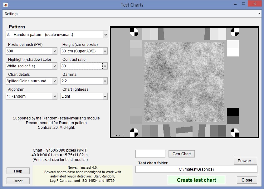
A TIFF file for printing a Random Scale-Invariant test chart can be created using Imatest Test Charts. Typical settings are shown below. Warning: Do not attempt to print a chart unless you have a high quality photographic printer and
In the standard Random Scale-Invariant chart, shown above, the scale-invariant random pattern occupies the middle 75% of the image. The right side contains a 16-patch grayscale step chart, with densities in increments of 0.1, and a low contrast (2:1) slanted edge whose average density equals that of the random pattern. The slanted edge can be run with SFR for comparison. The left side contains two patches for measuring noise (for subtracting noise Power Spectral Density from the random pattern PSD). |
Mount the chart on a flat medium gray to black board— 1/2 inch (12.5mm) foam board works well; thinner board warps more easily. We recommend using a spray adhesive (such as 3MTM Super 77 or Photo Mount) or double-sided tape (such as 3MTM #568 Positionable Mounting Adhesive). Depending on the number of horizontal pixels in the chart to be analyzed, the chart should occupy 1/3 to 1/4 of the horizontal frame. Other charts can be mounted along with it.
Orientation. The pattern should be oriented horizontally, i.e., in landscape orientation (it is slightly wider than high).
Photograph the chart using the sort of lighting described in Imatest Lab or How to test lenses, taking care to avoid glare. Save the image in any one of several high quality formats, but beware of JPEGs with high compression (low quality), which will show degraded quality, unless, of course, you are testing for JPEG degradations.
|
Because resolution varies over the image for most cameras and lenses, the chart should not take up too much of the frame.
This recommendation does not apply to low resolution systems such as VGA, which need at least 300 pixels of active chart height (more if possible). |
Running the program
Running interactively in Rescharts
Open Imatest, then click . The Rescharts window is described in the Rescharts page. Click on the Chart Configuration dropdown and choose the appropriate setting for the chart to be analyzed.
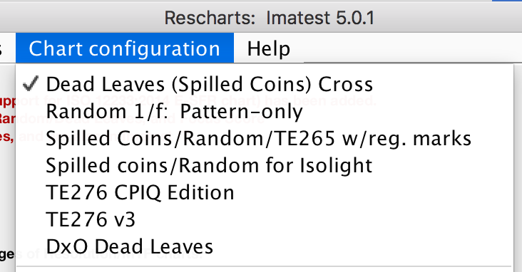
| Dead Leaves (Spilled Coins) Cross | Imatest’s color spilled coins chart with 8 registration-marks around the pattern. |
| Random 1/f: Pattern-only | No grayscale or gray patches. |
| Spilled Coins/Random/TE265 w/reg. Marks |
Imatest Spilled Coins or Random chart with grayscale patches on the sides and registration marks near corners (also the Image Engineering TE265 Dead Leaves chart). Automatic region detection is available. |
| Spilled coins/Random for Isolight |
Imatest Spilled Coins or Random chart with more tightly-located registration marks (and fewer grayscale patches) for use with the Isolight. |
| TE276 CPIQ Edition | v2 of the Image Engineering TE276 chart, with large noise-PSD patch on the side |
| TE276 v3 |
v3 of the Image Engineering TE276 chart |
| DxO Dead Leaves | DxO’s original Dead Leaves chart design |
| Select a pattern to analyze (in this case, Random / Dead leaves) by clicking on the appropriate entry in the popup menu below or by clicking on if Random… is displayed. The button and popup menu (shown on the right) are highlighted (yellow background) when Rescharts starts.
Select the image to read. If the pixel size is the same as the previous Random run, you’ll be asked if you want to use the previous ROI, adjust the previous ROI, or crop anew. If the folder contains meaningless camera-generated file names such as IMG_3734.jpg, IMG_3735.jpg, etc., you can change them to meaningful names that include focal length, aperture, etc., with the View/Rename Files utility, which takes advantage of EXIF data stored in each file. |
 |
Running as a fixed (batch-capable) module
Random/Dead Leaves can also be run as a fixed module, capable of analyzing batches of files. Click (in the Imatest main window) or Fixed Modules, Random. Select a file or group of files. If the image is the same size as a recently-run image (several sizes are saved) you’ll be asked if you want to repeat the same regions of interest.
Cropping
For standard Random or Spilled Coins images, make the initial crop on the outside of the registration marks. Your initial ROI selection doesn’t have to be precise because it can be refined in the ROI fine adjustment window, shown below. The ROI fine adjustment window may be maximized to facilitate fine selection.
 chart") ROI fine adjustment window for a Spilled Coins (or Dead Leaves) image
ROI fine adjustment window for a Spilled Coins (or Dead Leaves) image
| Automatic region detection is available for Imatest Spilled Coins/TE265 Dead Leaves charts starting with Imatest 4.0.Automatic/manual region detection must be selected before running Random, by pressing in the Imatest main window. The relevant portion is shown below.
Of the three Random dropdown menu selections, the first is the traditional manual ROI selection method. The second is for automatic detection with the Fine Adjustment window shown after auto selection for confirmation (and adjustment, if needed). The third is for fully automatic detection without confirmation. Alternatively, Automatic/manual region detection can also be selected (for the next run) in the settings window, as described below. There are two dropdown menus to the right of Automatic ROI selection. The first has three selections related to automatic detection: The second has two settings related to the settings window that can appear after the region selection. |

If you press (Express mode is not selected), the settings window shown below appears. This window can be at any time by pressing the button.
Settings
Title defaults to the file name. You can enter a description of the system if needed.
Settings area
Chart configuration (Dead leaves (Spilled Coins or TE265) shown) duplicates the Region selection dropdown menu in the Rescharts window. It indicates how to handle the graphics that surround the main pattern. Affects the next run. (Added for the fixed version of Random.)
Region selection for next run (manual or automatic) lets you select manual or automatic region selection (with or without ROI confirmation). Added in Imatest 4.0.
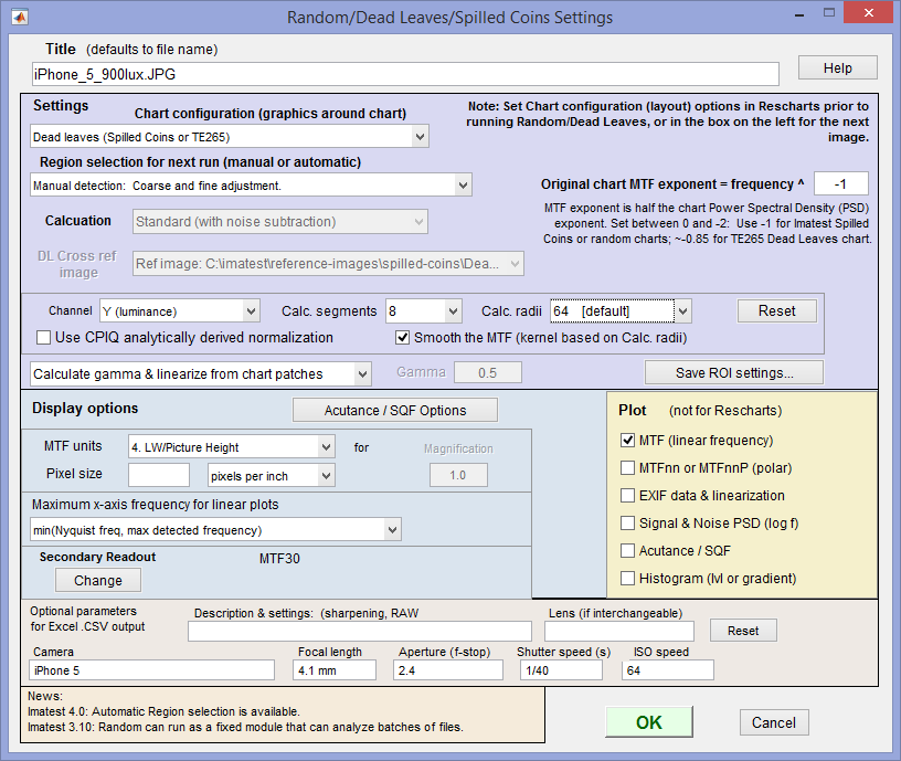 Random/Dead Leaves settings window
| Original chart MTF exponent is the critical setting for obtaining correct MTF measurements.For the Spilled Coins and Scale-Invariant Random charts, set the exponent to -1. (This is the value for scale-invariance.) For the TE265 Dead Leaves chart, set the exponent to -0.85 ±0.02. This number is approximate. If you have the original chart file or a very high quality image of the chart that fills the frame (obtained with a high quality lens at optimum aperture, taking special care that the image is in focus— important because some autofocus systems don’t focus well on Dead Leaves or random patterns), you can determine the exponent. See PSD (below) for details. |
Channel is R, G, B, or Y (luminance; the default). The Luminance (Y) channel, which corresponds to human perception, is defined as Y = 0.2126*R + 0.7152*G + 0.0722*B. The Options III window lets you select between this recommended value and an older (NTSC-based) value of 0.3*R + 059*G + 0.11*B.
Calc segments is the number of segments in 2D frequency domain to analyze. 8, 12, and 24 are supported. 8 is the default, but 1 is usually sufficient. Derived from Star chart, where segments are calculated in the spatial domain, which may be more meaningful. may be dropped in the future.
Calc segments is the number of angular segments in 2D frequency domain to analyze. 8, 12, and 24 are supported. 8 is the default, but 1 is usually sufficient. A maximum of 8 angular segments can be displayed in regular MTF plots, but all segments are shown in angular (MTFnn, MTFnnP) plots.
Calc. radii is the number of radii on the circle used for the MTF calculations. 64 is sufficient in most cases. 32 is faster and less susceptible to noise; 128 has a finer frequency gradient, but is more susceptible to noise and slower (not recommended).
Enter or calculate gamma Choose between Calculate gamma & linearize from chart patches or Enter gamma for linearization. If Calculate gamma… is selected, the 16 patch step chart to the right of the random pattern is used to determine the value of gamma for linearizing the chart, Gamma (below) is disabled, and the displayed value of gamma includes the indicator (chart).
Gamma is used to linearize the test chart when Enter gamma… (above) is selected. It can be measured by Stepchart, Colorcheck, or Multicharts. 0.5 is a typical value for color spaces intended for display at gamma = 2 2 (sRGB, Adobe RGB, etc.). If gamma is entered (rather than calculated), the displayed value of gamma includes the indicator (input).
Save ROI settings… lets you save ROI settings using the method described in How to store and retrieve region selections.
Display area
MTF plots selects the x-axis scaling. If Cycles/inch, Cycles/mm, or any of the Cycles/angle settings are selected, the pixel spacing (um/pixel, pixels/inch, or pixels/mm) should be entered.
X-axis scaling for linear plots selects the maximum spatial frequency to be displayed in linear plots.
Secondary readout allows up to two secondary redouts (MTFnn, MTFnnP, or MTF at a specified spatial frequency) to be displayed on the MTF plots. Details here.
Don’t worry about getting all settings correct: You can always open this dialog box by clicking on in the Rescharts window.
After you press , calculations are performed and the most recently-selected display appears.
Random-Cross method:
 The Random- or Dead Leaves-Cross Correlation method is an alternative texture analysis method. The main difference with the Power Spectral Density-based method (often called the “Direct” texture method in the literature) is that the Cross method is uses a reference image file to perform cross-correlation between the true and observed texture patterns. This graduates the method from relying on statistical information about the pattern to relying on the pattern itself (going from a semi-reference metric to a full-reference metric), which lends allows for stronger assumptions about the results.
Further information is available on the Random-Cross texture analysis page.
Plot (not for Rescharts)
The five plots in this section are available as output figures. They are referenced as Plot n in fixed module in the table, below. EXIF data appears on the right side of Plots 1 and 4.
Output
The Display box in the Rescharts window, shown below, allows you to select any of several displays. Display options are set in boxes that appear below Display. All displays except Exif data have a channel selection option (Red, Green, Blue, or Luminance (Y) (0.3R + 0.59G + 0.11B).
| Display | Description |
| 1. MTF (linear frequency) Plot 1 in fixed module |
MTF for up to 8 segments (in frequency domain). Linear frequency display. |
| 2. MTF (log frequency) | MTF for up to 8 segments. Logarithmic frequency display. |
| 3. MTFnn or MTFnnP Plot 2 in fixed module (polar) |
Display MTF contours (MTF70 through MTF10, if available) in a polar or rectangular plot. Only meaningful if >1 Calc. segments selected. |
| 4. EXIF data and linearization Plot 3 in fixed module |
Show EXIF data if available as well as linearization curves (used to calculate gamma from the chart). |
| 5. Signal & Noise PSD (linear f) | Show Signal + Noise, Noise, and Signal (noise removed) Power Spectral Density with a linear frequency display. |
| 6. Signal & Noise PSD (logarithmic f) Plot 4 in fixed module |
Show Signal + Noise, Noise, and Signal (noise removed) Power Spectral Density with a logarithmic frequency display (generally more useful). |
| 7. SQF/Acutance Plot 5 in fixed module |
Display Subjective Quality Factor or CPIQ Acutance. The CPIQ JND (Just Noticeable Difference) can also be plotted. |
| 8. Display image | Display the image with any of several options (cropping, lighten, color boost, etc.). |
| In addition to the displays, two buttons allow you to save results. | |
| Saves an image of the Starchart window as a PNG file. If you check Display screen in the Save screen dialog box, the image will be opened in the editor/viewer of your choice. (Irfanview works well, and it’s free.) | |
| Saves detailed results in a CSV file that can be opened by Excel and also in an XML file. | |
The spatial frequency is automatically calculated from the image, under the assumption that log frequency increases linearly with distance. The number of chart cycles is also determined automatically.
MTF
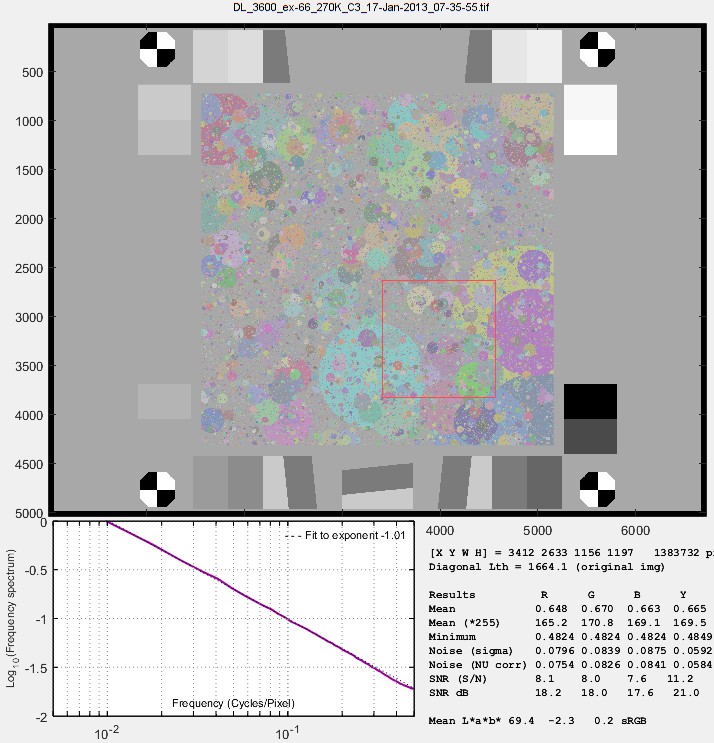
The results shown below are for the Panasonic Lumix DMC-G3 (Micro Four-Thirds) camera with a 14-45mm f/3.5-f/5.6 zoom lens, set at ISO 800, f/8, 28mm. Both raw and JPEG images were saved. Raw results will be displayed first; JPEG results for the same image will be shown later for comparison. Crops of the images used to obtain these results are on Texture examples.
The MTF (Spatial Frequency Response, normalized to 1.0 at low spatial frequencies*) can be displayed on a linear or logarithmic frequency scale. The mean response for the 8 (directional) segments is displayed as a thick magenta-gray curve.
*MTF is normalized to the highest value of the second or third MTF array element. The first value is not used because the original chart MTF is not reliably scale-invariant at that frequency and because it it is highly sensitive to uneven illumination.

MTF (linear frequency scale) for 8 segments of the Spilled Coins pattern (Plot 1 in fixed module)
(raw image; default demosaicing). Click here to view a crop of the raw image.
Gamma = 0.526 (chart) at the lower left of the plot indicates that gamma was calculated from the 16 grayscale patches near the corners of the Spilled Coins pattern. Gamma can also be entered directly as an input value.
 MTF50, MTF50P, MTF20, MTF20P, MTF10, and MTF10P for the first 8 angular segments are displayed in a table just below the plot. Measurements are omitted where MTF doesn’t drop below the specified level. The pale dashed line, which settles around 0.35 between 0.35 and 0.5 (Nyquist) Cycles/Pixel, is the MTF without noise reduction. The mean MTF above 0.4 C/P is affected very little by the choice of dcraw demosaicing algorithm, but the differences between the segments is strongly affected (they’re much lower when demosaicing quality is set to -q 2: Patterned pixel grouping— shown on the right). We obtained similar results with Silkypix SE, the raw converter supplied with Panasonic cameras.
Because the raw image (straight out of the sensor) has been converted using dcraw, which applies no spatial image processing (sharpening or noise reduction), we expect the MTF to be close to the MTF derived from a slanted-edge. We can compare them, by selecting 1. Slanted-edge SFR from the dropdown menu just below . The noise reduction box should be checked; the curve is much bumpier if it’s unchecked.

MTF from a 4:1 contrast slanted-edge from the same raw image.
The Spilled Coins and slanted-edge MTFs track closely up to 0.4 cycles/pixel. Above 0.4 C/P MTF is higher from Spilled Coins.
| We have found that discrepancies between Spilled Coins and slanted-edge MTF measurements are primarily caused by demosaicing, which is a type of nonlinear processing that handles edges and random noise quite differently. Details are shown on the Texture examples page. As a result, the Power Spectral Density (PSD) subtraction algorithm works imperfectly. There results were consistent at ISO 160 and ISO 800. |
Power spectral density (PSD)
|
6. Signal & Noise PSD (logarithmic f) in the Display dropdown menu displays the PSD with a logarithmic frequency scale (more useful than a linear scale because PSD response is exponential). This is the PSD of an original image used to create the Spilled Coins chart.
The slope of the dashed red line is the Chart MTF exponent, entered in the Settings window, described above. You can do repeated runs with different values of this exponent until you get a good match for the appropriate frequency range. |
 Original chart. Click here to view a crop of the image. Original chart. Click here to view a crop of the image.Plot 4 in fixed module |
| Next we show the PSD of the raw image. The plot on the right shows the original signal+noise PSD from the Spilled Coins area (bold red line), the noise PSD from the gray areas to the left and right (bold brown line), and the signal PSD of the Spilled Coins area after the noise PSD has been subtracted (bold blue line) using the McElvain et. al. technique. Spatial frequency is displayed on a logarithmic scale.This plot is primarily a check to verify that an appropriate amount of noise has been subtracted from the S+N signal so that a correct value of MTF is calculated and displayed (i.e., so that noise does not masquerade as signal— valid MTF response).
Plot 4 in fixed module |
 PSD and noise of the raw image PSD and noise of the raw image |
MTFnn, MTFnnP of the raw image
|
 MTF70-MTF10 polar display MTF70-MTF10 polar display(spatial frequency in C/P displayed radially) |
Raw-JPEG comparison
Unlike RAW images, JPEG camera output has been processed. Sharpening is almost always applied (with good reason: it always improves perceptual image quality unless it’s overdone). Noise reduction is frequently applied (though less consistently than sharpening), particularly at high ISO speeds where noise may be objectionable.
MTF— Spilled Coins pattern (JPEG)
|
 MTF for 8 segments of the Spilled Coins pattern MTF for 8 segments of the Spilled Coins pattern(JPEG image). Click here to view a crop of the image. |
MTF— Slanted-edge (JPEG)
|
 MTF from a 4:1 contrast slanted-edge MTF from a 4:1 contrast slanted-edgefrom the same JPEG image |
Power Spectral Density and noise (JPEG)
|
 PSD and noise of the JPEG image PSD and noise of the JPEG image |


| The details of the pattern differ, but the overall statistics change very little.A problem with non-scale-invariant patterns is that image sensor/camera noise does not change with magnification. Image sensor noise is, in a sense, scale-invariant. When the image is not scale-invariant, but the sensor noise is, the issue of how to subtract noise Power Spectral Density so MTF can be accurately calculated becomes rather murky.This is not a problem with scale-invariant patterns. Calculations are accurate and results are trustworthy.The most popular patterns used to measure resolution— the slanted-edge and the Siemens star— are scale-invariant, and have a 1/f frequency response with respect to the axis used to calculate spatial frequency. Scale invariance makes MTF measurements very convenient for these patterns, and is a large part of the reason for their popularity. |  1/16 X 1/16 X |
|
| Scale-invariance function For a function f(x) with Fourier transform (F(ω)), the scaling property of Fourier transforms states that
f(ax) → F(ω/a) ⁄ |a| A function is scale-invariant if F(f(ax)) = F(f(x)) . Although it is difficult to derive a general solution for F, we can look at the case where F(ω) = 1/ω and a > 0. F(f(ax)) = F(ω/a) ⁄ |a| = (a/ω) ⁄ a = 1/ω = F(f(x)). Hence we can say that charts with F(ω) = 1/ω are scale-invariant. Since Power spectral density PSD is proportional to the square of the MTF, PSD(ω) ∝ 1/ω2 for scale-invariant functions. The exponents of MTF and PSD are -1 and -2, respectively.
Imatest Image Statistics display showing MTF curve
Dead Leaves chart crop The Spilled Coins chart is created in different order from Dead Leaves charts. Instead of laying down circles in random order, they are laid down sequentially— largest to smallest, using a different distribution of circle sizes. This makes the Spilled Coins chart much more scale-invariant. With the Dead Leaves chart, large circles added near the end of the process have an adverse effect on both the spectrum and shift-invariance, which can be conveniently examined with the Image Statistics module by selecting square or rectangular areas at various positions around the image. It’s easy to see that the Imatest Spilled Coins chart is very shift-invariant, especially compared to other charts. |
||

References
 Dead Leaves Can Dance |