Introduction – Test chart – Photograph the chart – Framing – Lighting
Distance – Exposure – Run Imatest – Select files – Settings – Warnings – clipping
Batchview (combined results) – Checklist
Testing lenses: Introduction
Lens quality (especially sharpness) has always been of major interest to photographers. Traditionally, lens testing has been highly tedious, best left to professionals and large publications. With Imatest, that has changed forever. All you need to do is photograph an SFRplus, eSFR ISO, or tilted Checkerboard chart (with careful technique of course), run the corresponding module (SFRplus, eSFR ISO, or Checkerboard), and interpret the results.
The three modules described here all uses slanted-edges with automatic Region of Interest (ROI) detection. Slanted-edges are particularly valuable for lens testing because they use space efficiently, and hence can map sharpness over the image surface. Different slanted-edge charts and modules are compared here.
Imatest measures the sharpness of the entire imaging system— the lens, sensor, and image processing (especially sharpening)— not just the lens. This may sound complicated, but when several lenses are tested on the same camera with the same settings, they may be fairly compared.
Key image quality factors
- Sharpness, (the most important) which is characterized by spatial frequency response (also called MTF for Modulation Transfer Function). Although the complete MTF response curve is of interest, the spatial frequencies where contrast falls to half its low frequency and peak values, MTF50 and MTF50P, are simple and useful indicators of both image and lens sharpness. Their relationship to print quality is discussed in Interpretation of MTF50 and SQF/Acutance.
- Lateral chromatic aberration, which can appear as color fringing near the edges of the frame,
- Distortion (barrel or pincushion; SFRplus and Colorcheck have the most detail),
- Tonal response, gamma, and color response (not in Checkerboard).
Imatest’s full set of image quality factors is described here.
Imatest SFRplus and eSFR ISO are straightforward to use and produce clear numeric results, but careful technique is vital.
To fully characterize a lens you should test it with a variety of settings.
- Aperture: most lenses are relatively soft wide open and sharpest around the middle of their range (the “optimum” aperture): around f/5.6 to f/11 for the 35mm and digital SLRs; f/2.8-f/5.6 for compact digital cameras. Included in the EXIF data.
- Focal length in zoom lenses also strongly affects sharpness, but there is no general trend relating sharpness to focal length. Included in the EXIF data. Three focal lengths are usually sufficient for ordinary zooms (with a zoom, i.e., focal length ratio under 5:1). Five are recommended for extreme (super) zooms.
- Locations on the image plane: Lenses tend to be softer toward the edges. For this reason you should test sharpness at several locations in the frame (easy with the modules described here). We recommend at least 13 regions (more are better) to fully characterize a lens: 1 near the center, 4 part-way out (near the top, bottom, and sides), 4 near the corners, and top, bottom, left, and right. More regions can give a more detailed characterization, especially with 3D and lens-style MTF plots. In a well-manufactured lens, sharpness should be symmetrical about the center of the image, but we live in an era when manufacturers are constantly striving to reduce production costs, often at the expense of manufacturing quality. Even premium lenses may be poorly centered. Decentering is particularly well displayed in the 3D plots.
You can learn a lot by testing your own lenses, but you must be aware of two essential facts.
You cannot measure a lens in isolation. It is a part of an imaging system that includes the camera’s image sensor, RAW converter (which may sharpen the image), and image processing pipeline. Hence,
Lenses vary from sample to sample. Measurements may differ. |
The basic steps in testing the lens are:
- Purchase or print an SFRplus or eSFR ISO test chart and mount it on a flat surface.
- Photograph it in an environment with even, glare-free lighting.
- Use the Rename Files module to rename the files to more meaningful names, based on EXIF data contained in the file. For example, the name can include a brief description, the ISO speed, the aperture, etc. Make sure you have the correct EXIF setting (Get … EXIF data from Phil Harvey’s Exiftool) in the Options II window.
- Run Imatest. Imatest Instructions– Getting started (updated in 2021) is strongly recommended.
- Run Imatest SFRplus Setup or eSFR ISO Setup (Interactive mode) or SFR plus Auto (or eSFR Auto; for batches of files.
- Interpret the results.
The test chart
The SFRplus chart was designed to measure a large number of key image quality factors, including sharpness, lateral chromatic aberration, and distortion. More about the chart can be found in Using Imatest SFRplus, Part 1. Here is a standard monochrome SFRplus chart, which is available in several options, listed in the table below.
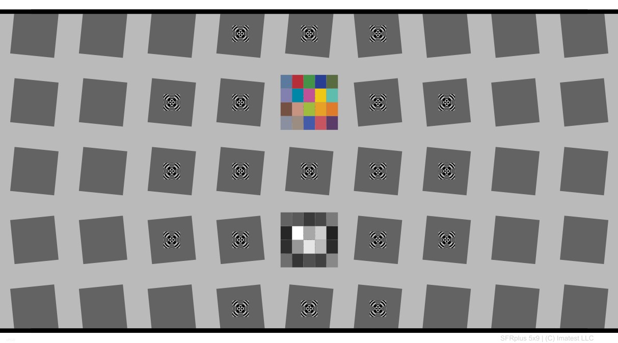 Standard SFRplus test chart
| Standard | Options & notes | |
|---|---|---|
| Grid of squares | 5×9 | 4×7, 5×7, and 7×11 are also available. 5×9 is best suited for HTDV (16:9 aspect ratio) and DSLRs (3:2 aspect ratio). 5×7 is best suited for compact digital cameras and cameraphones (4:3 aspect ratio). |
| Main contrast level | 10:1 | from 40:1 to 1.1:1, Greater than 10:1 not recommended. |
| Secondary contrast level | 2:1 | Same as main level or as low as 1.1:1. Shows effects of nonlinear processing. |
| Stepchart | Included (below center) | Omitted in chrome on opal or glass charts |
| Color chart | not-included in self-printed charts | Included (above center). L*a*b* values can be sent in a file. |
| Focus star | (no longer standard) | Focus aids are now included in the centers of squares |
| Size | No standard size | 40 or 60 inches (1 or 1.5 meters) wide inkjet-printed, Different sizes are available on other media. |
The standard SFRplus test chart consists of a 5×7 or 5x9 grid of squares with 4:1 contrast ratio. (Older versions had 10:1 contrast ratios in most squares and 2:1 in a few selected squares.) A small 4x5 patch grayscale stepchart (densities in steps of 0.1 from 0.05 to 1.95) is located below the central square and an optional color pattern is located above the center.
The chart can be purchased from the Imatest store. It should be mounted on 32x40 or 40 x60 inch (0.8×1 or 1×1.5 meter) sheets of 1/2 inch (12.5 mm) thick foam board with spray adhesive or double-sided tape (a somewhat nerve-wracking process— consider using a local print or framing shop). 1/2 inch foam board stays flatter than standard 1/4 or 3/8 inch board.
Other media are available: chrome-on-glass transmission targets in very small sizes Details here. 8×10 inch color film, 12×20 inch B&W file, or photographic paper (finer than inkjet). Charts can be printed widebody inkjet printers, but you must have fine materials, skill, and a knowledge of color management. We strongly recommend that you purchase a chart.
|
Nonlinear signal processing (bilateral filtering) and chart contrast Although Imatest SFR is relatively insensitive to chart contrast (MTF is normalized to 100% at low spatial frequencies), measured SFR is often affected by chart contrast due to nonlinear signal processing in cameras, i.e., processing that depends on the contents of neighboring pixels, and hence may vary throughout an image. Bilateral filtering is almost universal in consumer digital cameras (though you can avoid it by using RAW images with dcraw). It improves pictorial quality but complicates measurements. It takes two primary forms.
The signal processing algorithms are proprietary; they are a part of a manufacturer’s “secret sauce”
Nonlinearities are analyzed in depth in the Log F-Contrast module. They can be simulated with the Image Processing module. |
The eSFR ISO chart (based on ISO 12233:2014/2017), which comes in Enhanced (3:2 aspect ratio) and Extended (16:9 aspect ratio) versions, was designed to measure the same image quality factors as SFRplus. More about the chart can be found in Using Imatest eSFR ISO, Part 1. Here is the Enhanced chart:
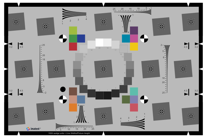 Enhanced ISO 12233 E-SFR chart, supported by the Imatest eSFR ISO module.
Photograph the chart
Framing
Frame the SFRplus chart as specified below (and in more detail in Using SFRplus Part 1). Framing for the eSFR ISO chart is described here.
- There is white space above and below the bars (used to measure distortion) at the top and bottom of the images. The white areas should be at least 0.5% and no more than 25% of the total image height. Ideally the white space should be 1-6% of the image height. The chart should be vertically centered, but this is not necessary for SFRplus to run successfully.
- The stepchart pattern is close to the horizontal center of the chart.
- The sides of the chart may extend beyond the image (as shown below) or be well within the image. The software is designed to accommodate a wide variety of framing and aspect ratios. Edges closest to the left and right boundaries will always be properly located. If the left and right sides of the chart are inside the image, there should be no interfering patterns in the image that could be mistaken for chart features— chart surroundings included within the image should be or light gray.
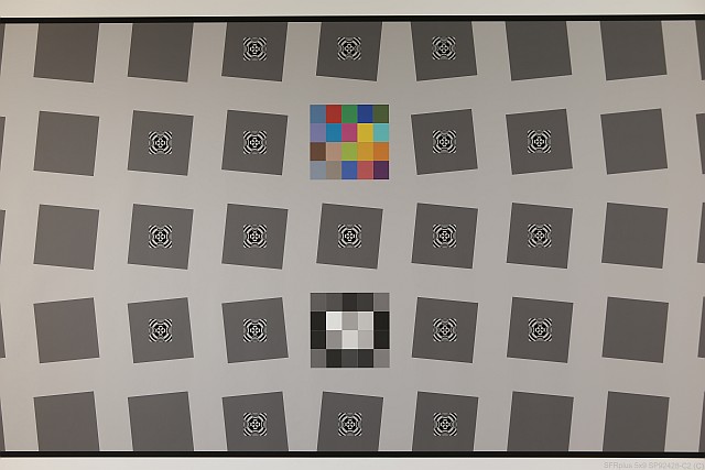
Example of a well-framed and well-exposed SFRplus image. Note that it’s OK for squares to run off the sides
- The chart should be aligned correctly using techniques and tricks shown in The Imatest Test Lab. Moderate misalignment is tolerated by SFRplus: a tilt of 1-2 degrees, perspective distortion, etc., but every effort should be made to align the chart properly. Moderate barrel or pincushion distortion (
- The image can be cropped (starting with) to remove interfering features near the edges, using the button in the SFRplus setup window.
If exposure compensation is available, you may want to use it to get a good exposure: typically by overexposing +1 f-stop.
|
Bad framing
Interfering patterns near borders (Can be cropped in Imatest 3.4+) |
Good framing
Same pattern; interfering patterns masked out |
Missing white space above top distortion bar |
Some tilt, distortion tolerated |
Lighting
The chart below summarizes lighting considerations. The goal is even, glare-free illumination. Lighting angles between 30 and 45 degrees are ideal in most cases. At least two lights (one on each side) is recommended; four or six is better. Avoid lighting behind the camera, which can cause glare. Check for glare and lighting uniformity before you expose. A description of recommended lighting setups can be found in Building a Low-Cost Test Lab. (We formerly recommended 4700K (near-daylight) SoLux quartz-halogen lamps, but we now recommend LED lamps, which are available with adjustable intensity and color temperature.) The BK Precision 615 Light meter (Lux meter) is an outstanding low-cost instrument (about $100 USD) for measuring the intensity and uniformity of illumination.

Distance
|
Choose a camera-to-target distance that gives at least the recommended image field width. The actual distance depends on the sensor pixel count and the focal length of the lens.
Exposure
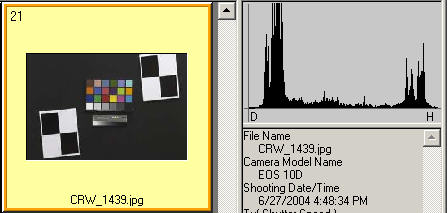
Proper exposure is important for accurate Imatest SFR results. Neither the black nor the white regions of the chart should clip— have substantial areas that reach pixel levels 0 or 255. The best way to ensure proper exposure is to use the histogram in your digital camera. Blacks (the peaks on the left) should be above the minimum and whites (the peaks on the right) should be below the maximum.
The histogram, taken from the Canon File Viewer Utility, indicates excellent exposure.
Save the image as a RAW file or maximum quality JPEG. If you are using a RAW converter, convert to JPEG (maximum quality), TIFF, or PNG. If you are using film, develop and scan it.
If the folder contains meaningless camera-generated file names such as IMG_3734.jpg, IMG_3735.jpg, etc., you can change them to meaningful names that include focal length, aperture, etc., with the Rename Files utility, which takes advantage of EXIF data stored in each file.
Run Imatest SFRplus, eSFR ISO
If you are new at Imatest, we strongly recommend Imatest Instructions – Getting started. The instructions below are excerpted from Using Rescharts Slanted-edge modules Part 2.
Open Imatest by double-clicking the Imatest icon on
- the Desktop,
- the Windows Start menu,
- the Imatest folder (typically C:\Program files\Imatest in English language installations).
After several seconds, the Imatest main window opens. Then click on , , or on the upper left.
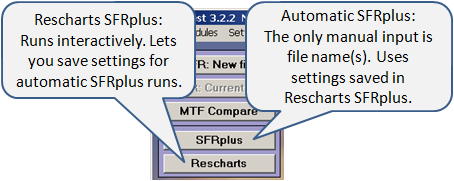
SFRplus and eSFR ISO operate in two modes: interactive/setup (Rescharts) and automatic.
Use or to initiate an interactive/setup run. This allows you to examine detailed results interactively and to save settings for the highly automated or runs (or the even more automated EXE or DLL versions included in Imatest IT). SFRplus or eSFR ISO should be run at least once in Rescharts prior to the first Auto run.
Selecting file(s)
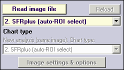
The portion of the Rescharts window used for opening files is shown on the right. You can open a file by clicking on if the correct chart type is displayed, or by selecting a Chart type. One or more files may be selected, as shown below. If you select multiple files, they will be combined (averaged), and you’ll be given the option of saving the combined file.
If the folder contains meaningless camera-generated file names such as IMG_3734.jpg, IMG_3735.jpg, etc., you can change them to meaningful names that include focal length, aperture, etc., with the Rename Files utility, which takes advantage of EXIF data stored in each file.
The folder saved from the previous run appears in the Look in: box on the top. You are free to change it. You can open a single file by simply double-clicking on it. You can select multiple files for combined runs (in Imatest Master) by the usual Windows techniques: control-click to add a file; shift-click to select a block of files. Then click . Three image files for the Canon 17-40mm L lens are highlighted. Large files can take several seconds to load.
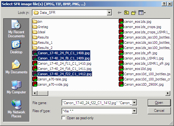
File selection
|
| RAW files Imatest can analyze Bayer raw files: standard files (TIFF, etc.) that contain undemosaiced data. RAW files are not very useful for measuring MTF because the pixel spacing in each image planes is twice that of the image as a whole; hence MTF is lower than for demosaiced files.(An excetion: white-balanced Bayer RAW files can be treated as standard monochrome files for MTF measurement.) But Chromatic aberration can be severely distorted by demosaicing, and is best measured in Bayer RAW files (and corrected during RAW conversion). Details of RAW files can be found here. |
Settings
Setup window
When the file (or files) have been opened, the Setup window, shown below, appears. This window allows you to select groups of regions (ROIs) for analysis, shown as violet rectangles. It also lets you select the size of the regions, whether to analyze vertical or horizontal edges, and change several additional settings. Pressing the button on the left opens the SFRplus Settings & options window, which allows you to select additional settings that affect the calculations, display, and output (for automated SFRplus runs). The light yellow-orange rectangles are for calculating the color/lightness uniformity profiles.
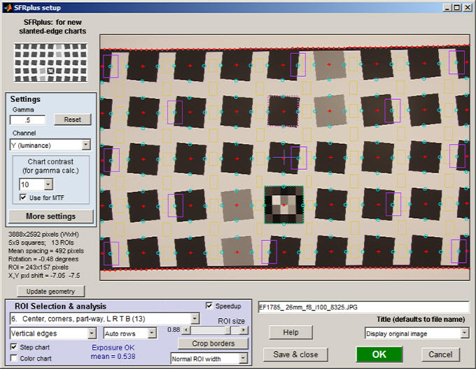
SFRplus parameters & setup window; 9 regions selected for analysis
| SFRplus setup window controls Settings | |
| Settings area | |
| Gamma | Assumed Gamma (contrast) of the chart. Has a moderate effect on the MTF results. Default is 0.5. |
| Channel | Select channel to analyze: R, G, B, Y, R-only, G-only, B-only, Y-only. (Y is Luminance channel). Use one channel only to speed up calculations or where other channels are dark and may not contain valid data. |
| Chart contrast
(for gamma calc.) |
Chart contrast– for the contrasty squares (i.e., most of them). Used to estimate gamma from the image. |
| Use for MTF | (Checkbox, normally unchecked) When checked, use the gamma derived from the chart for the MTF calculation. The correct chart contrast must be entered. This may result in a small improvement in accuracy. |
| Open the SFRplus settings window, shown below. | |
| ROI selection area | |
|
Region (center, etc) (Selects which regions to locate. Actual ROIs are located automatically) Only the recommended settings are shown. For full selection, see Using Rescharts Slanted-edge modules Part 2. |
Select the regions (ROIs) to analyze. Choices below. The number of regions is in parentheses. This is a particularly important setting. We encourage users to become familiar with the settings below. Note that the squares above and below the middle square are never selected for analysis; they are reserved for other purposes (stepchart, color chart, and/or focusing pattern). At least 13 regions are recommended for 3D plots. These selections are indicated by , below.
3. Center, corners, part-way (9) (Part-way on diagonal between center & corners). This setting is often a good compromise between speed and detail. 6. Center, corners, part-way, L, R, T, B (13) This is the smallest selection that can be used with 3D displays. 7. 5 rows, 5 columns (except step & color ROIs) (23) (edges on a 5×5 grid, omitting the squares above and below the middle). Highly detailed results, well-suited for 3D displays. 10. All squares, inner & boundary edges (best 3D map). A highly detailed grid, recommended for detailed 3D displays. The edges tend to be non-overlapping. Best for 3D plots where squares have a single contrast. 13. All squares, inner & bdry except low contrast (good 3D map). A highly detailed grid, recommended for detailed 3D displays for charts that have two contrast levels (mostly high (10:1) and a few low (2:1)). The edges tend to be non-overlapping. Best for 3D plots with charts that have squares with two contrast levels. |
| Vertical, Horizontal edges (or Both) | Selects Vertical edges, Horizontal edges, or Both. Usually Vertical, but Horizontal or Both is often useful. Use Both for Lens-style MTF plots. |
| Step chart (checkbox) | Perform step chart analysis. Should be checked when the grayscale stepchart is present. Checked by default. |
| Color chart (checkbox) | Perform color analysis. Only if color pattern is included. Not needed for lens testing. |
| Rows
(Auto or number) |
The number of rows of squares in the chart (between the top and bottom bars) or Auto for automatic row detection (the default). Normally Auto, but may need to be set to the actual number of rows when Auto fails (e.g., when the aspect ratio of the squares is not 1:1).. |
| Negative | Check this box for negative images (light squares on dark background). |
| Speedup (checkbox) | Checked recommended. Eliminates some calculations not needed for lens testing, including noise histograms and SQF. |
| ROI size | Slider that determines the size of the ROI. Use the largest value that keeps a save distance from edges of squares and top and bottom bars.0.8 to 0.9 is typical. May need to be smaller where distortion is severe. |
| Allows borders to be cropped to remove interfering patterns that might otherwise be included in the image. This button is tinted pink whenever the image is cropped. | |
| ROI width
(below ROI size slider) |
Width of ROI selection. Normal width for the standard rectangular ROI. Choose Wider or Widest for very fuzzy edges. |
| Other controls | |
| Title | Title. Defaults to file name. You can add a description. |
| |
Open this web page in a web browser. |
| Image setting | Selects image channel for display: Original (RGB) image, Red, Green, or Blue channels. |
| Save settings (for use in auto SFRplus), but do not continue with run. | |
| Save settings and continue with run: Calculate results for all selected region. You will be able to view results interactively. | |
| Cancel run; do not save settings. | |
After you’ve finished making settings, click to save settings and continue with the run. You can click to save the settings without continuing.
Settings window
The SFRplus settings window, shown below, opens when in the setup window is pressed. The settings are saved when is pressed. Recommended settings are shown. More detail in Using Rescharts Slanted-edge modules Part 2.
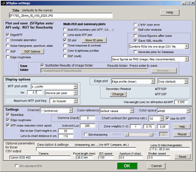
SFRplus settings window
This window is divided into sections: Title and on top, then Plot and save, Display options, Settings, Optional parameters, and finally, or .
Title defaults to the input file name. You may leave it unchanged or add descriptive information.
opens a browser window containing a web page describing the module.
|
Plot and save (for SFRplus Auto or eSFR ISO Auto and IT; NOT for Rescharts). This area selects figures to plot and save as well as a number of data save settings. It only applies to the automatic version of SFRplus in Imatest Master (also EXE and DLLs) — it is not for Rescharts. The leftmost checkboxes in this section select figures to plot and save. Note that all plotted figures are saved. Saved figures, CSV, and XML files are given names that consist of a root file name (which defaults to the image file name) with a suffix added. Examples:
Close figures after save should be checked if a large number of figures is to be displayed. It prevents a buildup of figures, which can slow processing. A CSV summary file is saved for all runs. An XML file is saved if Save XML results is checked. You can select either Save CSV files for individual ROIs or Save summary CSV file only (the summary file is always saved). Save figures as PNG or FIG files. PNG files (a losslessly-compressed image file format) are the default—.they require the least storage. Matlab FIG files allow the data to be manipulated– Figures can be resized, zoomed, or rotated (3D figures-only). FIG files should be used sparingly because they can be quite large. PNG files are preferred if no additional manipulation is required. Save folder determines where results are stored. It can be set either to subfolder Results of the image folder or to a folder of your choice. Subfolder Results is recommended because it is easy to find if the image folder is known. When 3D plot is checked, SFRplus Auto plots the last 3D plot displayed in Rescharts unless the button has been pressed and one or more plots has been selected. will be displayed in pink in this case. This allows several 3D plots to be displayed and saved by SFRplus auto. |
|
Display options contains settings that affect the display (units, appearance, etc.). MTF plots (individual and summary) selects the spatial frequency scale for MTF plots for for the summary plot. Cycles/pixel (C/P), Cycles/mm (lp/mm), Cycles/inch (lp/in), Line Widths per Picture Height (LW/PH), and Line Pairs per Picture Height (LP/PH) are the choices. (Note that one cycle is the same as one line pair or two line widths.) If you select Cycles per inch or Cycles/mm, you must enter a number for the pixel size— either in pixels per inch, pixels per mm, or microns per pixel. For more detail on pixel size, see the box below. Maximum MTF plot frequency selects the maximum display frequency for MTF plots. The default is 2x Nyquist (1 cycle/pixel). This works well for high quality digital cameras, not for imaging systems where the edge is spread over several pixels. In such cases, a lower maximum frequency produces a more readable plot. 1x Nyquist (0.5 cycle/pixel), 0.5x Nyquist (0.25 cycle/pixel), and 0.2x Nyquist (0.1 cycle/pixel) are available. Chart contrast For a medium or low contrast charts (contrastgamma will be calculated and displayed along with the contrast factor (the chart contrast multiplier = measured gamma/nominal gamma, where nominal gamma is entered in the Settings area, described below). If the Use for MTF box just to the right is checked, this value will be used in the MTF calculation, which may result in a modest improvement in accuracy.
|
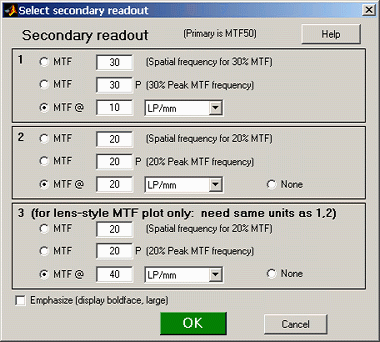
Secondary readout controls the secondary readout display in MTF plots. The primary readout is MTF50 (the half-contrast spatial frequency). Two secondary readouts are available with several options. The first defaults to MTF30 (the spatial frequency where MTF is 30%). The third is used only for SFRplus Lens-style MTF plots.
Clicking Change opens the window shown on the right. Secondary readout settings are saved between runs. Choices:
-
The upper radio button (MTF) for each readout selects MTFnn, the spatial frequency where MTF is nn% of its low frequency value.
-
The middle radio button selects MTFnnP, the spatial frequency where MTF is nn% of its peak value: useful with strongly oversharpened edges.
-
The lower radio button (MTF @ ) selects MTF @ nn units, where nn is a spatial frequency in units of Cycles/pixel, LP/mm, or LP/in. If you select this button, the pixel spacing should be specified in the Cycles per… line in the Plot section of the input dialog box, shown above. A reminder message is displayed if the pixel spacing has been omitted.
Edge plot selects the contents of the upper (edge) plot. The edge can be cropped (default) or the entire edge can be displayed. Three displays are available.
- Edge profile (linear) is the edge profile with gamma-encoding removed. The values in this plot are proportional to light intensity. This is the default display.
- Line spread function (LSF) is the derivative of the linear edge profile. MTF is the fast fourier transform (FFT) of the LSF. When LSF is selected, LSF variance (σ2), which is proportional to the DxO blur unit, is displayed.
- Edge pixel profile is proportional to the edge profile in pixels, which includes the effects of gamma encoding.
|
Settings affect the calculations as well as the display. Gamma is used to linearize the input data, i.e., to remove the gamma encoding applied in the camera or RAW converter (more explanation). It defaults to 0.5 = 1/2, which is typical of digital cameras, but is affected by camera or RAW converter contrast settings. It should be set to 0.45 when RAW images are read into Imatest (to be converted by dcraw), but there is little loss in accuracy if it is left at 0.5. If is is set to less than 0.3 or greater than 0.8, the background will be changed to pink to indicate an unusual (possibly erroneous) selection. Since SFR sharpness measurements are moderately sensitive to the Gamma setting (a 10% error in gamma results in a 2.5% error in MTF50 for a normal contrast target), it’s a good idea to run Colorcheck or Stepchart to determine the correct value of Gamma. A nominal value of gamma should be entered, even if the value of gamma derived from the chart (described above) is used to calculate MTF. Channel is normally left at it’s default value of Y for the luminance channel, where Y = 0.3*R + 0.59*G + 0.11*B. In rare instances the R, G, and B color channels might be of interest. Zone weights Weights of the center, part-way, and corner zones. Used for calculating weighted means of key results. Incident lux (for ISO sensitivity calculations) When a positive value of incident light level (not blank or zero) in lux is entered in this box, ISO sensitivity is calculated and displayed in the Stepchart noise detail figure. More details are on the ISO Sensitivity and Exposure Index page. Standardized sharpening Leave unchecked for lens testing. If the checkbox is checked, standardized sharpening results are displayed as thick red curves. See SFR instructions for more details. Reset restores the settings in Options and Settings to their default values. |
|
Additional parameters (all optional) for Excel .CSV output contains a detailed description of the camera, lens, and test conditions. EXIF data is entered, if available, but can be overridden by manual settings. The Reset button clears all entries. |
When entries are complete, click to return control to the SFRplus settings & options window. When all entries are complete, click either , , or . saves the settings for use in automated SFRplus runs, which can be initiated from the button in the main Imatest window. saves the settings then calculates results for interactive viewing. A sequence of Calculating… boxes appear to let you know how calculations are proceeding. When calculations are complete, results are displayed interactively in the Rescharts window, as shown below.
Warnings
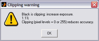
| A Clipping warning is issued if more than 0.5% of the pixels are clipped (saturated), i.e., if dark pixels reach level 0 or light pixels reach the maximum level (255 for bit depth = 8). This warning is emphasized if over 5% of the pixels are clipped. Clipping reduces the accuracy of SFR results. It makes measured sharpness better than reality. |
 |
|
|
The percentage of clipped pixels is not a reliable index of the severity of clipping or of MTF measurement error. For example, it is possible to just barely clip a large portion of the image with little loss of accuracy. The plot on the right illustrates strong clipping, indicated by the sharp corner near the “shoulder” on the black line. The MTF measurement is better than reality. The absence of a sharp corner indicates that there is little MTF error. Clipping can usually be avoided with a correct exposure— neither too dark nor light— and by avoiding high contrast targets (like the old ISO-12233 chart). The maximum recommended edge contrast is 10:1; 4:1 contrast (recommended in the upcoming revision to the ISO-12233 standard) is even better. Low-contrast targets are more reliable overall: in addition to better exposure latitude (reduced risk of clipping), they tend to have less sharpening in cameras with variable signal processing, and MTF results are less sensitive to errors in estimating gamma. |
Clipping warnings |

The following table lists figures and Excel-readable CSV files produced by Imatest SFRplus when the button is pressed.
(default location: subfolder Results)
| Excel .CSV (ASCII text files that can be opened in Excel) | |
| SFR_cypx.csv | (Database file for appending results: name does not change). Displays 10-90% rise in pixels and MTF in cycles/pixel (C/P). |
| SFR_lwph.csv | (Database file for appending results: name does not change). Displays 10-90% rise in number/Picture Height (/PH) and MTF in Line Widths per Picture Height (LW/PH). |
| filename_YA17_MTF.csv or | Excel .CSV file of MTF results for this region (designated by location (YA17) or sequence (nn = 01,…). All channels (R, G, B, and Y (luminance) ) are displayed. |
| filename_Y_multi.csv | Excel .CSV file of summary results for a multiple ROI run. |
| filename_Y_sfrbatch.csv | Excel .CSF file combining the results of batch runs (several files) with multiple ROIs. Only for automatic SFRplus (not Rescharts). Used as input to Batchview. |
Interpret the results
Sharpness is the most important (but not the only) lens measurement. To learn more about sharpness measurements, see Sharpness: What is it and how is it measured?, SFR Results: MTF (Sharpness) plot, and Rescharts Slanted-Edge Modules Part 3: Edge Results.
Remember, in evaluating lenses, use the results without standardized sharpening. The Standardized sharpening box should be unchecked. Results with standardized sharpening do, however, have some interest: they indicate what can be achieved after sharpening. But they tend to “flatten” differences between lenses.
The illustration below shows the Rescharts SFRplus window with the Edge and MTF plots for a region near the center. (Any region may be selected.) MTF50 (the spatial frequency where MTF drops to half its low frequency value) or MTF50P (the spatial frequency where MTF drops to half its peak value) are the most valuable results for lens testing: they correlate better with perceived image sharpness than any other measurements. They have the same value except when heavy sharpening is applied, in which case MTF50P is a little lower, and also more representative of the system. In general, heavy sharpening should be avoided when testing lenses. Signal processing (which includes sharpening) should be as consistent as possible.
MTF is preferred over edge response parameters (such as the 10-90% rise distance) because system MTF is the product of the MTF of individual components. No such simple formula is available for edge responses. MTF can be displayed in a number of different ways (in detail for a single region or a map of the whole image surface). Additional output parameters, for example MTF at a specified spatial frequency, can be displayed using the Secondary readout.
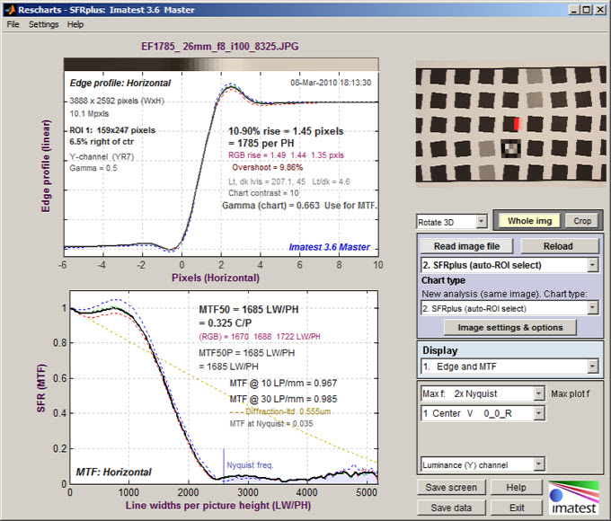
Imatest Rescharts window showing Edge and MTF plot for a single region (near the center)
Diffraction-limited MTF is shown as a pale brown dotted line when pixel spacing had been entered.
MTF curves and Image appearance contains several examples illustrating the correlation between MTF curves and perceived sharpness.
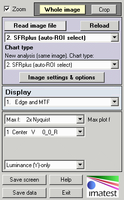
Rescharts control area
The Rescharts window has some common features for all displays.
Zoom turns zoom on and off. For 3D plots it toggles a rotate function.
The Whole image or a Crop may be displayed on the upper right.
reads a file of the type specified by Chart type below. Changing the type reads another file.
New analysis (same image) lets you reanalyze the same image with the same or different Rescharts module.
opens the Settings window, described above.
Display lets you select the display. Several are of interest for lens testing, including 1. Edge and MTF, 2. Chromatic Aberration, 3. SQF, 4. Multi-ROI summary, 12. 3D plots, and 13. Lens style MTF plot. Several will be shown below.
The options area below the Display region depends on the Display setting. Details in Rescharts Slanted-edge results Part 3.
saves and optionally displays the Rescharts window.
saves several results in CSV and XML files, shown below.
(default location: subfolder Results)
| Excel .CSV (ASCII text files that can be opened in Excel) | |
| SFR_cypx.csv | (Database file for appending results: name does not change). Displays 10-90% rise in pixels and MTF in cycles/pixel (C/P). |
| SFR_lwph.csv | (Database file for appending results: name does not change). Displays 10-90% rise in number/Picture Height (/PH) and MTF in Line Widths per Picture Height (LW/PH). |
| filename_YA17_MTF.csv or filename_nn_MTF.csv | Excel .CSV file of MTF results for this region (designated by location (YA17) or sequence (nn = 01,…). All channels (R, G, B, and Y (luminance) ) are displayed. |
| filename_Y_multi.csv | Excel .CSV file of summary results for a multiple ROI run. |
| filename_Y_sfrbatch.csv | Excel .CSF file combining the results of batch runs (several files) with multiple ROIs. Only for automatic SFRplus (not Rescharts). Used as input to Batchview. |
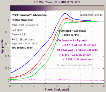
Chromatic aberration is best measured on tangential (i.e., vertical) edges near the corners. The plot shows the three channels. A key result is CA (area), which is equal to the area between the highest and lowest value (works because the x-axis is pixels and the y-axis is normalized). It is most valuable as percentage of the distance from the center to the corner. Interpretation: under 0.04; insignificant. 0.04-0.08: minor; 0.08-0.15: moderate; over 0.15: serious.
Another useful result is CA (crossing), the maximum difference between center of the edges (where 0.5 is crossed). This is more closely related to lens performance, whereas the area is more closely related to perceptual color fringing (and it strongly affected by the demosaicing algorithm). For more information, see Chromatic Aberration and SFR Results: Chromatic Aberration … plot.
Multiple regions If you selected multiple regions of interest (ROIs) you can select the multi-ROI summary, shown below for 13 regions (center, corners, part-way to corners, left, right, top, and bottom). This plot can get clutterred if too many regions are selected.
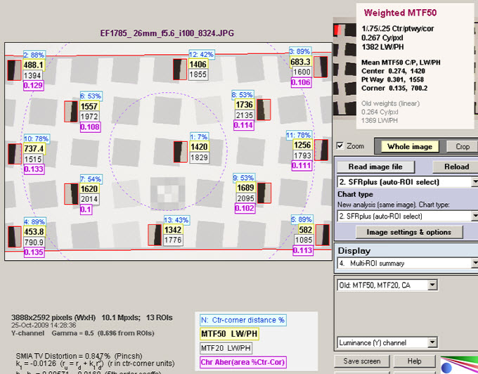
Multi-Region summary plot, showing Center-corner distances, MTF50, MTF20, and
Chromatic Aberration (in center-corner %) superimposed on image.
Distortion measurements (SMIA TV Distortion, etc.) are shown on the lower-left.
With this display you can quickly scan the summary results, then look at the detailed results for the individual region. The legend explains the four results boxes next to each ROI. The boxes contain (1) The ROI number (N) and the center-to-corner distance expressed in %, (2) MTF50 in either cycles/pixels or LW/PH, in boldface for emphasis, (3) MTF20, and (4) Chromatic Aberration (area as % of center-to-corner distance).
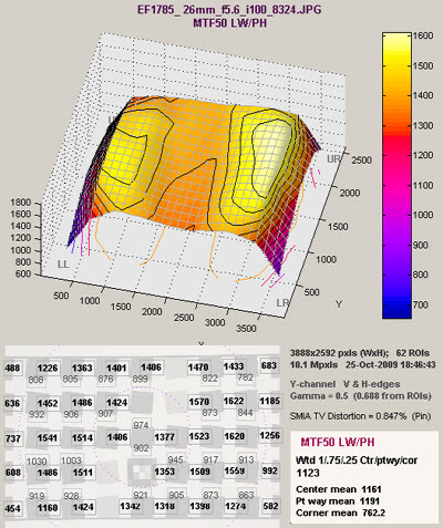
3D display (shown on right) provides the most visual detail of the results. Several options are available: a multi-region summary may be shown between the 3D plot. This display is particularly useful for locating decentering or other irregularities in the system response. MTF50 is shown, but a great many parameters may be displayed with the 3D plot. More details here.
The region selection was 13. All squares, inner & bdry except low contrast (good 3D map).
SQF— Subjective Quality Factor (not shown on this page) is a measurement of perceived display (print) sharpness that includes the contrast sensitivity of the human visual system, print size, and estimated viewing distance, in addition to MTF. Its importance will grow as it becomes more familiar. SQF is strongly affected by sharpening.
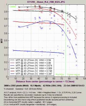
Lens-style MTF plot
Lens-style MTF plot (introduced in Imatest 3.6) This plot was designed to produce similar results to MTF plots in the Canon, Nikon, and Zeiss websites. up to three plot parameters may be selected with the Secondary readout. Typical values are 10, 20, and 40 lp/mm (used by Zeiss) or 10 and 30 lp/mm (used by Canon and Nikon).
A minimum of 13 regions is required, though more are better. Recommended region selections are 10. All squares, inner & boundary edges (best 3D map) (for single-tone charts) or 13. All squares, inner & bdry except low contrast (good 3D map) (for two-tone charts). V&H edges (both) should be selected.
Though these plots are similar to the website plots, there are several significant differences.
- Imatest calculates he system MTF, including the sensor and signal-processing. The websites display the optically-measured MTF for the lens-only. If you recognize this difference, the two sets of curves are comparable (but never identical).
- The horizontal (H) MTF curves, derived from vertical edges, are mostly radial (sagittal) near the edges (at large distances from the image center). The SFRplus chart was designed for this purpose.
- The Vertical (V) MTF curves, derived from horizontal edges, are mostly tangential (meridional) near the edges.
- The published curves assume perfect centering. Some manufacturers, like Canon, obtain their results from design calculations, not from measured test results (no centering issues!). Real lenses almost always exhibit some decentering, primarily due to manufacturing, which is more visible in other displays, particularly the 3D plots. In the lens-style MTF plot, decentering shows up as a spread in the individual readings (x for Horizontal MTF from vertical edges, • for Vertical MTF from horizontal edges).
Combining runs in batches
Once parameters have been set and saved in Rescharts SFRplus or eSFR ISO, you can run the fully automated version of SFRplus or eSFR ISO by pressing the or button in the Imatest main window. If you select a batches of files (instead of a single file), an output file with a name of the form input_filename_chan_sfrbatch.csv will be created for the Batchview program, which allows combined results to be viewed. Here is an example for six files with different apertures (f/4.5-f/22).
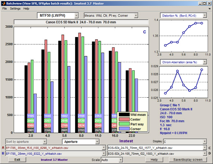
Batchview display from one set of tests: Canon 17-85mm, 26mm focal length
Two small plots (SMIA TV Distortion and Chromatic aberration area in %) and some EXIF data (metadata) from the first file in the batch are displayed on the right. Details on creating the combined file can be found in the Batchview instructions.
Checklist
License holders are encouraged to publish test results in printed publications, websites, and discussion forums, provided they include links to www. imatest.com. However you may not use Imatest for advertising or product promotion without explicit permission from Imatest LLC. Contact us if you have questions.
Imatest LLC assumes no legal liability for the contents of published reviews. If you plan to publish test results, you should take care to use good technique. This list summarizes the key points presented above. It’s well worth reviewing.
| Sturdy camera support | Use a sturdy tripod, cable release, and, for DSLRs, mirror-lock. |
| Target mounting | If you are working outdoors, be sure the target doesn’t shake in the wind. |
| Target distance | Be sure you’re far enough from the target so the printed edge quality doesn’t affect the measurements. Target distance considerations are given here. |
| Focus | Be sure the camera is focused accurately on the target. Note whether you used manual or automatic focus. |
| Target alignment | Make sure the corners, as well as the center, are in focus (challenging if the lens has significant curvature of field or the camera is misaligned). |
| Raw conversion and settings |
The choice of RAW converter (in or out of the camera) and settings, particularly Sharpening, can make a huge difference. Contrast and White balance are also important. Settings that affect contrast and transfer curve can also have a strong effect. If possible a “Linear” setting (meaning a straight gamma curve with no additional tonal response adjustments) should be used. Most important: Keep the settings consistent from run to run! |
| Gamma | SFR sharpness results are moderately sensitive to the Gamma setting: A 10% gamma error changes MTF50 by 2.5%. For best results, gamma can be measured from the grayscale stepchart in the test chart or, if the edge contrast is known, by checking “Use for MTF”. |
| Cleanliness and filters | Lens surfaces should be clean. You should note whether you have a protective (UV or Skylight) filter. It can make a difference— more likely reduced contrast than reduced sharpness. With Imatest you can find out. |
| File formats | RAW is recommended. If you use JPEG, select the highest JPEG quality. Never use less than the maximum resolution or low JPEG quality unless you are specifically testing the effects of these settings. |
| Lens settings | Lens performance is a strong function of the aperture (f-stop) and focal length (for zooms), which are included in the EXIF data in most files. They are an important part of the results. The optimum (sharpest) aperture is of particular interest (it’s typically about 2 f-stops from the maximum aperaure). Lens performance is also affected by the distance to the target if it’s very small (pay attention to chart quality for small fields of view).. |
| White balance | Should be close as possible to neutral, particularly in Colorcheck. |
Links
How to Read MTF Curves by H. H. Nasse of Carl Zeiss. Excellent, thorough introduction. 33 pages long; requires patience. Has a lot of detail on the MTF curves similar to the Lens-style MTF curve in SFRplus. Even more detail in Part II.
Understanding MTF from Luminous Landscape.com has a much shorter introduction.
Understanding image sharpness and MTF A multi-part series by the author of Imatest, mostly written prior to Imatest’s founding. Moderately technical.
Bob Atkins has an excellent introduction to MTF and SQF. SQF (subjective quality factor) is a measure of perceived print sharpness that incorporates the contrast sensitivity function (CSF) of the human eye. It will be added to Imatest Master in late October 2006.
How to Measure MTF and other Properties of Lenses by Optikos