Correlating measurement with appearance
Modulation Transfer Function (MTF) is a fundamental measure of imaging system sharpness. It is introduced in Sharpness and discussed further in Sharpening. MTF is measured by Imatest SFR, SFRplus, and by several Rescharts modules.
The most frequent questions that arise in sharpness (MTF) testing are “What does the MTF curve mean?” and “How does MTF correlate with image appearance?”
In this page we attempt to answer these questions through examples that let you quickly compare images with corresponding MTF curves by clicking on Quick links to the left of each each edge image.
Introduction
The procedure followed in this page is
- Create a reference edge whose MTF can be measured by Imatest SFR.
- Create a reference image with sharpness identical to the edge.
- Subject the edge and image to a sequence of operations that affect perceived sharpness and corresponding MTF response. These operations are performed by Picture Window Pro (an excellent reasonably-priced image editor; abbreviated below as PWP). Similar operations can be performed by Photoshop. The Blur operation closely simulates the effects of poor lens quality and misfocus.
- Display results in the individual sections below, starting with Reference.
- You can quickly switch between results for convenient comparison by clicking on the Quick Links to the left of the edge images.
The reference edge (below, left) was
- originally an SFRplus (SVG) test chart created with the Imatest Test Charts module (edge contrasts = 10:1 and 2:1),
- opened in Inkscape and exported it to a 3888 pixel wide bitmap (PNG) file,
- resized it to 50% of its original size (with very little sharpening) using Picture Window Pro,
- saved it as a PNG (losslessly compressed) file.
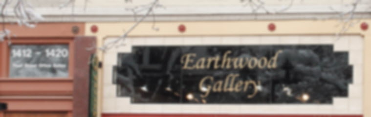
The reference image (“Earthwood Gallery”, below) was
- Taken hand-held with the Canon EOS-40D– very sharp as captured,
- Converted from a RAW image using a moderate amount of sharpening,
- resized to 50% of its original size (3888 pixels wide), then cropped,
- saved as a high quality JPEG file.
Since both images were sharp prior to resizing,
The sharpness of both images is dominated by the resize operation, i.e., they are equally sharp. The MTF plots represent both the edge and the image.
MTF plot
Note that the reference image is not “ideal” in any sense. It could have been made sharper, though this might have introduced some aliasing which would have made the slanted-edges more jagged. Sharpness is typical of Digital SLR cameras with good lenses and conservative amounts of sharpening, i.e. not oversharpened.
In the sections below, the right side of the edge and the entire image are subjected to a variety of signal processing steps: blurring (similar to what might be expected from poor quality or out of focus lenses), sharpening, and combinations of the two (similar to real-world conditions, when blurry images are sharpened). Note that sharpening increases MTF at high spatial frequencies; blurring (lowpass filtering) decreases it.
In the MTF plots, the upper plot represents the average edge response, i.e., it corresponds directly to what the eye sees on edges. The lower plot contains the MTF curve (the subject of this article!), i.e., contrast as a function of spatial frequency, expressed here in units of cycles per pixel (C/P). Note that these two curves have an inverse relationship: reducing the edge rise distance (10-90% rise) extends the MTF response (measured by MTF50).
Viewing conditions and perceived sharpness
As you observe the images on this page, keep in mind that viewing conditions strongly affect perceived sharpness— and that these images do not represent typical viewing conditions. They are reproduced full size, i.e., one image pixel occupies one screen pixe. For most digital cameras they are are crops of very large images. For example, Dell’s 20-23 inch flat screen monitors have dot pitches in the range of 0.25 to 0.28mm (91-102 pixels per inch). My 10-Megapixel Canon EOS-40D produces 3888×2592 pixel images (quite an ordinary number these days). Assuming 0.27mm pixel pitch (94 pixels per inch), total image size would be 105x70cm (41.3×27.5in); larger than most images are ever likely to be reproduced. In most cases the visual appearance corresponding to a given MTF curve will be better than what you see on this page.
Perceived sharpness of real images is dependent on image (& reproduced pixel) size, viewing distance, illumination, and the Human Visual System, whose Contrast Sensitivity function is described here.
| Setting | Description | MTF50
C/P |
MTF50P
C/P |
Over-shoot % |
| 1. Reference | A good but not perfect image; the reference for all the transformations below. Sharpness is typical of DSLRs with moderate sharpening. | 0.314 | 0.314 | 0 |
| 2. Sharpened 100% | Sharper in appearance. The small overshoot will rarely be objectionable. | 0.442 | 0.438 | 7 |
| 3. USM 100%, R=1 |
Slightly sharper then the above. Overshoot (“halo”) may be objectionable at great enlargements. | 0.448 | 0.405 | 22 |
| 4. USM 100%, R=2 |
Strongly oversharpened. The large overshoot (“halo”) is likely to be objectionable in a variety of viewing conditions. | 0.468 | 0.366 | 35 |
| 5. Blur 100% | Slight blur; typical of a mediocre lens or slight misfocus. | 0.219 | 0.219 | 0 |
| 6. Blur More 100% | Moderate blur; typical of a poor lens or poor focus. Very little response above 0.33 C/P. | 0.184 | 0.184 | 0 |
| 7. Gaussian Blur R=2 |
Strong blur; really fuzzy. Very little response above 0.2 C/P. | 0.090 | 0.090 | 0 |
| 8. Blur 100%
+ USM 100% R=1 |
Most (but not all) of the original sharpness is recovered. | 0.314 | 0.305 | 11 |
| 9. Blur More 100%
+ USM 100% R=1 |
Much of the original sharpness is recovered, but it can’t be entirely recovered because there is little contrast above 0.35 C/P. | 0.248 | 0.247 | 9 |
| 10. Gaussian Blur R=2 + USM 100% R=2 |
Sharpness is improved, but the original sharpness cannot be approached becauset contrast is nonexistent above 0.2 C/P. | 0.117 | 0.117 | 6 |
| Note: MTF50P (the spatial frequency where contrast drops to half its peak value) may be a better indicator of perceived sharpness than MTF50 (the spatial frequency where contrast drops to half its low frequency value) because it is less affected by sharpening. MTF50P differs from MTF50 only for oversharpened images. | ||||
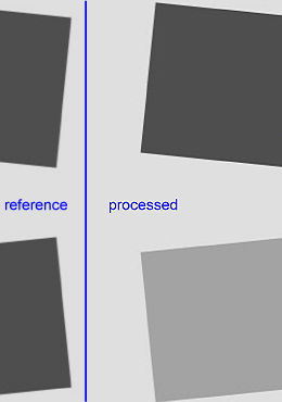
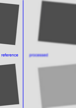
1. Reference image
| Note that the reference image is not “ideal” in any sense. It could have been made sharper, though this might have made the edges more jagged. |  |
|
| This image has no edge overshoot and only a slight hump in the MTF curve. Sharpness is typical of what you’d expect from a DSLR with a good lens and a very moderate amount of sharpening. | 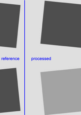 1. Reference edge |
|
| Quick Links
1. Reference
|
||

1. Reference image: This is a good, sharp image with no overshoot, typical of what a good DSLR
with conservative sharpening might produce; It is not an “ideal image”.
Sharpened images and MTF
These images have been sharpened with respect to the reference image and edge.
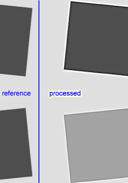
2. Sharpened
| Created using PWP’s Sharpen transformation (Amount = 100%), which uses a different algorithm from USM (Unsharp Mask). We don’t know the precise differences, but the results are visible in the MTF plots. |  |
|
|
The slight (7%) edge overshoot is unlikely to be objectionable under most viewing conditions. Image appearance is definitely improved. The overshoot corresponds to the hump in the MTF curve. |
2. Sharpen |
|
| Quick Links
1. Reference
|
||

2. Sharpened image (100%): Definitely appears sharper than the reference image; little overshoot
3. USM (Unsharp Mask) Radius = 1
| Created using PWP’s Unsharp Mask (USM) transformation (Amount = 100%, Radius = 1). Sharpening is just slightly stronger than for the Sharpen transformation (above). |  |
|
|
The edge overshoot may be somewhat objectionable in highly enlarged images. The 22% edge overshoot corresponds to a peak (1.26X) in the MTF plot. |

3. USM R=1 |
|
| Quick Links
1. Reference
|
||

3. USM Radius = 1. Slightly sharper with more overshoot (“halo”) than the sharpened image, above.
4. USM (Unsharp Mask) Radius = 2
| Created using PWP’s Unsharp Mask (USM) transformation (Amount = 100%, Radius = 2). |  |
|
|
The strong edge overshoot (“halo”) is likely to be objectionable under a variety of viewing conditions. The halo is plainly visible in the average edge (upper plot on the right). The strong halo (35% overshoot) corresponds to a peak (almost 1.5X) in the MTF curve. |
4. USM R=2 |
|
| Quick Links
1. Reference
|
||

4. USM Radius = 2. Heavy overshoot (“halo”) that may be objectionable in a variety of viewing conditions,
but an appropriate setting for images that are fuzzy to begin with.
Blurred images and MTF
This section shows the effects of blurring. MTF is representative of what you might get from mediocre lenses or poor focus.
5. Blur 100%
| Created using PWP’s Blur transformation (Amount = 100%). Typical of a mediocre lens or slight misfocus. |  |
|
|
Sharpness is moderately degraded. This might not be noticeable at small magnifications. To view the effects of sharpening on this image, click on Blur + USM R=1. |

5. Blur |
|
| Quick Links
1. Reference
|
||

5. Blur (Amount = 100%): Definitely softer than the reference image; may be acceptable at small enlargement.
Typical of a mediocre lens or slight misfocus.
6. Blur More 100%
| Created using PWP’s Blur More transformation (Amount = 100%). Typical of a poor lens or poor focus. |  |
|
|
Sharpness is moderately degraded— slightly more than for Blur. Noticeable at most magnifications. There is little contrast above 0.35 C/P. To view the effects of sharpening on this image, click on Blur More + USM R=1. |

6. Blur More |
|
| Quick Links
1. Reference
|
||

6. Blur More (Amount = 100%): slightly softer than Blur (above).
Typical of a poor lens or poor focus.
7. Gaussian Blur 100%, Radius = 2
| Created using PWP’s Gaussian Blur transformation (Amount = 100%, Radius = 2). |  |
|
|
Image sharpness is severely degraded. There is little contrast above 0.2 C/P. To view the effects of sharpening on this image, click on Gaussian Blur + USM R=2. |
7. Gaussian Blur R=2 |
|
| Quick Links
1. Reference
|
||
7. Gaussian Blur (Amount = 100%; Radius = 2): Seriously fuzzy!
Blurred then Sharpened
This section shows how sharpening (using Unsharp Mask (USM)) can recover some (but not all) of the visual degradation in blurred images.
8. Blur 100% + USM 100% Radius = 1
| Created using PWP’s Blur transformation (Amount = 100%), followed by USM (Radius = 1). The order of operations does not matter. |  |
|
|
The slight edge overshoot (11%) is unlikely to be objectionable. Image appearance is definitely improved. Most of the original sharpness is recovered. To view this image without sharpening, click on Blur. The Reference image has the same MTF50. |
 8. Blur + USM R=1 |
|
| Quick Links
1. Reference
|
||

8. Blur with USM (R = 1), which improves visual sharpness.
Much, but not quite all, of the original sharpness can be recovered.
9. Blur More 100% + USM 100% Radius = 1
| Created using PWP’s Blur More transformation (Amount = 100%), followed by USM (Radius = 1). |  |
|
|
The slight edge overshoot is unlikely to be objectionable. Image appearance is definitely improved. To view this image without sharpening, click on Blur More. |

9. Blur More + USM R=1 |
|
| Quick Links
1. Reference
|
||

9. Blur More with USM (R = 1), which improves visual sharpness.
The original sharpness cannot be recovered entirely, but the perceptual improvement may make it acceptable in many cases.
10. Gaussian Blur Radius = 2 + USM 100% Radius = 2
| Created using PWP’s Gaussian Blur transformation (Amount = 100%, Radius = 2), followed by USM (Radius = 2). |  |
|
|
The slight edge overshoot is unlikely to be objectionable. Image appearance is definitely improved, but the original sharpness cannot be recovered because there is little MTF response above 0.2 C/P. To view this image without sharpening, click on Gaussian Blur R=2. |
 10. Gaussian Blur R=2 + USM R=2 |
|
| Quick Links
1. Reference |
||

10. Gaussian blur (R = 2) with USM (R = 2), which improves visual sharpness.
The original sharpness cannot be recovered because there is little MTF response above 0.2 C/P.
Observations
- The contrast of fine features, like the text “Pearl Street Office Suites”, increases with sharpening. This is consistent with the sharpening bump or peak at medium spatial frequencies (around 0.15 to 0.25 cycles/pixel in the above examples).
- No single number extracted from the MTF curves (MTF50, MTF50P, etc.) can completely characterize perceived sharpness for all viewing conditions and all subject matter. Sharpening peaks make comparisons complex. Nevertheless, MTF50 and MTF50P are good guesses for a variety of situations.
- Sharpening cannot recover all lost sharpness. And sharpening has an additional drawback not visible on this page: it boosts noise, enough to become highly visible in some cases (DSLRs at very high ISO speeds, etc.).
- A rigorous study of Just Noticeable Difference (JND) has yet to be performed. Based on our experience, we expect the sharpness JND for MTF50 to be in the ballpark of 5%.
Sharpness ranking
Imatest’s Find Sharp Files module can produce sharpness rankings for the above files. It works on any set of similar images— not just test charts. Results are based on the absolute values of the gradients (directional derivatives) of the linearized pixel levels (yes, geeky stuff). The Sharpness numbers in the talbes below are completely arbitrary; they’re dependent on the image and crop area, i.e.,; they’re not a standard measurement and cannot be used to compare different images (or even different crops of the same image).
Sharpness ranking for crop of right side of chart images
Sharpness ranking for crop that includes most of gallery images
The Ranking is the same for the chart and gallery images and closely follows MTF50 (above), but the Sharpness numbers are (as expected) scaled differently. The Sharpness (gradient) ratios are 12.5/3.77 = 3.32 for the chart images and 27.8/7.04 = 3.95 for the gallery images. This compares with an MTF50 ratio (for the chart images) of 0.468/0.090 = 5.2.
Links
How to Read MTF Curves by H. H. Nasse of Carl Zeiss. Excellent, thorough introduction. 33 pages long; requires patience. Has a lot of detail on the MTF curves similar to the Lens-style MTF curve in SFRplus. Even more detail in Part II.
Understanding MTF from Luminous Landscape.com has a much shorter introduction.
Understanding image sharpness and MTF A multi-part series by the author of Imatest, mostly written prior to Imatest’s founding. Moderately technical.
Bob Atkins has an excellent introduction to MTF and SQF. SQF (subjective quality factor) is a measure of perceived print sharpness that incorporates the contrast sensitivity function (CSF) of the human eye. It will be added to Imatest Master in late October 2006.
How to Measure MTF and other Properties of Lenses by Optikos.