NOTE: This will be deprecated in a future release
Analyze images of the Calibrite (X-Rite) Colorchecker
Note: Colorcheck is a legacy module, no longer recommended for new work.
Use Color/Tone Interactive or Auto instead.
Introduction – Photographing the chart – Running Colorcheck – Settings – Output
Fig. 1. Grayscale tonal response & noise – Fig. 2. Noise detail – Fig. 3. a*b* color error
Saturation-corrected – FIg. 4. Color analysis – Fig. 5. Temporal noise – Saving results
|
Related: Color/Tone Interactive — Color/Tone Auto — Colorcheck/Color/Tone Appendix — Color/Tone/eSFR ISO Noise Wikipedia: Color difference |
Introduction
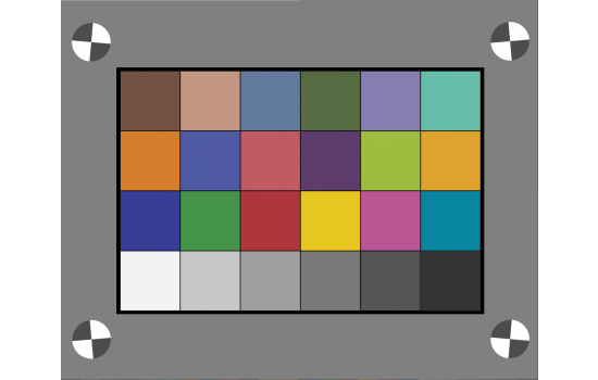
Colorcheck analyzes images of the well-known Calibrite (formerly X-RiteTM) ColorChecker®* (available from the Imatest Store) for color accuracy, white balance, tonal response (using the six grayscale patches), noise or SNR (Signal-to-Noise ratio), and ISO sensitivity. Results for tonal response are similar to Stepchart. It is particularly useful for measuring the effectiveness of White Balance algorithms and settings under a variety of lighting conditions. The ColorChecker can be photographed in isolation or as part of a scene. Algorithms and equations can be found in the Colorcheck Appendix. The ColorChecker is an 8x11″ inch chart consisting of 24 patches with 18 familiar colors and six grayscale levels with optical densities from 0.05 to 1.50; a range of 4.8 f-stops (EV). The colors are not highly saturated. The quality of the chart is very high— each patch is printed separately using carefully controlled pigments. Patches have a smooth matte surface. The smaller ColorChecker Passport is also available. It is useful for including in scenes for evaluating white balance.
*Originally introduced in 1976, it was called the Macbeth Colorchecker. After it was purchased by Gretag, it was known as the Gretag or GretagMacbeth chart. Then it moved to X-Rite, who licensed it to Calibrite in 2021. My bad joke is that you can sometimes tell a person’s age by what they call the chart.
|
The newer Color/Tone Auto; fixed, batch-capable) and Color/Tone Setup; highly interactive) modules perform all Colorcheck calculations and have a number of additional features including
We recommend these modules for new projects. Color/Tone Interactive, which has a highly interactive GUI, is useful for examining details of a camera’s color, tonal, and noise and SNR performance. Color/Tone Auto can be used as a direct replacement for Colorcheck. |
 News– Imatest 5.2: a Color Difference Visualizer (separate from Colorcheck) has been added so you can interactively examine the appearance of color differences. News– Imatest 5.2: a Color Difference Visualizer (separate from Colorcheck) has been added so you can interactively examine the appearance of color differences. |
| Version comparison | |
| Studio: | Tonal response and noise analyses for B&W patches; La*b* color error and Color analysis |
| Master: | User-supplied reference files; noise analysis for R, G, B, C, M, and Y patches; noise spectrum |
A simulated ColorChecker is shown below for sRGB color space (the Windows/Internet standard). The optical densities (–log10(reflectivity)) of the grayscale patches on the bottom row are shown in parentheses. Patch 18– Cyan– is out of the sRGB gamut; hence it can’t be reproduced perfectly on most monitors.

| 1. dark skin |
2. light skin |
3. blue sky |
4. foliage |
5. blue flower |
6. bluish green |
orange |
purplish blue |
moderate red |
purple |
yellow green |
orange yellow |
blue |
green |
red |
yellow |
magenta |
cyan |
white (.05) |
neutral 8 (.23) |
neutral 6.5 (.44) |
neutral 5 (.70) |
neutral 3.5 (1.05) |
black (1.50) |
|
Photographing the chart
-
 Good framing
Photograph the ColorChecker. The distance is not critical. There is no need to fill the frame with the ColorChecker image, especially for high resolution cameras. Filling the frame may reduce accuracy if there is significant vignetting (light falloff due to the lens system, which is often quite large in wide-angle lenses).
It may be useful to include other charts or scene elements that can affect white balance. A ColorChecker image width of 300 to 1500 pixels is sufficient for the Colorcheck noise analysis. More pixels just slow the calculations. As few as 100 (10×10) pixels per patch is adequate for color and white balance (but not noise) analysis.
The image on the right contains a ColorChecker and a Q-14 stepchart with a neutral gray surround (similar to the classic 18% gray card), which helps ensure a normal (auto) exposure. With autoexposure cameras, charts tend to be overexposed when the background is black and underexposed when it is white. Still life scenes can be used as backgrounds for testing a camera’s automatic white balance (AWB) and exposure algorithms.

Poor framing: Works, but region selection is
fussy, regions need to be very small,
and light falloff can be serious.
Margins of at least 20% of the chart height
are recommended. Backing off
will increase the available region sizes. - Lighting should be as even as possible. Lighting uniformity can be measured with an illuminance (Lux) meter. A variation of no more than ±5% is recommended. As little as possible should come from behind the camera— it can cause a reduction of contrast. An angle of incidence of about 20-45 degrees is ideal. For the noise analysis, the light should not emphasize the texture of the chart surface, which could affect noise measurements made in grayscale patches in the bottom row. More that one light source is recommended. If possible, the surroundings of the ColorChecker should be black or gray to minimize flare light. Middle gray (18-22% reflectance) is best for getting the correct exposure with auto-exposure cameras. Uneven lighting tilts the tops of the gray scale pixel plot (the upper left plot in the first figure, below). Lighting recommendations can be found in Building a Low-Cost Test Lab. If the objective of running Colorcheck is to analyze a camera’s white balance and color accuracy (and no noise analysis is required), the ColorChecker does not need to be photographed under ideal conditions. It can be part of a scene that challenges the camera’s white balance algorithm.
- If possible, the exposure should be within 1/4 f-stop of the correct value. L*a*b* color values are only accurate if exposure is correct. The exposure error is displayed in several Colorcheck figures. An explanation of exposure and grayscale levels can be found in the Colorcheck Appendix.
- Colorcheck measures the effectiveness of white balance algorithms. Results are sensitive to the type of lighting. Outdoor, flash, incandescent, and fluorescent lighting may produce different results. A Color Correction Matrix (which includes white balance) can be calculated with Color/Tone Interactive.
-
The ColorChecker may be photographed slightly out of focus to minimize errors in noise measurement due to texture in the patch surfaces. I emphasize slightly— the dark bands between the patches should remain distinct. The texture is quite low. If the lighting is reasonably diffuse (not a point source), noise from the surface texture should be minimal.
- WARNING The ColorChecker chart image should not be too large! Images over 2000 pixels wide provide no benefit and can slow calculations because Imatest uses double precision math, which consumes 24 bytes per 3-color pixel. For example, an image from a 6 megapixel camera requires 144 megabytes (6x3x8 MB) in Matlab: enough to bog down computers with limited memory. Be especially careful not to fill the frame with 8+ MB digital cameras. Save the image as a RAW file or maximum quality JPEG, then load it on your computer. If you are using a RAW converter, convert to JPEG (maximum quality), TIFF, or PNG.
Running Colorcheck
- Click on the button on the left of the Imatest main window.
- Select the file to analyze. (Imatest remembers the last folder and file name.)
|
- Crop the image. The method depends on settings that can be accessed by clicking ROI Options in the Imatest main window.
The default ROI selection method is 2. Manual coarse ROI selection; display patch squares in Fine adjustment window (Color/Tone Interactive method). Make a coarse ROI selection by dragging the cursor so a small amount of the dark boundaries are visible. Then refine the boundaries in the fine adjustment window, which is described in detail in Color/Tone Interactive. For highly distorted images like the one shown below, you can adjust the distortion slider and reduce the fill factor below the default value of 0.7. Since this image has geometrical distortion as well as strong barrel distortion, the corner positions had to be adjusted with care.
The original ROI selection method, 1. Manual coarse ROI selection; simple auto patch detection, which detects ROIs once a coarse outline has been drawn, has been deprecated in Imatest 5.0. The new automatic detection options are far superior.
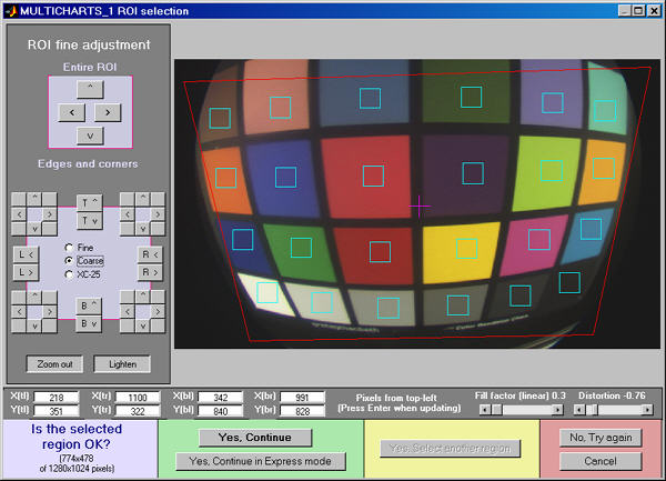
Fine adjustment of a highly distorted image. Corners, Fill factor,
and Distortion were carefully adjusted (they interact somewhat).
| This is REALLY bad framing. If there were margins around the Colorchecker equal to at least one (preferably two) patch heights, the selection would be easier, the selected squares would be larger, and results would be more accurate (with less light falloff)! |
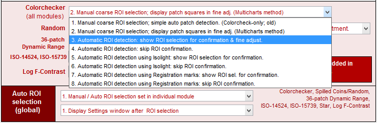
| Automatic region detection is available for the Colorchecker in all modules that support it (Colorcheck, Color/Tone Interactive, and Color/Tone Auto). Automatic region detection must be selected before running the module, by pressing in the Imatest main window. The relevant portion is shown below.
Colorchecker (all modules) ROI settings 1. The old Manual coarse ROI selection; simple auto patch detection, which only applied to Colorcheck, has been deprecated in Imatest 5.0. This selection is now the same as 2. The new automatic detection options (3 and 4) are far superior. 2. Manual coarse ROI selection; display patch squares in Fine adjustment window (Color/Tone Interactive method) (described above) is the default method. Recommended unless fully automatic detection is selected. Setting 3 is for automatic detection with the Fine Adjustment window shown after auto selection for confirmation (and adjustment, if needed). Setting 4 is for fully automatic detection without confirmation. Images with optical distortion are not handled well (as of the Beta release), but we hope to add this capability. Settings 5 and 6 are for automatic detection using the Isolight sensor buttons (just outside the corners of the Colorchecker). Faster than 3 and 4, but unable to handle optical distortion. Settings 7 and 8 are for charts with registration marks outside the Colorchecker patch area, such as the Transmissive Color Target shown on the right. Setting 9 allows auto ROI detection to use the MATLAB Colorchecker detection routine There are two dropdown menus to the right of Auto ROI selection. The first has three selections related to automatic detection: The second has two settings related to the settings window that can appear after the region selection. |
- The Imatest Colorcheck settings window appears if Express mode has not been selected. It allows you change Title, Colorchecker reference, Color space, Noise display, Color error display, and several other parameters from their default values. It also contains news about the latest updates.
| You can select either Expert or Simplified mode for the settings window. In Simplified mode many settings are grayed out so they can’t be set. If you press , commonly used settings (recommended for beginners) are selected. |
Colorcheck settings
Title: defaults to the file name. You can leave or modify it. Figure selection is in the Plot box on the right.
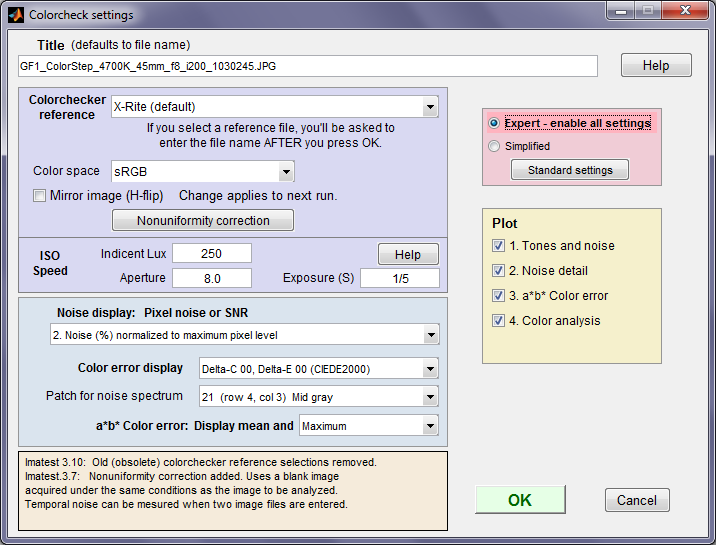 Colorcheck settings
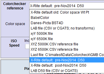
Colorchecker reference lets you select the ideal (reference) ColorChecker L*a*b* values. The order of the table is historical (the oldest settings are first) rather than logical to maintain backwards-compatibility. You can choose between any of several standard stored values (gray background below) or you can enter measured values from CSV or CGATS files (blue with pink background below). If you choose to read a reference file (L*a*b* , xyY or XYZ), a dialog box for selecting the file will appear after you press OK. The Colorchecker reference is displayed at the bottom of the L*a*b* color error figure.
Note that the cyan patch (18) is out of the sRGB color space gamut, and hence some error is expected when analyzing an ideal file (with nominal values).
|
1. X-Rite default old:
This section has been rewritten to reduce confusion. |
L*a*b* values provided by GretagMacbeth in 2005. The values are in an Excel file, Lab data Iluminate D65 & D50 spectro.xls (click on the link to open or download), that contains 2 degree D65 data used for D65 color spaces and 2 degree D50 data used for D50 color spaces. This is somewhat different from the current practice of always assuming L*a*b* data was obtained with a D50 illuminant and converting it to D65 (for D65 white point color spaces– sRGB, Adobe RGB, etc.) using a Bradford Transform. The 2 degree D50 data is still in the X-Rite Colorchecker data page (as of March 2016), even though X-Rite has announced changes to the reference values for Colorcheckers manufactured after November 2014). X-Rite default: pre-Nov 2014 D50 (described below) uses the D50 data and converts it to D65 for color spaces with a D65 white point (sRGB, etc.). |
|
2. Babelcolor |
L*a*b* values measured by Danny Pascale of Babelcolor, from Table 2 (bottom) ofRGB coordinates of the MacBeth ColorChecker, which is recommended reading for all Colorchecker users. Pascale’s D50 values are transformed to D65 using the Bradford transformation for color spaces with a D65 white point. |
|
3. Danes-Picta BST4D |
A knockoff of the Colorchecker (same geometry with different colors) from Danes-Picta in the Czech Republic (on their Digital Imaging page). |
| 4. LAB file (CSV or CGATS; no transforms) |
Read a file (CSV or CGATS format) containing L*a*b* data. The reference illuminant is assumed to be the same as the selected color space (D65 for sRGB, etc.). This is at variance with current practice, where L*a*b* files are assumed to have D50 data. The LAB D50 file is recommended. A dialog box appears for entering the filename. CSV files consist of 24 lines with L*, a*, b* values on each line separated by spaces, commas (,), or semicolons (;). Example (first 3 lines of 24): 38.08, 12.09, 14.39 66.38, 13.22, 17.14 51.06, 0.38, -22.06 (The commas are optional if spaces are present & vice-versa.) If you have an Excel .CSV file with extra rows or columns, you can easily edit it Excel by selecting the key region (3 columns, 24 rows), copying it to a new file, and saving it in .CSV format. L*a*b* data is preferred to xyY data below because it is independent of white point color temperature, hence less error-prone. The CGATS file format is also supported. |
| 5. xyY 5000K file, 6. xyY 6500K file, 7. XYZ 5000K file, 8. XYZ 6500K file |
Read a file containing xyY or XYZ data with a 5000K (D50) or 6500K (D65) white point. Procedure and format is the same is the LAB data file, above. These are generally not recommended: they are kept for backwards compatibility. |
| 9. Last file (none or file name) |
Displays the last selected reference file (LAB, xyY, or XYZ). Select to read this file. |
| 10. X-Rite default: pre-Nov 2014 D50 |
X-Rite L*a*b* D50 data for charts manufactured before November 2014, linked in the New color specifications… page, and still found on the X-Rite Colorchecker data page (as of March 2016) . Converts it to D65 for color spaces with a D65 white point (sRGB, etc.). Note that the RGB values obtained from this data do not agree with the values on the X-Rite page. Danny Pascale evidently ran into the same problem. Table 2 (top) of RGB coordinates…has two RGB columns, labeled sRGB (Pascale’s calculations) and sRGB (GMB) (from the X-Rite Colorchecker data page). The sRGB column is in agreement with Imatest sRGB values. |
| 11. X-Rite default: post-Nov 2014 D50 |
New X-Rite L*a*b* D50 data for charts manufactured after November 2014 from the New color specifications… page. Note that the CGATS files in these pages are in column-wise format, and can’t be read directly by Imatest. The post-November 2014 file uses commas (,) for decimal points. |
| 12. LAB D50 file (CSV or CGATS) |
Read a file containing D50 L*a*b* data, and transform it if needed (using a Bradford Transform) to white point the selected color space’s white point. This is the recommended approach if you have spectrophotometer measurements for your individual chart. The CSV format is described above. |
|
Reference file values can be
|
Color space allows the input file color space to be selected. The color space is automatically read into Color/Tone Interactive from the EXIF data when ExifTool has been selected in Options II; otherwise it must be entered manually. Several color spaces are available. The first six are primarily for still images. Most of the rest are for video/cinema. See the Wikipedia RGB Color Space page and brucelindbloom.com for overviews.
| sRGB | The default space of Windows and the Internet. Limited color gamut based on typical CRT phosphors. Gamma = 2.2 (approximately), White point = 6500K (D65). |
| Adobe RGB (1998) | Medium gamut, with stronger greens than sRGB. Often recommended for high quality printed output. Gamma = 2.2, White point = 6500K (D65). |
| Wide Gamut RGB | Extremely wide gamut with primaries on the spectral locus at 450, 525, and 700 microns. One of the color spaces supported by the Canon DPP RAW converter. 48-bit color files are recommended with wide gamut spaces: banding can be a problem with 24-bit color. Gamma = 2.2, White point = 5000K (D50). |
| ProPhoto RGB | Extremely wide gamut. Gamma = 1.8, White point = 5000K (D50). Described in RIMM/ROMM RGB Color Encodings by Spaulding, Woolfe and Giorgianni. |
| Apple RGB | Small gamut. Used by Apple. Gamma = 1.8, White point = 6500K (D65). |
| ColorMatch RGB | Small gamut. Used by Apple. Gamma = 1.8, White point = 5000K (D50). |
| Rec. 709 Legal | Small gamut. Used in HDTV. Pixel values 16-235. |
| Rec. 709 Full | Same as Rec. 709 Legal, but with Pixel values 0-255. |
| ACES | Academy Color Encoding System, used in the workflow developed by the folks who bring you the Oscars. Extremely large gamut, covering all visible colors. Linear gamma. White point = 6000K. |
| Rec. 2020 Legal | Fairly large gamut, covering most colors from reflected objects. For UHDTV. Pixel values 16-235. |
| Rec. 2020 Full | Same as Rec. 2020 Legal, but with Pixel values 0-255. |
| DCI-P3 | Digital cinema projection color space. 25% wider gamut than sRGB, covering most reflective surface colors. Gamma = 2.6. |
| Display p3 | Used in the iPhone 8. Same gamut as DCI-P3, but gamma is approximately 2.2 (same as sRGB). May be a part of the new Apple HEIF file format, intended to replace JPEG. This is new information (as of late 2017). Reliable information is hard to come by. |
Nonuniformity correction allows you to correct for nonuniform illumination using a separate flat field image taken under identical conditions. Opens the Nonuniformity correction window described in Nonuniformity Correction in grayscale and color chart modules.
Incident lux (for ISO sensitivity calculations) When a positive value of incident light level (not blank or zero) in lux is entered in this box, ISO sensitivity is calculated and displayed in the Stepchart noise detail figure. More details are on the ISO Sensitivity and Exposure Index page.
Noise display: Pixel noise or SNR selects the noise display for the lower-left plot of the first figure (noise/SNR for grayscale row 4) and the upper-right plot of the second figure. (noise/SNR for BGRYMC row 3). The effects of gradual illumination nonuniformities have been removed from the results. All displays are derived from Noise in pixels (the third selection below). The five display types are identical to the types in the lower noise detail plot in Stepchart. In the notation below Ni is RMS noise and Si is signal (pixel) level for patch i.
| Noise (%) normalized to White – Black (Zone 19 – 24) | 100% * (Noise in pixels) divided by (White patch (19) pixel level – Black patch (24) pixel level) \( = \frac{N}{S_{WHITE} \text{ }- S_{BLACK}} \times 100\%\). Useful because it references the noise to the scene: noise performance is not affected by camera contrast. |
| Noise (%) normalized to 255 pixels (max of 100) | \(\frac{\text{Noise in pixels}}{255} \times 100\% = N_i / 2.55\). Values 0-100. This noise measurement will be worse for higher contrast cameras. (It is affected by the gamma encoding.) |
| Noise in pixels (maximum of 255) | Noise in pixels ( Ni ). Values 0-255. |
| Pixel S/N (Signal in patch/RMS noise) dimensionless | \(\text{Signal (pixel level)} / \text{Noise} = S_i / N_i\) for each patch. Dimensionless. |
| Pixel SNR (dB) (20*log10(S/N)) | \(20 \log_{10} (\text{signal} / \text{noise})\) for each patch = \(20\log_{10}(S_i / N_i)\). Units of dB (decibels). Doubling \(\S / N\) increased dB measurement by 6.02. |
| For this selection, SNR_BW is also displayed. SNR_BW is an average SNR based on White-Black patches (Zone 19 – Zone 24; density difference = 1.45). It’s designed to be relatively independent of the chart type. (It’s calculated in Stepchart for a large variety of grayscale charts and system contrast (gamma).) \(SNR_{BW} = 20 \log_{10} \bigl( \frac{S_{WHITE} \text{ }- S_{BLACK}}{N_{mid}} \bigr)\), where Nmid is the noise in patch 22 (the 4th patch in row 4; middle gray; nominal density = 0.7). |
Color error display: Select values to be displayed as text in the upper-right of the a*b* color error figure. Wikipedia has a nice summary of color differences. You can select between
| Delta-C, Delta-E (standard (a*b*)) | CIE 1976 measurements. Geometrical distance on the a*b* plane (ΔCab) or in L*a*b* color space (ΔEab). Familiar, but not accurate for strongly chromatic colors. |
| Delta-C 94, Delta-E 94 | CIE 1994 measurements. Much more accurate for strongly chromatic colors. |
| Delta-C CMC, Delta-E CMC (1,1) | Used in the textile industry, but has has no traction in imaging. Kept for backwards compatibility. |
| Delta-C 00 Delta-E 00 (CIEDE2000) | CIEDE2000 measurements. ΔC00 and ΔE00. Recommendedas the most accurate color difference equation. See Gaurav Sharma’s CIEDE2000 Color-Difference Formula page. |
The CIE-94 and CIEDE2000 measurements reflect the eye’s reduced sensitivity to saturation differences for highly saturated colors. Mean CIE-94 numbers are typically around half of the standard 1976 measurements
Patch for noise spectrum (Imatest Master only): You can select any of the patches in the bottom two rows for calculating the noise spectrum. (Row 3 contains B, G, R, Y, M, and C primaries; row 4 contains grayscale values.) The spectra for the Y (luminance), R, G, and B channels is displayed. The third patch in row 4 (middle gray; density = 0.44) is the default.
a*b* color error: The upper-right of the a*b* color error plot displays mean color errors (ΔC… and ΔE…) and either the standard deviation of the color error (σ) or the maximum color error (max), selected in this box.
Ellipses in plot 3: Determines whether or not to display color difference ellipses on the a*b* plot. Enables you to see how a*b* differences in the reference and camera values correspond to the color difference formulas. Note that the ellipses are magnified for clarity. Choices are No ellipses, MacAdam ellipses (10x; only of historical interest), Delta-C 94 ellipses (4x), Delta-C 2000 ellipses (4x; recommended; illustrated below), and Delta-C ab circles (4x).
Plot 4 tone adjustment: The large inner square in plot 4 contains reference colors that are lightened or darkened to have a luminance comparable to the camera colors. Depending on what color model is used the color saturation may or may not be a good match to the camera values. Choices are 1. HSL (default), 2. HSV, 3. xyY, and 4. L*a*b*.
Output
The example was photographed with the Canon EOS-10D at ISO 400, and RAW converted with Canon FVU using automatic color balance.
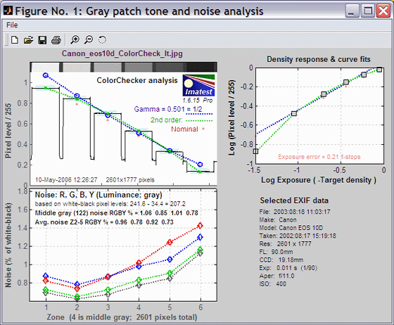
Figure 1: Gray scale tonal response and noise
shows graphic results derived from the grayscale patches in the bottom row, including tonal response and noise. Selected EXIF data is displayed, if available.
|
The upper left plot is the density response of the colorchecker (gray squares). It includes the first and second order fits (dashed blue and green lines). The horizontal axis is Log Exposure (minus the target density), printed on the back of the ColorChecker. Stepchart provides a more detailed density response curve. The exposure error is shown in pale red if it is less than 0.25 (the maximum recommended error) and bold red otherwise. Gamma (contrast) is the average slope of log pixel level as a function of log exposure ( d(log pixel level)/d(log exposure) ) for bottom row patches 2-5 (the white and black patches are excluded).
|
The upper right plot shows the noise in the third colorchecker row, which contains the most strongly colored patches: Blue, Green, Red, Yellow, Magenta, and Cyan. In certain cameras noise may vary with the color. Problems may be apparent that aren’t visible in the gray patches. Note that the x-axis scale (log exposure) is reversed from the plots on the left. |
|
The lower left plot shows the RMS noise or SNR (signal-to-noise ratio) for each patch: R, G, B, and Y (luminance). Several display options are described above. The selected display in the above figure is Noise (%) normalized to White – Black (Zone 19 – 24), i.e., RMS noise is expressed in percentage of the difference between the white and black patches.The average R, G, B, and Y noise for the gray zones (2-5) is also reported.
|
The lower right region displays EXIF data, if available. |
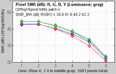
The bottom left plot has several display options, listed above. Pixel SNR (dB) is shown on the left.
\(SNR(dB) = 20 \log_{10}\bigl(\frac{S_i}{N_i}\bigr)\), where Si is the signal (mean pixel level) of patch i and Ni is the noise (standard deviation of the pixel level, with slow variations removed) of patch i.SNR_BW is an average SNR based on White – Black patches (patch 19 – patch 24; density difference = 1.45) It’s designed to be relatively independent of the chart type. (It’s calculated in Stepchart for a large variety of grayscale charts) and system contrast (gamma).)
\(SNR_{BW} = 20 \log_{10}\bigl(\frac{S_{WHITE} – S_{BLACK}}{N_{mid}}\bigr)\), where Nmid is the noise in patch 22 (the 4th patch in row 4; middle gray; closest to nominal chart density = 0.7).
| Too many open FiguresFigures can proliferate if you do a number of runs, especially SFR runs with multiple regions, and system performance suffers if too many Figures are open. You will need to manage them. Figures can be closed individually by clicking X on the upper right of the Figure or by any of the usual Windows techniques. You can close them all by clicking Close figures in the Imatest main window. Checking Close figures after save is recommended for batch runs to prevent buildup of open figures. | Clicking on Figures during calculationscan confuse Matlab. Plots can appear on the wrong figure (usually distorted) or disappear altogether. Wait until all calculations are complete— until the Save or Imatest main window appears— before clicking on any Figures. |
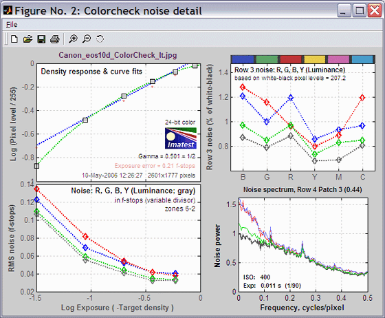
Figure 2: Noise detail (Imatest Master only)
shows the density response, noise in f-stops (a relative measurement that corresponds to the workings of the eye), noise for the third Colorchecker row, which contains primary colors, and the noise spectrum of the selected patch.
|
The upper left plot is the density response of the colorchecker (gray squares). It includes the first and second order fits (dashed blue and green lines). The horizontal axis is Log Exposure (minus the target density), printed on the back of the ColorChecker. Stepchart provides a more detailed density response curve. The exposure error is shown in pale red if it is less than 0.25 (the maximum recommended error) and bold red otherwise. ISO Sensitivity is displayed if indicent lux has been entered. Gamma (contrast) is the average slope of log pixel level as a function of log exposure ( d(log pixel level)/d(log exposure) ) for bottom row patches 2-5 (the white and black patches are excluded).
|
The upper right plot shows noise or SNR in the third Colorchecker row, which contains the most strongly colored patches: Blue, Green, Red, Yellow, Magenta, and Cyan. Several display options are described above. In certain cameras noise may vary with the color. Problems may be apparent that aren’t visible in the gray patches. |
|
The lower left plot shows the R, G, B, and Y (luminance) RMS noise for as a function of Log Exposure each patch. RMS noise is expressed in f-stops, a relative measure that corresponds closely to the workings of the human eye. This measurement is described in detail in the Stepchart tour. It is largest in the dark areas because the pixel spacing between f-stops is smallest.
|
The lower right plot shows the R, G, B, and Y noise spectrum of the selected patch. The 3rd patch in the bottom row (a middle gray) has beem selected. The spectrum conveys clues about signal processing, for example, an unusually rapid rolloff may indicate excessive noise reduction. The high levels or red and blue noise at low spatial frequencies is typical of Bayer sensors. The ISO speed and Exposure time from the EXIF data are displayed, if available. |
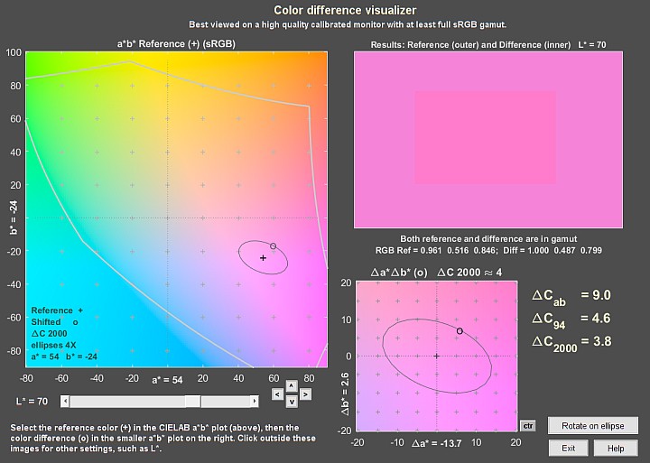
Figure 3: a*b* Color error
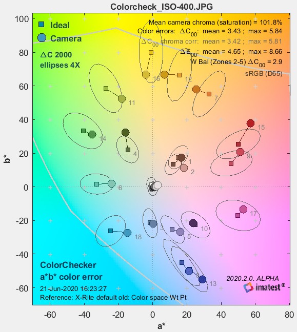 This figure illustrates color error on the a*b* plane of device-independent CIELAB color space, where a* is the horizontal axis (green-red) and b* is the vertical axis (blue-yellow). The squares are the ideal (a*, b*) ColorChecker values, selected by the ColorChecker reference setting, above. The circles are the measured (a*, b*) values. The numbers near the squares or circles correspond to the numbers of the ColorChecker patches: 1-6 are in the top row, 7-12 are in the second row, and 13-18 are in the third row. The numbers for patches 19-24 (the bottom row) are omitted because their (a*, b*) values cluster around (0, 0).
enlarged 4x.
The background of the chart shows expected colors (in monitor sRGB color space) for L* around 0.9. It presents a reasonable picture of the hues associated with a* and b* (though they shift somewhat with L*). The light gray curve is the gamut boundary of the color space (sRGB) for L(HSL) = 0.5 (CIELAB boundaries are difficult to calculate). There is significant scatter in the results because the luminance (L*) of the color patches (not displayed) varies considerably. This 2-Dimensional figure cannot display L*; a limitation is overcome in Color/Tone Interactive, which has a rotatable 3D L*a*b* display. CIELAB (often shortened to LAB) was designed to be perceptually uniform, meaning that the perceived difference between colors is approximately proportional to the Euclidian distance between them, ΔE*ab (which includes luminance L*) or ΔC* (color only; omitting L*).
\(\Delta E_{ab} = \sqrt{(L_2^* – L_1^*)^2 + (a_2^* – a_1^*)^2 + (b_2^* – b_1^*)^2}\);
\(\Delta C = \sqrt{(a_2^* – a_1^*)^2 + (b_2^* – b_1^*)^2}\)
The smallest perceptible difference corresponds roughly to ΔE*ab = ΔC = 1. (Gaurav Sharma uses 2.3 in the Digital Color Imaging Handbook, p. 31.)
CIELAB is not as perceptually uniform as originally intended. ΔEab for the minimum perceptible color difference increases with chroma (i.e., distance from the origin, (a*i2 + b*i2 )1/2. More accurate color difference difference formulas, ΔE94 and ΔE00, can be selected for display and are included in the CSV and XML output files. If you report any of the more accurate formulas, remember that they are less familiar than plain old ΔEab, so be sure to clearly indicate which formula you are using. Mean values of ΔE94 are about half of ΔEab for patches with large chroma. The relatively new CIEDE2000 color difference formula, ΔE 2000 (ΔE00), is is generally recommended. See the Colorcheck Appendix. Several values are reported on the upper right of the figure.
- Mean camera chroma (%) is the average chroma of camera colors divided by the average chroma of the ideal Colorchecker colors, expressed as a percentage. The chroma of an individual color is its distance from the origin, \(C = \sqrt{a_i^{*2}+b_i^{*2}} \). Chroma is often referred to as saturation because more chromatic colors appear to be more saturated.
\(\displaystyle \text{Mean chroma} = 100\% \times \frac{ \text{mean}\bigl( \sqrt{a_{i\_meas}^{*2} + b_{i\_meas}^{*2}}\bigr)}{\text{mean}\bigl(\sqrt{a_{i\_ideal}^{*2} + b_{i\_ideal}^{*2}}\bigr)}\) ;
i_meas denotes measured values of patch i.
i_ideal denotes ideal ColorChecker values.
Chroma is boosted when Chroma > 100%. Chroma is affected by lens quality (flare light in poor lenses decreases it) and signal processing. Many cameras and most RAW converters have adjustments for chroma (usually labelled Saturation).
Chroma is strongly affected by image processing during RAW conversion (particularly by the Color Correction Matrix (CCM)). It can be easily adjusted in image editors. Images out of cameras often have boosted saturation to make them more vivid (110-120% is common in compact digital cameras), but boosted saturation can cause a loss of detail in highly saturated objects. Saturation over 120% should be regarded as excessive.
- Chroma errors ΔCxx
Color Difference Visualizer
ΔC is color error with luminance difference omitted, i.e., color only. ΔE includes luminance difference. Imatest displays two values of ΔC: without and with correction for the saturation boost (or cut) in the camera, discussed below. You may select between three models of ΔCxx and ΔExx for the display (all are included in the CSV/XML output files).
-
- Standard ΔC and ΔE measurements (also called ΔCab and ΔEab),
- CIE 1994 measurements ( ΔC94 and ΔE94). Much more accurate,
- CIEDE2000 measurements ( ΔC00 and ΔE00). The emerging standard; the most accurate currently-available measurement. See Gaurav Sharma’s CIEDE2000 Color-Difference Formula page.
ΔC or ΔE of around 1 (2.3 according to Sharma) correspond roughly to a just noticeable difference (JND) between colors. Color difference models are described in the Colorcheck Appendix. The Color Difference Visualizer (separate from Colorcheck) in Imatest 5.2+ lets you interactively examine the appearance of color differences.
- Color error ΔC calculated with chroma (saturation) correction. This is not a standard calculation. It has been de-emphasized, and may be removed from Figure 3 in the future (but it will be kept in the CSV and JSON output).
Saturation correction involves normalizing the measured colors so their average saturation is the same as the average reference saturation. This is done by multiplying a*, b*, and C* by 100%/(Mean chroma). The corrected values, denoted by i_corr, are substituted for the measured values in the ΔC calculation.
\(\displaystyle a_{i\_corr}^* = 100 \frac{a_{i\_meas}^*}{\text{Mean chroma}}\)
\(\displaystyle b_{i\_corr}^* = 100 \frac{b_{i\_meas}^*}{\text{Mean chroma}}\)
\(\displaystyle C_{i\_corr} = \sqrt{a_{i\_corr}^{*2} + b_{i\_corr}^{*2}}\)
\(\displaystyle \Delta C_{i\_corr} = | C_{i\_corr} – C_{i\_ideal} | = \sqrt{(a_{i\_corr}^* – a_{i\_ideal}^*)^2 + (b_{i\_corr}^* – b_{i\_ideal}^*)^2}\) (Standard (CIE 1976) formula)
This normalization removes the effects of saturation boost, resulting in a lower mean color error, mean(ΔCi_corr). It is of interest because saturation can be easily adjusted by turning a (digital) knob in an image editor.
- Color error ΔExx uses the same color difference model (ab, 94, or 2000) as ΔC, above.
For the above three displays, the mean and either the maximum or the root mean square (RMS) color errors can be displayed.
mean(x) = ∑xi / n for n values of x.
RMS(x) = σ(x) = ( ∑xi2 / n )1/2 for n values of x.
x is ΔCi and ΔCi_corr for Colorchecker patches 1-18 (the top three rows).
The root mean square (RMS) error, denoted by sigma (σ), gives greater weight to large errors; it may therefore be a better overall indicator of color accuracy. You can select between σ and maximum in the input settings window.
- Summary: Figure 3 displays the mean and RMS values of the color errors, using either standard (CIE 1976), CIE 1994, or CIEDE2000 difference formulas. The latter two are more accurate, and reflect the eye’s reduced sensitivity to saturation (chroma) changes for highly saturated colors. Hence they are generally lower. The results are summarized below.
| ΔC, ΔE display summary | |||
|
One of these columns is selected.
|
The mean and RMS values of all three rows are displayed. | ||
| ΔCab | ΔC94 | ΔC00 | Color difference, omitting luminance; no saturation correction. This is the standard ΔCxx measurement. |
| ΔCab sat. corr. | ΔC94 sat. corr. | ΔC00 sat. corr. | Color difference, omitting luminance, corrected for average saturation. This is a non-standard measurement. It has been de-emphasized, and may be removed from Figure 3 in the future. |
| ΔEab | ΔE94 | ΔE00 | Color difference, including luminance; no saturation correction. |
It’s difficult to assess these numbers until a large database of test results is available. For now I would characterize the values of ΔC00 mean = 3.43 and maximum = 5.84 for the Micro Four-Thirds camera in the a*b* color error figure (above) as very good. See the Color Correction Matrix (CCM) page for more detail.
| When you interpret the results, keep the following in mind. Camera manufacturers don’t necessarily aim for accurate color reproduction, which can appear flat and dull. They recognize that there is a difference between accurate and pleasing color: most people prefer deep blue skies, saturated green foliage, and warm, slightly saturated skin tones. Ever mindful of the bottom line, they aim to please. Hence they often boost saturation, especially in blues, greens, and skin tones. |
See Links, below, for details on CIELAB color space.
Figure 4: Color analysis
is an image of the ColorChecker that allows you to compare the actual and ideal values. It also displays White Balance error using the bottom row (the grayscale patches).
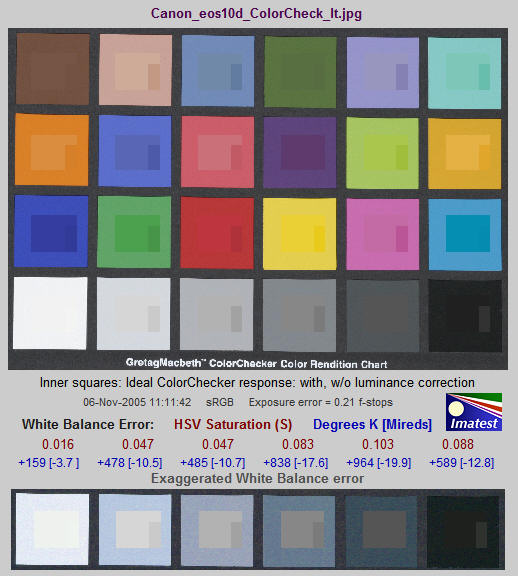
The outer portion (1) of each patch contains the ColorChecker image as photographed
The inner portion contains the ideal ColorChecker values corrected for exposure (2) and uncorrected (3).

- The outer region (zone 1) is the patch as photographed. This corresponds to the circles in the L*a*b* color error plot, above.
- The square in the center (zone 2) is the reference value of the patch, corrected for the luminance of the photographed chart. The correction is derived from the second order fit to the gray areas, described above. It is done in HSL color by default, though you can select between HSL, HSV, xyY, or L*a*b*. The average luminance of zones 1 and 2 should be close— zone 2 may be darker in some patches and lighter in others. Zones 2 and 3 correspond to the small squares (reference values) in the L*a*b* color error plot, above. The exposure error is shown on the same line as the date and color space. Best results are obtained if it is less than 0.25 f-stops.
- The small rectangle to the right of the central square, is the ideal value of the patch, without luminance correction. The luminance of zone 2 will be consistently lighter or darker than zone 3 for all patches, depending on the exposure.
In the above example, the ColorChecker image 1 is slightly underexposed; it is darker than the ideal uncorrected color 3. It is also darker than the corrected ideal color 2. This is a characteristic of this camera: it tends to darken oranges and lighten blues and cyans. This can be seen in the above right ColorChecker image, which is slightly overexposed. This image of the orange-yellow patch (row 2, column 6) has about the same luminance as the uncorrected ideal color 3, but is darker than the corrected ideal color. The uncorrected ideal value 3 in the two orange-yellow images above (the example on the left and the full chart on the right) are the same, but appear to be quite different because of the interaction of colors in the eye— an effect that should be familiar to artists and photographers.
This image provides a clear visual indication of color accuracy. The L*a*b* color error plot provides a quantitative indication.
The bottom of the fourth Colorcheck figure illustrates the White Balance error (deviation from neutral gray), which is quantified in four ways.
- ΔC2000. This is probably the most perceptually meaningful color difference metric. See the Wikipedia color differences page. It is color-space independent.
- Saturation S from the HSV color model (burgundy). S can take on values between 0 for a perfect neutral gray and 1 for a totally saturated color. The perceptual color difference corresponding to S depends on the color space.
- Correlated Color Temperature (CCT) error in Degrees Kelvin (blue), calculated from a table in Color Science: Concepts and Methods, Quantitative Data and Formulae, by Günther Wyszecki and W. S. Stiles, pp. 224-228. Color temperature in degrees K is universally used to specify lighting. Higher color temperatures are perceptually “cooler” , i.e., more blue. The CCT error is the change in illumination color temperature that would cause the measured deviation from neutral gray.
- Inverse color temperature in Mireds (micro-reciprocal degrees) (blue), where Mireds = 106/(Degrees Kelvin). A more perceptually uniform metric than CCT error. It was used to specify the strength of optical color correction filters, but isn’t used much in the digital era because such filters are rarely required.
White Balance error tends to be most visible in the gray patches (2-5 in the bottom row). It is barely visible for S < 0.02. It is quite serious for S > 0.10, particularly for the lighter gray patches.
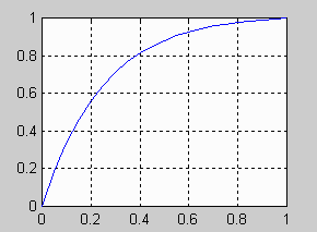
The image at the bottom shows the bottom row (the grayscale patches) with exaggerated white balance error, calculated by boosting saturation S using the curve on the left, keeping H and V constant. Low values of saturation are boosted by a factor of 4; the boost decreases as saturation increases. This image shows the White Balance error much more clearly than the unexaggerated chart. Keep it in mind that this image is worse than reality; small White Balance errors may not be obvious in actual photographs, especially in the vicinity of strongly saturated colors.
Figure 5: Temporal noise
Temporal (time-varying) noise is the random difference between otherwise identical images. It is measured as the noise (standard deviation) of the difference two identical test chart images divided by the square root of 2 (1.414).
\(N_{temporal} = \frac{\text{Noise}(\text{Image}_1 – \text{Image}_2)}{1.414}\)
Subtracting two images removes fixed pattern noise. The square root of 2 is needed because noise powers add, even though image pixels are subtracted. Dividing by the square root of 2 scales temporal noise to be the same as noise measured in an individual image.
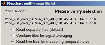
To measure temporal noise, select two images for analysis. In the dialog box shown on the right, select Read two files for measuring temporal noise. The analysis proceeds normally (for the first file), but a fourth figure, displayed if 5. Temporal noise is checked in the input dialog box Plot area, contains the temporal noise analysis. This figure is intended to be self-contained, hence repeats some features of previous plots.
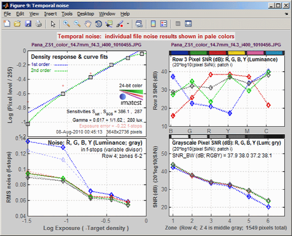
Temporal noise display
- The upper-left plot displays the density response, similar to the upper-left plot of Figure 2.
- The lower-left plot (RMS noise (f-stops)) displays scene-referenced grayscale noise or SNR using the same scale as the lower-left plot of Figure 2. In these plots, noise (or SNR) for a single image is shown as a pale curve.
- The upper-right plot (Pixel SNR (dB) for the third row (for the BGRYMC patches)) displays noise or SNR for the color patches with the scale set by Noise display in the input dialog box. It is similar to the upper-right plot of Figure 2.
- The lower-right plot (Grayscale SNR dB) displays grayscale pixel noise with the scale set by Noise display in the input dialog box (scaled the same as the lower-left plot of Figure 1 with a different x-axis).
Saving the results
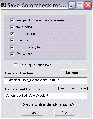
When the Colorcheck calculations are complete, the Save Colorcheck results? dialog box appears. It allows you to choose which results to save and where to save them. The default is subdirectory Results in the data file directory. You can change to another existing directory, but new results directories must be created outside of Imatest— using a utility such as Windows Explorer. (This is a limitation of this version of Matlab.) The selections are saved between runs. You can examine the output figures before you check or uncheck the boxes. After you click on Yes or No, the Imatest main window reappears. Figures, CSV, and XML data are saved in files whose names consist of a root file name with a suffix and extension. The root file name defaults to the image file name, but can be changed using the Results root file name box. Be sure to press enter. The .CSV summary file contains Excel .CSV output for the tone level, noise, and color calculations. It also contains some additional data, including EXIF data for JPEG files. The XML output file contains similar results.
Checking Close figures after save is recommended for batch runs to prevent buildup of open figures.
Summary .CSV and XML files
An optional .CSV (comma-separated variable) output file contains results for Colorcheck. Its name is [root name]_summary.csv. An example is Canon_EOS10d_ColorCheck_lt_small_summary.csv.
The format is as follows:
| Module | SFR, SFR multi-ROI, Colorcheck, or Stepchart. |
| File | File name (title). |
| Run date | mm/dd/yyyy hh:mm of run. |
| (blank line) | |
| Tables | Tables are separated by blank lines. |
| The first table contains ideal and measured pixel levels and densities. Zone is the chart patch (19-24 for grays). Gray is 1-6, corresponding to patches 19-24. Pixel is the measured pixel level (maximum = 255). Pixel/255 is the normalized measured pixel level. Px/255 ideal is the ideal normalized pixel level. Log(exp) is (-)patch density. Log(px/255) is the log exposure. WB Err Deg and WB Err Mired are white balance errors in degrees and mireds (micro reciprocal degrees), respectively. | |
| The second table contains noise measurements for the R, G, B, and Y channels for the the patches in the bottom two rows. Noise is measured in both % of the maximum density patch (19) of the Colorchecker (density = 1.5) and f-stops. | |
| The third table contains S/N and SNR (dB) measurements, described above. | |
| The fourth table contains ideal and measured RGB and La*b* values for the 24 patches. | |
| The fifth table contains several color error measurements (differences with the ideal Colorchecker values) for the 24 patches: ΔC (color difference, neglecting luminance L), ΔE (total difference, including L) using measured (camera) values with and without saturation correction. Details in the Colorcheck Appendix. | |
| (blank line) | |
| Additional data | The first entry is the name of the data; the second (and additional) entries contain the value. Names are generally self-explanatory (similar to the figures). |
| (blank line) | |
| EXIF data | Displayed if available. EXIF data is image file metadata that contains important camera, lens, and exposure settings. By default, Imatest uses a small program, jhead.exe, which works only with JPEG files, to read EXIF data. To read detailed EXIF data from all image file formats, we recommend downloading, installing, and selecting Phil Harvey’s ExifTool, as described here. |
This format is similar for all modules. Data is largely self-explanatory. Enhancements to .CSV files will be listed in the Change Log.The optional XML output file contains results similar to the .CSV file. Its contents are largely self-explanatory. It is stored in [root name].xml. XML output will be used for extensions to Imatest, such as databases, to be written by Imatest and third parties. Contact us if you have questions or suggestions.
Links
RGB coordinates of the Macbeth ColorChecker by Danny Pascale, BabelColor, 2003 (PDF). Excellent survey of color spaces and techniques for calculating the RGB values of the ColorChecker. And don’t forget his other Colorchecker page
Bruce Lindbloom Outstanding site with equations for converting between color spaces and models. Slightly different L*a*b* values from Pascale.
Earl F. Glynn (EFG) has an excellent description of the ColorChecker. His Computer Lab and Reference Library are a goldmine of information about color, image processing, and related topics.
Munsell Color Science Laboratory (at RIT) has an interesting page of color standards data available for download, including the spectral reflectivities of the Colorchecker measured by Noboru Ohta.
CIE Fundamentals for Color Measurements by Yoshi Ohno, Optical Technology Division, NIST. An excellent review of CIE colorimetry from an IS&T technical conference. Describes the CIE 1931 (x, y) and 1976 (u’v’) diagrams.
Digital Color Imaging by Gaurav Sharma A comprehensive 1997 review paper that was updated and turned into the first chapter of the Digital Color Imaging Handbook.
ColorChecker® is a trademark of X-Rite, which has apparently been licensed to Calibrite. ColorChecker L*a*b* values are supplied courtesy of X-Rite.
