Algorithms and reference formulas
This page contains algorithms and reference formulas for Colorcheck, Color/Tone Setup and Color/Tone Auto. It’s mostly in green text because it’s all math.
RGB to CIELAB (L*a*b*) – Color temperature – Color difference formulas – CIE 1976 – CIE 1994 – CIEDE2000 –
Delta-C – Color ellipses(ΔC ab, ΔC 94, ΔC 2000) – Color difference visualizer – Chroma correction (corr)
Algorithm – Grayscale and Exposure error (fix in 5.1+)
|
Background reading: We frequently get difficult questions about color spaces, color space white points, illuminants for measuring CIELAB reference files, color temperatures for measuring images, how to transform between them, and more. To help with these, strongly recommend A Review of RGB Color Spaces by Danny Pascale of Babelcolor. |
RGB to CIELAB (L*a*b)
Imatest Color/Tone measures patches in RGB images. How do we get to CIELAB?
Most images measured by imatest start their digital life as raw images in images sensors. To be useful, they are converted into interchangeable RGB image files, which usually have a color space associated with them (it may be embedded in the file). This conversion involves demosaicing, white balance, color correction (often using a Color Correction matrix), gamma-encoding, and (to varying degrees) sharpening and noise reduction. The blocks that matter in color analysis are white balance (often combined with color correction) and gamma-encoding.
RGB data is first converted to XYZ. An example of this is on the Wikipedia sRGB page. The image is linearized by inverting the gamma encoding, then a matrix is used to convert linear RGB to XYZ.
Next, XYZ data is converted to CIELAB, i.e., L*a*b*. The process is shown in the Wikipedia CIELAB color space page. The differences between the L*a*b* values of the image and the reference values (for the chart: either the default values or values read in from a reference file) are expressed with one of the color difference metrics, below. ΔE 2000 (ΔE00) and ΔC 2000 (ΔC00) are generally preferred.
|
The color reference for a test chart contains CIELAB (device-independent L*a*b*) values for each patch of the chart. It can be
Questions frequently arise regarding the color temperature used to (1) measure the patches for the reference file, (2) measure camera color accuracy from a chart image, and (sometimes forgotten), and (3) built into the color space used by the camera under test. (All interchangeable files have a color space associated with them, implicitly or explicitly.) Patches are measured with a light source with a known color temperature, typically 5000K. Color spaces have a illuminant white point. sRGB (the widely used internet Windows standard) has a 6500K illuminant white point and a D50 (~5000K) ambient (viewing environment) white point. Wikipedia does little to resolve the confusion, but the 6500K illuminant white point is the chief property of the file. A Bradford transform is typically applied to convert the 5000K measurement to the 6500K color space illuminant white point.. A frequent question is, “Is a special reference file needed for measuring charts with illuminants different from the color space white point (typically 6500K)?” The question is important because Imatest measurements (and indeed almost all camera operation) can be made with a wide variety of color temperatures, ranging from 2400K for incandescent lights to >10000K for some daylight conditions. The quick answer is “No”. The standard reference file should be used. The raw image is often transformed in the camera by an algorithm that estimates the illuminant color temperature, then applied a Color Correction Matrix to the image to white balance it and correct the colors. The CCM can also be applied to an uncorrected image by Imatest. |
Color difference (error) formulas-
You have two rectangular patches with different colors. How different are they?
The Wikipedia Color Difference page has a concise introduction to color difference concepts and equations. This page (written before the Wikipedia page was available) covers similar material.
The notation on this page is adapted from the Digital Color Imaging Handbook, edited by Gaurav Sharma, published by the CRC Press, referred to below as DCIH. The DCIH online Errata was consulted.
In measuring color error, keep it in mind that accurate color is not necessarily the same as pleasing color. Many manufacturers deliberately alter colors to make them more pleasing, typically by increasing saturation. (That is why Fujichrome Velvia was so successful when it was introduced in 1990.) In calculating color error, you may choose not to use the exact Colorchecker (or other chart) L*a*b* reference values; you may want to substitute your own enhanced values. Imatest Master allows you to enter reference values from a file written in CSV format (you can save the values from a measured chart using Color/Tone Setup).
Imatest users frequently ask about the meaning of “corr” and “uncorr” in the Colorcheck a*b* error plot. Corr means that the mean saturation (mean chroma = mean(sqrt(a*2+b*2)) of the camera is adjusted to be the same as that of the reference before making the comparison. This is a very easy correction to make; it tells how accurate the color hue would be if the mean chroma were the same as the reference. See below for more detail.
Absolute differences (including luminance)
CIE 1976
The CIELAB (L*a*b*) color space was designed to be relatively perceptually uniform. That means that perceptible color difference is approximately equal to the Euclidean distance between L*a*b* values. For colors {L1*, a1*, b1*} and {L2*, a2*, b2*}, where ΔL* = L2* – L1*, Δa* = a2* – a1*, and Δb* = b2* – b1*,
\(\Delta E^*_{ab} = \sqrt{\Delta L^{*2} + \Delta a^{*2} + \Delta b^{*2} } \) (DCIH (1.42, 5.35).
Although ΔE*ab is relatively simple to calculate and understand, it’s not very accurate, especially for strongly saturated colors. L*a*b* is not as perceptually uniform as its designers intended. For example, for saturated colors, which have large chroma values (C* = ( a*2 + b*2 )1/2 ), the eye is less sensitive to changes in chroma than to corresponding changes for Hue ( \(\Delta H^* = \sqrt{\Delta E^{*2}_{ab} – \Delta L^{*2} – \Delta C^{*2}_{ab}}\) ) or Luminance (ΔL*). To address this issue, several additional color difference formulas have been established. In these formulas, just-noticeable differences (JNDs) are represented by ellipsoids rather than circles.
CIE 1994
The CIE-94 color difference formula, ΔE*94, provides a better measure of perceived color difference than ΔE*ab .
\(\displaystyle \Delta E^*_{94} = \sqrt{(\Delta L^*)^2 + (\Delta C^*/S_C)^2 + (\Delta H^*/S_H)^2}\) (DCIH (5.37); omitting constants set to 1 ), where
SC = 1 + 0.045 C* ; SH = 1 + 0.015 C* (DCIH (1.53, 1.54) )
[ \(C^* = \sqrt{\sqrt{a_1^{*2} + b_1^{*2}} \ \sqrt{a_2^{*2} + b_2^{*2}}}\) (the geometrical mean chroma) gives symmetrical results for colors 1 and 2. However, when one of the colors (denoted by subscript s) is the standard, the chroma of the standard, Cs* = ( as*2 + bs*2 )1/2, is preferred for calculating SC and SH. The asymmetrical equation is used by Bruce Lindbloom.]
\(\displaystyle \Delta H^* = \sqrt{\Delta E^{*2}_{ab} – \Delta L^{*2} – \Delta C^{*2}_{ab}}\) (hue difference ; DCIH (5.36) )
\(\displaystyle \Delta C^*_{ab} = \sqrt{a^{*2}_1 + b^{*2}_1} \; – \sqrt{a^{*2}_2 + b^{*2}_2}\) (chroma difference))
CMC — The CMC color difference formula is used by the textile industry to match bolts of cloth, but it has not gained traction in the photographic industry. It is slightly asymmetrical: subscript s denotes the standard (reference) measurement. CMC is the Color Measurement Committee of the Society of Dyers and Colourists (UK). We mention it only reference. An early meeting of the CMC Standards Committee ΔE*CMC(l,c) = ( (ΔL* ⁄ lSL)2 + (ΔC* ⁄ cSC )2 + (ΔH* ⁄ SH )2 )1/2 (DCIH (5.37) ), where ΔE*CMC(1,1) (l = c = 1), used for graphic arts perceptibility measurements,.was also used by Imatest. SL = 0.040975 Ls* ⁄ (1+0.01765 Ls*) ; Ls* ≥ 16 (DCIH (1.48) ) = 0.511 ; Ls* < 16 SC = 0.0638 Cs* ⁄ (1+0.0131 ) + 0.638 ; SH = SC (TCMC FCMC + 1 – FCMC ) (DCIH (1.49, 1.50) ) FCMC = ( ( Cs*)4 ⁄ ( ( Cs*)4 + 1900 ) )1/2 (DCIH (1.51); TCMC = 0.56 + | 0.2 cos(hs* + 168°) | 164° ≤ hs* ≤ 345° (DCIH (1.52) ) = 0.36 + | 0.4 cos(hs* + 35 °) | otherwise ΔH* and ΔC* have the same formulas as CIE-94. |
CIEDE2000
The CIEDE2000 formulas (ΔEoo and ΔCoo ) are the best current color difference metric, and may be regarded as more accurate than the previous formulas. We omit the equations here because they are given in the Wikipedia Color Difference page and in Gaurav Sharma’s CIEDE2000 Color-Difference Formula web page. Default values of 1 are used for parameters kL, kC, and kH.
The CIE 1976 color difference metrics (ΔE*ab…) are still the most familiar. CIE 1994 is more accurate and robust, and retains a relatively simple equation. The complexity of the CIEDE2000 equations (DCIH, section 1.7.4, pp. 34-40) has slowed its widespread adoption, but it’s now the accepted standard. CIEDE2000 color difference metrics are the best choice.
Chroma differences ΔC (color differences that omit luminance difference)
Exposure errors strongly affect color differences ΔE*ab, ΔE*94, and ΔE*00. Since it is useful to look at color errors independently of exposure error, we define color differences that omit ΔL*.
\(\Delta C_{ab} = \sqrt{(\Delta a^*)^2 + (\Delta b^*)^2} = \sqrt{(\Delta E^*_{ab})^2 – (\Delta L^*)^2 } \) (This is a more general form: Delta-E with Delta-L removed.)
\(\Delta C_{94} = \sqrt{(\Delta C^* / S_C)^2 + (\Delta H^* / S_H)^2} \)
ΔC00 omits the ( ΔL’ ⁄ kLSL )2 term from the ΔE00 (square root) equation (see Sharma).
These formulas don’t entirely remove the effects of exposure error since a* and b* are affected somewhat by exposure, but they reduce it to a manageable level. Note that the ΔC definition can cause some confusion because it is different from the pure chroma difference, Δ|C*|, where chroma = |C*| = sqrt(a*2 + b*2). Δ|C*| is not suitable as a perceptual measurement because it does not include hue.
Other color differences used for Colorcheck grayscale
The bottom of the fourth Colorcheck figure illustrates the White Balance error (deviation from neutral gray), which is quantified in four ways.
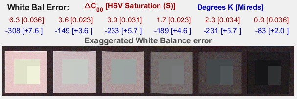
- ΔC2000. This is probably the most perceptually meaningful color difference metric. See the Wikipedia color differences page. It is color-space independent.
- Saturation S from the HSV color model (burgundy). S can take on values between 0 for a perfect neutral gray and 1 for a totally saturated color. The perceptual color difference corresponding to S depends on the color space.
- Correlated Color Temperature (CCT) error in Degrees Kelvin (blue), calculated from a table in Color Science: Concepts and Methods, Quantitative Data and Formulae, by Günther Wyszecki and W. S. Stiles, pp. 224-228. Color temperature in degrees K is universally used to specify lighting. Higher color temperatures are perceptually “cooler” , i.e., more blue. The CCT error is the change in illumination color temperature that would cause the measured deviation from neutral gray.
- Inverse color temperature in Mireds (micro-reciprocal degrees) (blue), where Mireds = 106/(Degrees Kelvin). A more perceptually uniform metric than CCT error. It was used to specify the strength of optical color correction filters, but isn’t used much in the digital era because such filters are rarely required.
Color difference representation (ellipses)
Color difference can be represented in Imatest by ΔC circles or ellipses on the a*b* plane of L*a*b* space. It can also be displayed in the xy and uv representations— useful for visualizing the perceptual uniformity of these spaces (uv isn’t as good as claimed), but a*b* is usually the best representation. Three ΔC representations are shown below (click on images to see them full size). ΔC94 and ΔC2000 are close to each other, but very different from (and superior to) ΔCab.
 ΔCab circles ΔCab circles |
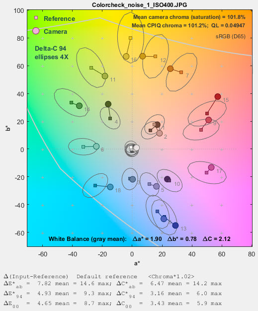 ΔC94 ellipses ΔC94 ellipses |
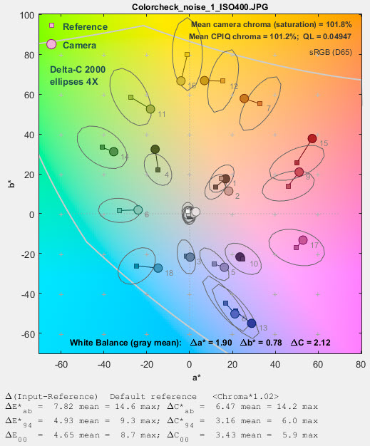 ΔC2000 ellipses ΔC2000 ellipses |
Until these ellipses were added to Imatest they were not generally available. We thought the difference between ΔC94 and ΔC2000 was greater than it actually is. In Color/Tone Setup these ellipses can be set in the Color ellipses dropdown menu. Color/Tone Auto uses settings saved from Color/Tone Setup. In Colorcheck they can be selected in the Settings window.
The White Balance (gray mean): ΔC value shown at the bottom of the plot is calculated as the mean ΔCab value of all gray scale patches with an L* value greater than 30 and less than 90.
Color difference visualizer
An app for visualizing color differences has been added to Imatest 5.2. It works best viewed on a high quality calibrated monitor with at least sRGB gamut, though it can provide information on colors on lower quality monitors. To open it from the Imatest main window, press Utility, Color Diff Visualizer or press Color Diff Visualizer in the Utility tab in the box on the right. This opens the window below with a* = b* = 0 in the large display on the left and Δa* = Δb* = 0 in the small display at the bottom, which illustrates the rotation function.
Color difference visualizer, shown for a* = 52, b* = 44, rotating on ΔC2000 ≅ 4 ellipse
To view a color difference, select an a*,b* reference value by clicking on the large a*b* display on the left. (a* and b* will be rounded to the nearest integer.) Then select Δa* and Δb* by clicking on the small display on the bottom. Color difference results are displayed on the top-right. In both the a*b* and Δa*Δb* displays + indicates the a*, b* reference value and o indicates Δa*, Δb* difference values. The selected values are displayed near the x and y-axes, respectively.
In the results display, the outer region is the a*, b* reference value (shown as magenta) and the inner part is the a*+Δa*, b*+Δb* shifted value (shown above rotating on the ΔC2000 ≅ 4 ellipse).
The small buttons with ^, v, <, and > below the right of the a*b* display shift the a* or b* setting by 1. The small ctr button to the right of the Δa*Δb* display sets Δa* = Δb* = 0.
sRGB color space is assumed. The middle gray curves in the large a*b* image represent the gamut boundaries for sRGB with L (HSL) = 0.5. Note that this is not the same as CIELAB L* = 50 (it’s more difficult to find a curve for this value).
The L* slider lets you set luminance L*.
The Rotate on ellipse button on the lower-right causes the Δa* and Δb* values to move around the ellipse. The default ellipse is for ΔC2000 = 4. You can pause or resume rotation by pressing the button. You can check (or uncheck) Fast rotation in the Settings dropdown menu. Color difference visibility may be larger during rotation than for static images because of the way the eye adapts.
The Settings dropdown lets you reset default values ( a* = Δa* = b* = Δb* =0 and L* = 70), set the axes limits in the Δa*Δb* window to ±20 (the default) or ±10, or select Fast rotation.
The Color ellipses dropdown let you set the ellipse type (none, Macadam, ΔCab, ΔC94, ΔC00 (ΔC2000) and magnification (typically 4x or 2x for the ΔC ellipses; 10x or 5x for the Macadam ellipses; 1x is just too small to be useful). ΔC2000 is the best available color difference formula, though it’s far from perfect.
Color differences corrected for chroma (saturation) boost/cut
| This result has been de-emphasized in recent versions of Imatest because adjusting chroma is not of interest to camera designers, and it is not relevant to the performance of Color Correction Matrices (CCMs). |
Many digital cameras deliberately boost chroma, i.e., saturation, to enhance image appearance in digital cameras. This boost increases color error in the ΔE* and ΔC formulas, above, though it may improve perceived image quality if it’s not overdone.
The mean chroma percentage is
Chroma(%) = 100% * (measured mean( (ai*2+bi*2)1/2 ) ) ⁄ (Colorchecker mean( (ai*2+bi*2)1/2 ) )
= 100% * mean (|Cmeasured|) ⁄ mean (|Cideal|) ; |Ci| = (ai*2+bi*2 )1/2
1 ≤ i ≤ 18 (the first three rows of the Colorchecker)
Chroma, which is closely related to the perception of saturation, is boosted when Chroma(%) > 100. Chroma boost increases ΔE* and ΔC* color error measurements. Since it is easy to remove chroma boost in image editors (with saturation settings), it is useful to measure the color error after the mean chroma has been corrected (normalized) to 100%. To do so, normalized ai_corr and bi_corr are substituted for measured (camera) values ai and bi in the above equations.
ai_corr = 100 ai ⁄ Chroma(%) ; bi_corr = 100 bi ⁄ Chroma(%)
The reference values for the ColorChecker are unchanged. Color differences corrected for chroma are denoted ΔC*ab(corr), ΔC*94(corr), and ΔC*2000(corr).
Mean and RMS values
Colorcheck Figure 3 reports the mean and RMS values of ΔC*ab corrected (for saturation) and uncorrected, where
mean(x) = Σxi ⁄ n for n values of x.
RMS(x) = σ(x) = (Σxi2 ⁄ n )1/2 for n values of x.
The RMS value is of interest because it gives more weight to the larger errors.
Colorcheck Algorithm
- Locate the regions of interest (ROIs) for the 24 ColorChecker zones.
- Calculate statistics for the six grayscale patches in the bottom row, including the average pixel levels and a second order polynomial fit to the pixel levels in the ROIs— this fit is subtracted from the pixel levels for calculating noise. It removes the effects of nonuniform illumination. Calculate the noise for each patch.
- Using the average pixel values of grayscale zones 2-5 in the bottom (omitting the extremes: white and black), the average pixel response is fit to a mathematical function (actually, two functions). This requires some explanation.
A simplified equation for a capture device (camera or scanner) response is,
normalized pixel level = (pixel level ⁄ 255) = k1 exposuregamc
Gamc is the gamma of the capture device. Monitors also have gamma = gamm defined by
monitor luminance = (pixel level ⁄ 255)gamm
Both gammas affect the final image contrast,
System gamma = gamc * gamm
Gamc is typically around 0.5 = 1/2 for digital cameras. Gamm is 1.8 for Macintosh systems; gamm is 2.2 for Windows systems and several well known color spaces (sRGB, Adobe RGB 1998, etc.). Images tend to look best when system gamma is somewhat larger than 1.0, though this doesn’t always hold— certainly not for contrasty scenes. For more on gamma, see Glossary, Using Imatest SFR, and Monitor calibration.
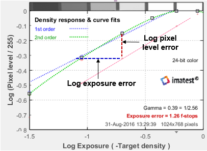
Using the equation, density = – log10(exposure) + k,
log10(normalized pixel level) = log10( k1 exposuregamc ) = k2 – gamc * density
This is a nice first order equation with slope gamc, represented by the blue dashed curves in the figure. But it’s not very accurate. A second order equation works much better:
log10(normalized pixel level) = k3 + k4 * density + k5 * density2
k3, k4, and k5 are found using second order regression and plotted in the green dashed curves. The second order fit works extremely well.
- Saturation S in HSV color representation is defined as S(HSV) = (max(R,G,B)-min(R,G,B)) ⁄ max(R,G,B). S correlates more closely with perceptual White Balance error in HSV representation than it does in HSL.
The the equation for saturation boost in the lower image of the third figure is S’ = (1-e-4S ) ⁄ (1-e-4), where e = 2.71828…
Grayscale levels and exposure error
Colorchecker grayscale patch densities (in the bottom row) are specified as 0.05, 0.23, 0.44, 0.70, 1.05, and 1.50. Using the equation,
\(\displaystyle \text{pixel level} = (10^{-density}/1.06)^{1/gamma}\)
for common gamma = 2.2 color spaces such as sRGB and Adobe RGB (see ISO sensitivity, below), the ideal pixel levels would be 236, 195, 157, 119, 83, and 52.
 Colorchecker Exposure error is measured by comparing the measured pixel levels of patches 2-5 in the bottom row (20-23 in the chart as a whole) with the selected reference levels. White and black patches 1 and 6 of the bottom row (19 and 24) are omitted because they frequently clip.
Gamma is the average slope of log pixel level vs. Log exposure, measured from patches 2-5 in the bottom row, shown on the right as a diagonal dotted blue line (·········). Pixel level is approximately proportional to exposuregamma, hence log10(exposure) is proportional to log10(pixel level) ⁄ gamma, the log exposure error for an individual patch is
\(\Delta(\text{log exposure)} = (\log_{10}(\text{measured pixel level}) – \log_{10}(\text{reference level})) / gamma\)
Using the mean value of Δ(log exposure) for Colorchecker patches 2-5 and the equation, f-stops = 3.32 * log exposure,
\(\text{Exposure error in f-stops} = 3.32 * (\text{mean}(\log_{10}(\text{measured pixel level})\, -\, \log_{10}(\text{reference level})) / gamma\)
For Stepchart and Color/Tone grayscale charts, patches with reference densities between 0.1 and 0.8 are used for calculating Exposure error.
|
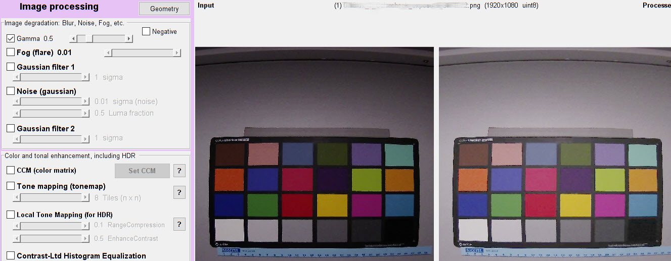
Changes to exposure error calculation in Imatest 5.1+ after December 2018 It is important to note that an image with gamma near 1 may look very dark, even though it is well-exposed. This is illustrated by the two images displayed in Image Processing, where the image on the left has gamma = 0.9 and the image on the right— derived from the image on the left (the same capture)— has gamma = 0.45.
When run in Colorcheck or Color/Tone, both images have near-zero exposure error. But you wouldn’t expect this from casually looking at the left image. |
ISO sensitivity
Two types of ISO sensitivity are calculated: Saturation-based Sensitivity and Standard Output Sensitivity. These measurements are described on the ISO Sensitivity page.
Results (CSV and JSON)
Not all results, for example, ΔH, are displayed well graphically, but they can be found in the CSV and JSON text file output. Here is a sample for the Rezchecker chart (similar colors to the Colorchecker), which can be run in Color/Tone.
JSON
“Delta_E”: [9.51,3.87,7.3,6.78,25.1,7.46,12.9,12.6,14,12.5,11.3,11.3,15.4,16.2,18.6,11.1,7.85,5.84,2.93,17.2,12.8,7.67,12.8,10.2,8.13,15.3,11.7,12.7,7.27,15.3],
“Delta_C”: [6.14,1.49,5.76,5.08,22,2.11,6.5,9.51,9.91,9.34,8.15,6.63,4.87,12.2,14.5,5.7,6.36,5.46,2.8,8.94,9.78,4.44,5.59,3.04,2.75,7.83,10.4,10.7,7.11,7.86],
“Delta_E94”: [7.97,3.64,6.06,5.22,17.2,7.22,11.4,9.42,10.3,12.2,11.2,11.2,15.4,11,12.5,11,7.65,5.8,2.91,15.6,9.7,7.59,12.7,10.1,8.11,13.4,7.91,8.18,2.74,13.7],
“Delta_C94”: [3.27,0.696,4.07,2.67,12,0.971,1.96,4.49,2.66,8.87,7.94,6.43,4.67,3,4.15,5.47,6.11,5.42,2.78,5.21,5.08,4.3,5.41,2.96,2.71,2.38,5.84,4.4,2.3,3.94],
“Delta_E2000”: [7.06,3.07,7.22,4.88,16.9,7.14,11.1,8.23,7.68,9.22,8.56,8.47,11.6,10.1,11.1,9.26,6.91,5.29,2.79,13.8,9.44,6.54,9.48,6.89,5.62,12.8,8.68,7.31,2.52,10.6],
“Delta_C2000”: [3.7,0.697,5.72,2.71,12.4,1.06,2.04,4.82,3.12,7.69,6.94,5.85,4.49,3.24,4.6,5.24,5.6,4.86,2.69,7.25,4.61,4.27,4.88,2.87,3.13,2.52,7.72,5.37,2.26,4.45],
“Delta_L”: [57.1,-7.26,-3.57,-4.48,-4.49,61.2,-12.2,48.5,84.2,85.3,79.2,-7.15,-11.2,45.9,44.8,47.1,80.4,-8.28,-9.9,-8.35,-7.85,-9.11,-14.6,-10.6,-11.8,-9.55,-4.6,2.08,-0.832,-14.7,-8.26,6.26,11.5,9.7,7.65,-13.1,51.9,-5.34,6.9,1.49,-13.2,45.8],
“Delta_Chroma”: [5.59,-6.07,1.48,-2.44,-4.45,5.11,-12.8,7.87,7.94,8.31,6.34,-2.11,-6.47,7.72,7.51,6.9,6.43,-8.38,-9.05,9.18,7.7,6,4.07,-12.1,-14.1,4.64,5.46,5.31,2.56,-0.637,-4.9,4.08,5.59,2.41,1.67,-7.77,8.4,1.63,6.55,6.49,-7.04,3.91],
“Delta_Hue_Distance”: [0,0.967,0.213,5.22,2.45,0,17.8,0,0,0,0,0.165,0.594,0,0,0,0,4.48,4.04,0,0,0,0,0.958,3.13,0,0,0,0,8.92,8.46,0,0,0,0,0.899,0,10.3,8.48,2.91,3.51,0],
“Delta_Hue_Degrees”: [0,-3.31,0.456,14,5.76,0,31.3,0,0,0,0,0.374,0.694,0,0,0,0,-8.88,3.02,0,0,0,0,-0.88,3.42,0,0,0,0,10.8,-10.3,0,0,0,0,-1.07,0,11.4,6.56,-2.6,-8.1,0],
“mean_Delta_E”: [11.5],
“mean_Delta_C”: [7.43],
“mean_Delta_E94”: [9.63],
“mean_Delta_C94”: [4.41],
“mean_Delta_E2000”: [8.34],
“mean_Delta_C2000”: [4.56],
“mean_Delta_L”: [13.7],
“mean_Delta_Chroma”: [1.39],
“mean_Delta_Hue_Distance”: [1.99],
“mean_Delta_Hue_Degrees”: [2.93],
“max_Delta_E”: [25.1],
“max_Delta_C”: [22],
“max_Delta_E94”: [17.2],
“max_Delta_C94”: [12],
“max_Delta_E2000”: [16.9],
“max_Delta_C2000”: [12.4],
“max_Delta_L”: [85.3],
“max_Delta_Chroma”: [9.18],
“max_Delta_Hue_Distance”: [17.8],
“max_Delta_Hue_Degrees”: [31.3],
CSV
| Color errors for reference vs input patches | |||||||||
| Patch | Delta-E* | Delta-C | Delta-E*94 | Delta-C 94 | Delta-E*CMC | Delta-C CMC | Delta-E 00 | Delta-C 00 | Row |
| 2 | 9.51 | 6.14 | 7.97 | 3.27 | 8.61 | 3.94 | 7.06 | 3.7 | 1 |
| 3 | 3.87 | 1.49 | 3.64 | 0.7 | 2.99 | 0.83 | 3.07 | 0.7 | 1 |
| 4 | 7.3 | 5.76 | 6.06 | 4.07 | 6.37 | 4.85 | 7.22 | 5.72 | 1 |
| 5 | 6.78 | 5.08 | 5.22 | 2.67 | 5.3 | 2.94 | 4.88 | 2.71 | 1 |
| 7 | 25.13 | 21.96 | 17.16 | 12.04 | 16.37 | 12.01 | 16.92 | 12.37 | 2 |
| 12 | 7.46 | 2.11 | 7.22 | 0.97 | 6.32 | 1.13 | 7.14 | 1.06 | 2 |
| 13 | 12.94 | 6.5 | 11.35 | 1.96 | 10.29 | 2.49 | 11.13 | 2.04 | 3 |
| 18 | 12.61 | 9.51 | 9.42 | 4.49 | 8.04 | 4.84 | 8.23 | 4.82 | 3 |
| 19 | 14.01 | 9.91 | 10.26 | 2.66 | 8.06 | 3.64 | 7.68 | 3.12 | 4 |
| 20 | 12.52 | 9.34 | 12.18 | 8.87 | 14.28 | 13.09 | 9.22 | 7.69 | 4 |
| 21 | 11.32 | 8.15 | 11.17 | 7.94 | 13.2 | 12.02 | 8.56 | 6.94 | 4 |
| 22 | 11.27 | 6.63 | 11.15 | 6.43 | 11.62 | 9.65 | 8.47 | 5.85 | 4 |
| 23 | 15.43 | 4.87 | 15.37 | 4.67 | 12.68 | 6.87 | 11.62 | 4.49 | 4 |
| 24 | 16.17 | 12.19 | 11.04 | 3 | 9.63 | 4.21 | 10.12 | 3.24 | 4 |
| 25 | 18.63 | 14.45 | 12.47 | 4.15 | 12.83 | 5.5 | 11.07 | 4.6 | 5 |
| 26 | 11.12 | 5.7 | 11.01 | 5.47 | 10.87 | 8.01 | 9.26 | 5.24 | 5 |
| 27 | 7.85 | 6.36 | 7.65 | 6.11 | 9.78 | 9.01 | 6.91 | 5.6 | 5 |
| 28 | 5.84 | 5.46 | 5.8 | 5.42 | 8.64 | 8.42 | 5.29 | 4.86 | 5 |
| 29 | 2.93 | 2.8 | 2.91 | 2.78 | 4.41 | 4.32 | 2.79 | 2.69 | 5 |
| 30 | 17.17 | 8.94 | 15.55 | 5.21 | 16.51 | 6.26 | 13.76 | 7.25 | 5 |
| 31 | 12.8 | 9.78 | 9.7 | 5.08 | 8.65 | 4.76 | 9.44 | 4.61 | 6 |
| 32 | 7.67 | 4.44 | 7.59 | 4.3 | 10.26 | 6.45 | 6.54 | 4.27 | 6 |
| 33 | 12.79 | 5.59 | 12.71 | 5.41 | 23.74 | 8.17 | 9.48 | 4.88 | 6 |
| 34 | 10.17 | 3.04 | 10.14 | 2.96 | 19.49 | 4.41 | 6.89 | 2.87 | 6 |
| 35 | 8.13 | 2.75 | 8.11 | 2.71 | 15.51 | 4.09 | 5.62 | 3.13 | 6 |
| 36 | 15.29 | 7.83 | 13.35 | 2.38 | 12.18 | 3.04 | 12.82 | 2.52 | 6 |
| 38 | 11.7 | 10.42 | 7.91 | 5.84 | 9.71 | 6.99 | 8.68 | 7.72 | 7 |
| 39 | 12.74 | 10.71 | 8.18 | 4.4 | 8.02 | 6.04 | 7.31 | 5.37 | 7 |
| 40 | 7.27 | 7.11 | 2.74 | 2.3 | 2.98 | 2.75 | 2.52 | 2.26 | 7 |
| 41 | 15.34 | 7.86 | 13.75 | 3.94 | 16.52 | 4.45 | 10.58 | 4.45 | 7 |
| Delta-E* | Delta-C | Delta-E*94 | Delta-C 94 | Delta-E*CMC | Delta-C CMC | Delta-E 00 | Delta-C 00 | ||
| Mean | 11.46 | 7.43 | 9.63 | 4.41 | 10.79 | 5.84 | 8.34 | 4.56 | |
| Maximum | 25.13 | 21.96 | 17.16 | 12.04 | 23.74 | 13.09 | 16.92 | 12.37 | |
| Additional color errors and values | |||||||||
| Patch | Delta-L* | Delta-Chroma | |Delta-Hue dist| | |Delta-Hue degs| | Note: Delta-Hue is undefined for grayscale patches (a* & b* near 0) | ||||
| 2 | 57.12 | 5.59 | 0 | 0 | |||||
| 3 | -7.26 | -6.07 | 0.97 | -3.31 | |||||
| 4 | -3.57 | 1.48 | 0.21 | 0.46 | |||||
| 5 | -4.48 | -2.44 | 5.22 | 13.97 | |||||
| 7 | -4.49 | -4.45 | 2.45 | 5.76 | |||||
| 12 | 61.23 | 5.11 | 0 | 0 | |||||
| 13 | -12.22 | -12.79 | 17.85 | 31.31 | |||||
| 18 | 48.52 | 7.87 | 0 | 0 | |||||
| 19 | 84.23 | 7.94 | 0 | 0 | |||||
| 20 | 85.25 | 8.31 | 0 | 0 | |||||
| 21 | 79.24 | 6.34 | 0 | 0 | |||||
| 22 | -7.15 | -2.11 | 0.17 | 0.37 | |||||
| 23 | -11.18 | -6.47 | 0.59 | 0.69 | |||||
| 24 | 45.95 | 7.72 | 0 | 0 | |||||
| 25 | 44.78 | 7.51 | 0 | 0 | |||||
| 26 | 47.11 | 6.9 | 0 | 0 | |||||
| 27 | 80.38 | 6.43 | 0 | 0 | |||||
| 28 | -8.28 | -8.38 | 4.48 | -8.88 | |||||
| 29 | -9.9 | -9.05 | 4.04 | 3.02 | |||||
| 30 | -8.35 | 9.18 | 0 | 0 | |||||
| 31 | -7.85 | 7.7 | 0 | 0 | |||||
| 32 | -9.11 | 6 | 0 | 0 | |||||
| 33 | -14.64 | 4.07 | 0 | 0 | |||||
| 34 | -10.62 | -12.15 | 0.96 | -0.88 | |||||
| 35 | -11.75 | -14.11 | 3.13 | 3.42 | |||||
| 36 | -9.55 | 4.64 | 0 | 0 | |||||
| 38 | -4.6 | 5.46 | 0 | 0 | |||||
| 39 | 2.08 | 5.31 | 0 | 0 | |||||
| 40 | -0.83 | 2.56 | 0 | 0 | |||||
| 41 | -14.66 | -0.64 | 8.92 | 10.84 | |||||
| Delta-L* | Delta-Chroma | |Delta-Hue dist| | |Delta-Hue degs| | ||||||
| Mean | 13.73 | 1.39 | 1.99 | 2.93 | Maximum | 85.25 | 9.18 | 17.85 | 31.31 |
| Mean camera chroma % | 107.1 | ||||||||
| Mean chroma level CPIQ % | 89.96 | ||||||||
