Noise is a random variation of image density, visible as grain in film and pixel level variations in digital images. It arises from the effects of basic physics— the photon nature of light and the thermal energy of heat— inside image sensors and amplifiers.
Noise and its measurement are introduced in Noise in photographic images.
Noise is measured by several Imatest modules. Color/tone produce the most detailed results, but noise is also measured in SFR, SFRplus, eSFR ISO, and Uniformity, and in legacy modules (no longer recommended) Stepchart and Colorcheck. ISO 15739 Visual Noise estimates the visual strength of noise using the noise spectrum, a model of the human visual system, and viewing conditions.
Imatest has a powerful Image Sensor Noise model, derived from measurements of raw images, which can be used in the Simatest Camera/Image Signal Processing Simulator to predict camera performance under a wide variety of conditions.
Noise scales strongly with pixel size. It can be very low in high quality mirrorless cameras or DSLRs, which typically have pixel sizes of at least 3 microns. But it can get ugly in cameras with tiny pixel sizes, especially at high ISO speeds or in dim light. It is also affected by sensor technology and manufacturing quality.
Software noise reduction (NR) reduces the visibility of noise by smoothing the image, excluding areas near contrasty boundaries. This technique works well, but it can obscure fine, low contrast detail. The Log Frequency-Contrast module clearly measures the effects of software noise reduction. The Random/Dead Leaves module uses a pattern that tends to maximize noise reduction (it’s the worst-case for noise reduction)— in contrast to the slanted-edge (the opposite limiting case), which tends to maximize sharpening and minimize noise reduction.
Noise in photographic images
Introduction – Noise measurements – Noise nonuniformity correction – SNR_BW – Noise appearance
Noise summary – Temporal noise – Raw vs. demosaiced noise – Noise spectrum
ISO 15739 noise and SNR – Appendix I: Scene-referenced noise, SNR, and Dynamic Range
Appendix II: The mathematics of noise – Links
|
Image Sensor Noise – measurement and modeling – using raw files for image sensor Dynamic Range and Simatest Simatest ISP/Camera Simulator — Instructions and Reference Simatest examples – Examples of how Simatest can be used. Compares simulations to measurement. Much more readable than this long page. Color/Tone / eSFR ISO Noise – including chroma, sensor (RAW), and visual noise Dynamic Range – a general introduction with links to Imatest modules that calculate it. Temporal Noise – comparing the two-image and multi-image measurements |
Introduction
Noise is a random variation of image density, visible as grain in film and pixel level variations in digital images. It is a key image quality factor; comparable in important to sharpness, and is a major factor in the Image Information Metrics (information capacity and more) used to predict machine vision system performance.
It is closely related to dynamic range— the range of brightness a camera can reproduce with good contrast and Signal-to-Noise Ratio (SNR). Since it arises from basic physics— the photon nature of light and the thermal energy of heat— it is always present. The good news is noise can be extremely low in digital cameras with large pixels (pixel pitch ≥ 3 μm). But noise can get ugly in cameras with tiny pixels, though improved signal processing in recent camera phones— such as combining multiple short images— has had remarkable success. At high ISO speeds, noise reduction software can cause a visible loss of fine detail (texture).
In most cases noise is perceived as a degradation in quality. But some Black & White photographers like its graphic effect: Many favored 35mm Tri-X film. (Film grain has very different statistics from digital noise— it’s multiplicative rather than additive, and its spectrum is dependent on density.) Pointillist painters, most notably George Seurat, created images from “noise” (specks of color) by hand; a task that can be accomplished in seconds today with Photoshop plugins. But for nearly all pictorial or technical applications, noise is undesirable.
With some recent exceptions, noise is measured from flat patches in test charts (there are many to choose from) or from flat field images. The exceptions are noise measured in sinusoidal Siemens Star and slanted edge patterns for calculationg Camera Information Capacity (a camera figure of merit that combines noise and sharpness) and related metrics.
Noise is measured by several Imatest modules: Color/Tone Interactive, Color/Tone Auto, eSFR ISO, Image Statistics, and to a limited degree in SFR, SFRplus, and Uniformity. Color/Tone Interactive, Color/Tone Auto, and eSFR ISO have the most comprehensive noise measurements. Legacy modules (Colorcheck and Stepchart) are no longer recommended.
Image Sensor Noise can be derived from measurements of raw images for use in the Simatest Camera/Image Signal Processing Simulator for predicting camera/ISP performance under a wide variety of conditions.
Noise is typically measured as RMS (Root Mean Square) noise, which is identical to the standard deviation of the flat patch signal S.
\(RMS\ Noise = \sigma(S)\), where σ denotes the standard deviation. RMS is used because \(Noise\ Power = (RMS\ Noise)^2\).
S can be the signal in any one of several color channels: R, G, B, Y (luminance, typically 0.2125 R + 0.7154 G + 0.0721 B), raw channels (R, Gr, B, Gb), or a derived channel such as R-Y or B-Y (used for chroma noise). L*, a*, b*, or others. See Color/Tone/eSFR ISO noise measurements.
Signal-to-Noise Ratio (SNR or S/N) = Signal / Noise — Since noise is only meaningful in relationship to a signal, SNR is often more useful than noise itself. SNR can be defined in many ways, depending on how Signal S is defined. For example, S can be an individual patch pixel level or the pixel difference corresponding to a specified scene density range (1.45 or 1.5 are often used for this purpose) or a difference signal for low contrast object (for Contrast Resolution SNR). It is important to know precisely how SNR is defined whenever it is discussed. SNR can be expressed as a simple ratio (S/N) or in decibels (dB), where SNR (dB) = 20 log10(S/N). Doubling S/N corresponds to increasing SNR (dB) by 6.02 dB. Most Imatest modules have several noise and SNR measurements, some simple and some detailed.
In digital cameras noise consists of two parts: fixed noise (sensor dark current noise and thermal (resistive) noise) and shot (photon) noise, which increases with the square root of the mean number of photons striking the pixels.
Noise measurements
Imatest has a method for correcting noise measurements made from unevenly illuminated patches, which can result is serious measurement errors. Since uneven illumination is very common, we describe the correction process in the box below to strongly emphasize it.
Correcting noise in patches with nonuniform illumination
|
|
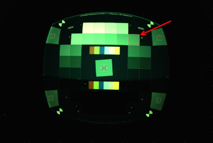
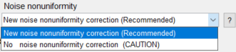
The Imatest calculation can be set in a dropdown menu in Options II and in settings windows for modules that calculate noise. We recommend New noise uniformity correction, but there is an option for turning the nonuniformity correction off (only recommended for comparison with external standard deviation calculations). When significant nonuniformity is present, it can dominate noise measurements if nonuniformity correction is not applied. The noise measurement can become strongly dependent on the size of the region (ROI). When nonuniformity correction is applied, it becomes relatively independent of region size.
For this reason, noise nonuniformity correction is absolutely critical for accurate, reliable noise measurements.
The green channel in lower left of patch 10 (closest to the image center) has a mean value of 205 (of 255). The mean value on the upper right is 160: 20% lower. Here are Image Statistics results for two different crops of the region, without and with nonuniformity correction. Similar results are observed with Color/Tone without and with nonuniformity correction (NU corr).
SNR with NU corr On is higher and also more consistent. SNR without NU corr is lower and strongly affected by region size: the smaller the region, the higher the SNR. The 13 dB difference for SNR with and without NU corr for the ~66×66 regions (which includes most of the patch) is extremely significant, as is the difference between the large and small ROIs with NU corr off. |
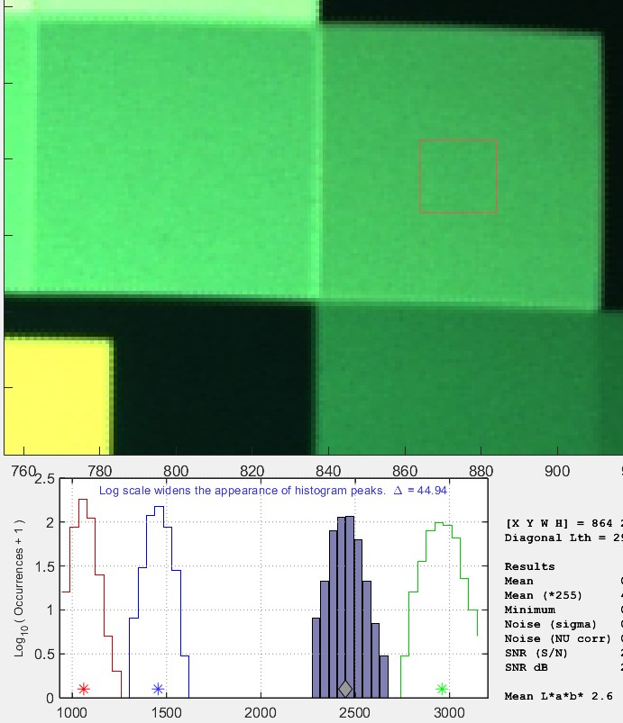 Small region and histogram 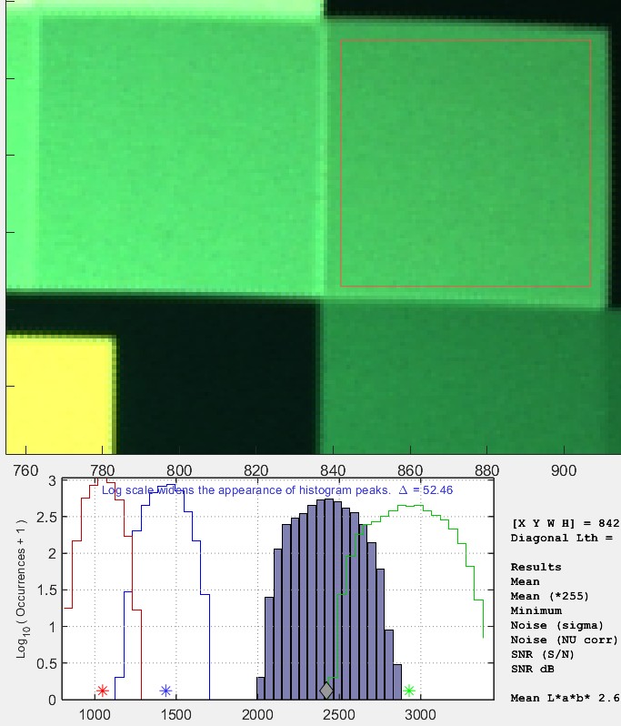 Large region and histogram, broadened by nonuniform illumination |
Noise measurements should correlate, where possible, with perceived appearance and be simple enough to interpret with minimal difficulty. There are a number of cases with additional requirements.
- For Dynamic Range calculations, noise should be referenced to the original scene so the measurement is not affected by the tonal response (gamma-encoding), which is applied in the RAW conversion process.
- For sensor performance calculations, noise should be measured from raw images (undemosaiced where possible).
Color/Tone Interactive, Color/Tone Auto, Stepchart, and Colorcheck include the following noise displays:
Noise as a function of pixel level or exposure, expressed in
-
- Pixels, normalized to the pixel difference corresponding to a scene density range of 1.5 for Stepchart (comparable to the density range of 1.45 for the GretagMacbeth ColorChecker) or the White – Black zones in the ColorChecker (row 3, patches 1 – 6; density range = 1.45). Without this normalization, noise is a function of RAW converter response curve; it increases with converter contrast.
- Pixels, normalized to the maximum pixel value: 255 for 8/24-bit files.
- Pixels (maximum of 255 for 8/24-bit files)
- f-stops (or EV or zones; a factor of two in exposure), i.e., referenced to the original scene. Noise measured in f-stops corresponds closely to human vision. See f-stop noise, below.
Noise as a simple (average) number
-
- A good single number for describing noise is the average noise of the Y (Luminance) channel, measured in pixels (normalized scene density difference of 1.5), shown in the lower plot in the figures, below. The lightest and darkest zones, representing chart densities greater than 1.5 or less than 0.1 are excluded from the average.
S/N or SNR (dB) as a function of pixel level or exposure, where S is the pixel level of the individual test chart patch.
S/N or SNR (dB) as a simple (average) number.
-
- A good single number for defining SNR is the White – Black SNR, SNR_BW, where S is the difference in pixel levels between the White and Black patches in the GretagMacbeth ColorChecker in Colorcheck (density range of 1.45), or the pixel difference corresponding to a chart (scene) density difference of 1.5 in Stepchart. Noise N is measured in a gray patch with density around 0.7. SNR_BW was developed to reduce the effect of image contrast (resulting from image processing, i.e., the application of a gamma curve) on the noise measurements.
\( SNR_{BW} = 20 \log_{10}\bigl( \frac{S_{WHITE} – S_{BLACK}}{N_{MID}} \bigr) \)
- A good single number for defining SNR is the White – Black SNR, SNR_BW, where S is the difference in pixel levels between the White and Black patches in the GretagMacbeth ColorChecker in Colorcheck (density range of 1.45), or the pixel difference corresponding to a chart (scene) density difference of 1.5 in Stepchart. Noise N is measured in a gray patch with density around 0.7. SNR_BW was developed to reduce the effect of image contrast (resulting from image processing, i.e., the application of a gamma curve) on the noise measurements.
a noise spectrum plot, described below.
Uniformity and Uniformity Interactive display a spatial map of noise when Fine detail or Grid plot is selected.
Color/Tone Interactive, Color/Tone Auto, and eSFR ISO contain the most comprehensive noise analysis and displays. They measure Noise, S/N (as a ration), and SNR (dB) for a variety of channels, including RGB (original data), Chroma, CIELAB (L*a*b*), all pixels (for characterizing sensor noise from RAW images), F-stop (scene-referenced) noise (for Dynamic Range measurements), ISO 15739 Visual noise and Dynamic range, CPIQ visual noise, and YUV. A complete table and detailed descriptions can be found here.
Image Statistics can measure detailed noise statistics — including histograms and noise spectra — from any region of any image.
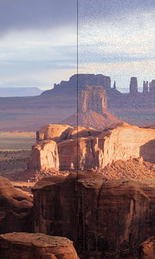
Noise appearanceThe appearance of noise is illustrated in the stepchart images on the right. Noise is usually measured as an RMS (root mean square) voltage. The mathematics of noise is presented in a green box at the bottom of this page. The patches in columns (A)-(C) are simulated. They are assumed to have a minimum density of 0.05 and density steps of 0.1, identical to the Kodak Q-13 and Q-14. They have been encoded with gamma = 1/2.2 for optimum viewing at gamma = 2.2 (the Windows/Internet standard). Strong noise— more than you’d find in most digital cameras— has been added to columns (A) and (B). Column (C) is noiseless. The fourth column (D) contains an actual Q-13 stepchart image taken with the Canon EOS-10D at ISO 1600: a very ISO high speed. Noise is visible, but low for such a high ISO speed (thanks, no doubt, to software noise reduction). The noise in (A) is constant inside the sensor, i.e., before gamma encoding. When it is encoded with gamma = 1/2.2, contrast, and hence noise, is boosted in dark areas and reduced in light areas. The On Semiconductor publication, CCD Image Sensor Noise Sources, indicates that this is not a realistic case. Shot (photon) noise causes sensor noise to increase with brightness. The noise in (B) is uniform in the image file, i.e., its value measured in pixels is constant. This noise must therefore increase with brightness inside the sensor (prior to gamma encoding), and hence is closer to real sensor behaviour than (A). Noise appears relatively constant except for the darkest zones, where it’s not clearly visible. Noise is often lower in the lightest zones, where a tonal response “S” curve superimposed on the gamma curve (or saturation) reduces contrast, hence noise. For this reason the middle zones— where noise is most visible— are used to calculate the average noise: a single number used to characterize overall noise performance. We omit zones where the density of the original chart (hence display density in an unmanipulated image) is greater than 1.5 or less than 0.1. Characteristic Stepchart results are shown below. |
|


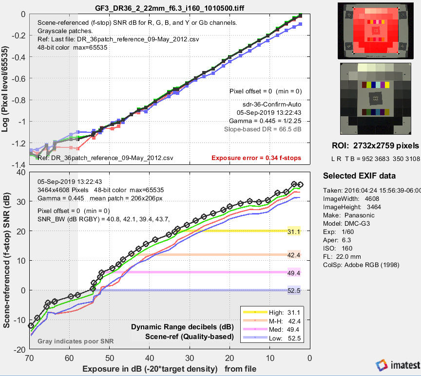
Column (D): Canon EOS-10D at ISO 1600The upper plot shows the tonal response with a slight “S” curve superimposed on the gamma curve (which would be a straight line in this log-log plot). The middle plot shows f-stop (scene-referenced) noise (the inverse of scene-referenced SNR). Dynamic range is shown for several quality levels (scene-referenced SNR = 20, 12, 6, and 0 dB). The lower plot shows the normalized pixel noise. It increases in the dark regions due to a combination of gamma-encoding and the high ISO speed. Digital cameras achieve high ISO speed by amplifying the sensor output, which boosts noise, particularly in dark regions. This curve looks different for the minimum ISO speed: noise values are much lower and subject to more statistical variation.
This is SNR in dB for the Canon EOS-10D at ISO 1600. SNR improves by about 6 dB for each doubling of exposure (0.301 density units); roughly 20 dB per decade (1 density unit), which is what would be expected for constant sensor noise. (At ISO 1600, signal and noise are multiplied by a factor of 16 over the baseline ISO 100 values, meaning the maximum signal is only 1/16 as large. In this range of illumination, shot noise is not prominent. This curve would be dramatically different at lower ISO speeds, where shot noise has an effect.) |
 |
Noise summary
There are two basic types of noise.
- Temporal. Noise which varies randomly each time an image is captured. Measured by Color/Tone Interactive, Color/Tone Auto, Colorcheck, and Stepchart using two identical input images for all modules or multiple images (4-16 with 8 recommended) for Color/Tone Interactive and Color/Tone Auto, as described in Measuring Temporal Noise.
- Spatial or fixed pattern. Noise caused by sensor nonuniformities. Sensor designers have greatly reduced fixed pattern noise in the last decade.
Temporal noise can be reduced by signal averaging, which involves summing N images, then dividing by N. This is an option for all Imatest analysis modules when several image files are selected (you can also analyze the individual files separately). Summing N individual images increases the summed signal pixel level (voltage) by N. But since temporal noise is uncorrelated, noise power (rather than voltage or pixel level) is summed. Since voltage is proportional to \(\sqrt{\text{power}}\), the noise pixel level (which is proportional to noise voltage) increases by \(\sqrt{N}\). Signal-to-noise ratio (S/N or SNR) improves by \(N / \sqrt{N} = \sqrt{N}\). S/N is improved by a factor of 2 (6.01 dB) for 4 images, 4 for 16 images, etc.
Several factors affect noise.
- Pixel size. Simply put, the larger the pixel, the more photons reach it, and hence the better the signal-to-noise ratio (SNR) for a given exposure. The number of electrons generated by the photons and the full-well (electron) capacity is proportional to the sensor area (as well as the quantum efficiency). Noise power is also proportional to the sensor area, but noise voltage is proportional to the square root of power and hence √area.
- Sensor technology and manufacturing. For a given pixel size, backside-illuminated (BSI) sensors have superior noise and SNR peroperties. We observed an improvement when we compared cameras in Shannon Information Capacity. An older technology issue was CMOS vs. CCD. Until 2000 CMOS was regarded as having worse noise, but it has improved to the point where it almost completely dominates the industry. Other aspects of sensor design and manufacturing are gradually improving with time.
- ISO speed (Exposure Index) setting. Digital cameras control ISO speed by amplifying the signal (along with the noise) at the pixel output. The higher the ISO speed, the shorter the exposure (fewer electrons reach the sensor), and hence the worse the SNR. To fully characterize a sensor it should be tested at the lowest available ISO speed. For practical applications, performance at high ISO speeds is also of interest.
- Exposure time. Long exposures with dim light tend to be noisier than short exposures with bright light, i.e., reciprocity doesn’t work perfectly for noise. To fully characterize a sensor it should be tested at long exposure times (several seconds, at least).
- Digital processing. Sensors typically have ~12-bit analog-to-digital (A-to-D) converters. When an image is converted to an 8-bit (24-bit color) JPEG, noise increases slightly. The noise increase can be worse (“banding” can appear) if extensive image manipulation (dodging and burning) is required. Hence it is often best to convert to 16-bit (48-bit color) files. Output file bit depth makes little difference in the measured noise of unmanipulated files.
- Raw conversion. In-camera raw converters, used to create camera JPEG files, usually apply noise reduction (lowpass filtering) in smooth areas and sharpening near edges whether you want it or not; even if NR and sharpening are turned off. This affects noise measurements, making it difficult to measure the sensor’s true performance. Raw converters built into Imatest (LibRaw for commercial files, Read Raw for binary files, or the Matlab demosaic function for special cases (Rawview)) minimally process images. Output from these converters is OK for noise measurements.
General comments
- Imatest subtracts gradual pixel level variations from the image before calculating noise (the standard deviation of pixel levels in the region under test). This removes errors that could be caused by uneven lighting. Nevertheless, you should take care to illuminate the target as evenly as possible.
- The target used for noise measurements should be smooth and uniform– grain (in film targets) or surface roughness (in reflective targets) should not be mistaken for sensor noise. Appropriate lighting (using more than one lamp) can minimize the effects of surface roughness.
Temporal noise
Four Imatest modules— Color/Tone Interactive, Color/Tone Auto, Colorcheck, and Stepchart— can measure temporal noise— noise that varies independently from image to image, with fixed-pattern noise omitted. It can be calculated by two methods:
- the difference between two identical test chart images (the Imatest recommended method), and
- the ISO 15739-based method, which where it is calculated from the pixel difference between the average of N identical images (N ≥ 8) and each individual image (Color/Tone Interactive and Color/Tone Auto-only).
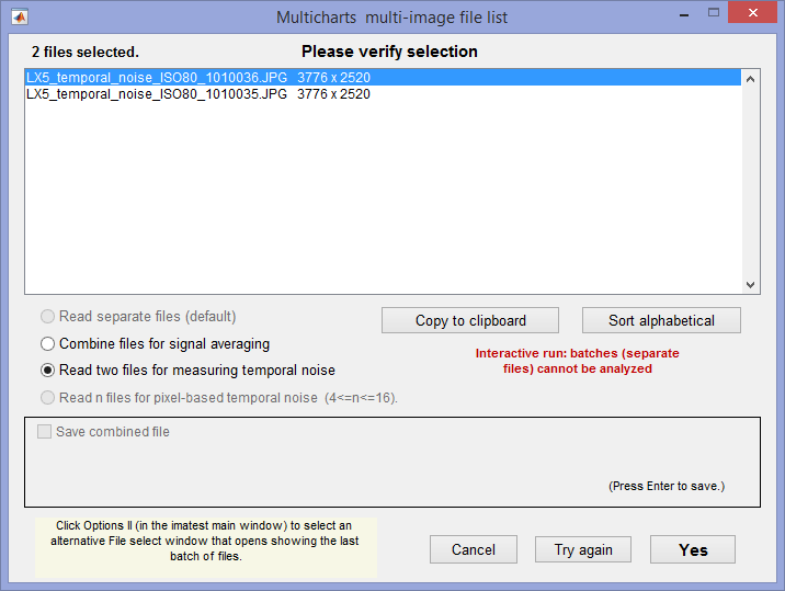
(1) Difference method. In any of the modules, read two images. The window shown on the right appears. Select the Read two files for measuring temporal noise radio button.
The two files will be read and their difference (which cancels fixed pattern noise) is taken. Since these images are independent, noise powers add. For indendent images I1 and I2, temporal noise is
\(\displaystyle \sigma_{temporal} = \frac{\sigma(I_1 – I_2)}{\sqrt{2}}\)
In Color/Tone Interactive and Color/Tone Auto, temporal noise is displayed as dotted lines in Noise analysis plots 1-3 (simple noise, S/N, and SNR (dB)).
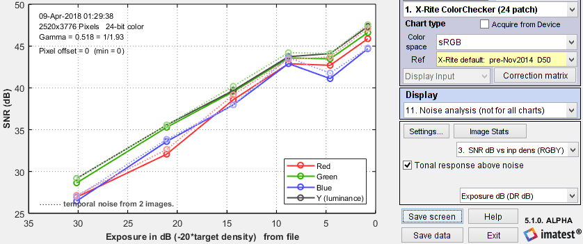 SNR (dB) for Colorchecker chart: temporal noise shown as thin dotted lines.
(2) Multiple file method. From ISO 15739, sections 6.2.4, and 6.2.5. Currently we are using simple noise (not yet scene-referred noise). Select between 4 and 16 files. In the multi-image file list window (shown above) select Read n files for temporal noise. Temporal noise is calculated for each pixel j using
\(\displaystyle \sigma_{diff}(j) = \sqrt{\frac{1}{N} \sum_{i=1}^N (X_{j,i} – X_{AVG,j})^2} = \sqrt{\frac{1}{N} \sum_{i=1}^N X_{j,i}^2 – \left(\frac{1}{N} \sum_{i=1}^N X_{j,i}\right)^2 } \)
The latter expression is used in the actual calculation since only two arrays, \(\sum X_{j,i} \text{ and } \sum X_{j,i}^2 \), need to be saved. Since N is a relatively small number (between 4 and 16, with 8 recommended), it must be corrected using formulas from Identities and mathematical properties in the Wikipedia standard deviation page. \(s(X) = \sqrt{\frac{N}{N-1}} \sqrt{E[(X – E(X))^2]}\).
\(\sigma_{temporal} = \sigma_{diff} \sqrt{\frac{N}{N-1}}\)
We currently recommend the difference method (1) because our experience so far has shown no advantage to method (2), which requires many more images (N ≥ 8 recommended), but allows fixed pattern noise to be calculated at the same time. There is a detailed comparison of the methods in Measuring Temporal Noise.
Measuring noise in raw versus demosaiced images
A customer recently questioned whether is was appropriate to measure noise in demosaiced images, where the signal in each color channel (R, G, B) is influenced by data in each of the raw color channels (R, Gr, B, and Gb). The quick answer is yes. We recommend measuring noise and SNR in the image (raw or demosaiced) that most closely resembles the use case. Raw images are best when measuring sensor performance, but demosaiced images are fine in most cases. This excellent question led us into a deep dive, which you can see by clicking the button below.
Noise frequency spectrum
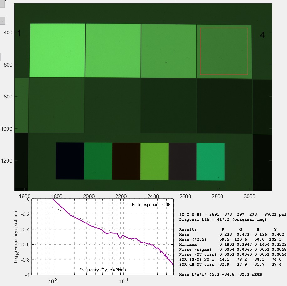
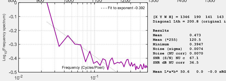
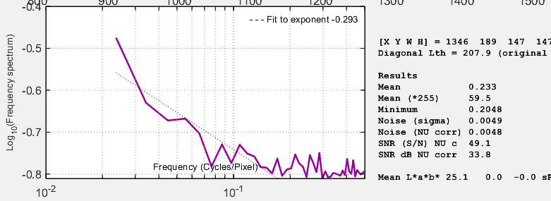
In addition to an amplitude distribution, noise is characterized by a frequency spectrum, calculated by taking the Fourier transform of the spatial image. The spectrum is closely related to appearance. Two spectra are shown below. The first is for the image from column (B), above, which contains simulated white noise. The second is for the image in column (D), above, taken with the Canon EOS-10D at ISO 1600. The images shown below have been magnified 2X (using the nearest neighbor resizing algorithm) to emphasize the pixel distribution. They are approximations to the images used to calculate the spectra (though not the exact images).
|
|
 |
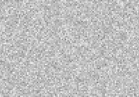 White noise, enlarged 2X (nearest neighbor) |
 Blurred noise, enlarged 2X (nearest neighbor) |
White noise (unfiltered electronic noise is white) has two key properties. 1. The values of neighboring pixels are uncorrelated, i.e., independent of one-another. 2. Its spectrum is flat. The white noise spectrum (above, left) shows statistical variation and a small peak at 0.25 cycles/pixel, probably caused when the image in column (B) was resized for display. For spectral (non-white) noise, neighboring pixels are correlated and the spectrum is not flat. The spectrum and image (above, right) are the result of blurring (also called smoothing or lowpass filtering), which can result from two causes
- The Bayer sensor demosaicing algorithm in the RAW converter causes the noise spectrum to drop by about half at the Nyquist frequency (0.5 cycles/pixel), and
- Noise reduction (NR) software lowpass filters noise, i.e., reduces high frequency components. With the widely-used bilateral filter (which can be simulated with the Image Processing module), NR uses a threshold that prevents portions of the image near contrast boundaries from blurring.
But NR comes at a price: detail with low contrast and high spatial frequencies (texture) can be lost. This causes the “plasticy” appearance sometimes visible on skin. Some people love it (plastic surgeons make a lot of income); I don’t This loss can be quantified with Imatest Log F-Contrast measurements.The visibility of noise depends on the noise spectrum, though the exact relationship is complex. Noise at high spatial frequencies may be invisible in small prints (low magnifications) but very damaging in large prints (large magnifications). Because of the complex nature of the relationship, Kodak established a subjective measurement of grain (i.e., noise) called Print Grain Index (Kodak Technical Publication E-58). Visual noise measurements are intended to predict the visual effect of noise, based on noise spectrum and viewing conditions.
Sharpening and unsharp masking (USM) are the inverse of blurring. They boost portions of the spectrum and cause neighboring pixels to become negatively correlated, i.e., they exaggerate the differences between pixels, making the image appear noisier. USM can be applied with a threshold that restricts sharpening to the vicinity of contrast boundaries. This prevents noise from degrading the appearance of smooth areas like skies. In images taken with poor quality lenses (or misfocused or shaken), the image is lowpass filtered (blurred) but the noise is not. Some sharpness loss can be recovered with sharpening or USM, but noise is boosted in the process. That’s why good lenses are important, even with digital sharpening.
ISO 15739 noise and SNR
The updated ISO 15739:2013 standard has several definitions for noise, SNR, and Dynamic Range that are similar to f-stop noise, but with some important differences. The ISO definition of Signal-to-Noise Ratio (§6.2.3-6.2.5 and Annex D) is
\( SNR = Q = gL / \sigma\)
where σ = noise in pixels, L = luminance (linear), and g is the first derivative of the OECF (pixel level vs. luminance curve).
\( g = d(\text{pixel}) / dL\) Though it isn’t obvious from the standard, L must be scaled (multiplied) by Lref, as defined in §6.2.2. The numeric version this equation is given in Annex D.
When ISO 15739 SNR is displayed in Color/Tone Interactive, Color/Tone Auto, or eSFR ISO, it can be compared with the older Imatest f-stop-based (scene-referenced) noise calculation. Results are similar (though not identical).
| (Obsolete section: kept for reference) Definitions: Pxl = pixel level (same as OL = output level in the ISO standard.) σpx = noise in pixels (note: standard deviation σ is equivalent to RMS noise.) L = Illumination or exposure level. (Units will not be important.) f-stops = log2L f-stop noise = σfst = σpx /(d(Pxl)/d(f-stops)) = σpx /(d(Pxl)/d(log2L)) f-stop SNR = SNRfst = 1/σfst = (d(Pxl)/d(log2L)) / σpx We will apply the equation, d(logb(x))/dx = 1/(x ln(b)), where ln(2) = 0.6931 = 1/1.4427. Now, from the ISO standard, Incremental gain = gI = d(Pxl)/dL (Note linear units) = d(Pxl)/d(log2L) × d(log2L) / dL = 1.442(d(Pxl)/d(log2L)) / L Appendix D of the ISO 15739 standard defines total Signal-to-Noise Ratio as SNRISO = L gI / σpx = 1.4427 L (d(Pxl)/d(log2L)) / (L σpx) = 1.4427 (d(Pxl)/d(log2L))/σpx which leads to SNRISO = 1.4427 SNRfst SNRISO is larger than SNRfst by a factor of 1.4427, or equivalently, 3.18 dB. |
Appendix I: Scene-referenced SNR and Dynamic Range
This material is in an Appendix because scene-referenced noise is used for Dynamic Range calculations, and hence is slightly outside the main topic of this page. It is repeated in
Scene-referenced noise and SNR
|
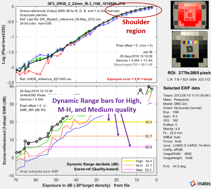
The problem — Dynamic Range (DR) is defined as the range of exposure, i.e., scene (object) brightness, over which a camera responds with good contrast and good Signal-to-Noise Ratio (SNR). The basic problem is that the camera cannot directly measure scene brightness noise, which is used to calculate scene SNR. Scene-referenced SNR must be derived from measurable quantities (the signal S, typically measured in pixel levels (equivalent to Digital Numbers, DN), and noise, which we call \(N_{DN}\)). The math — In most interchangeable image files, the signal S (typically in units of DN) is not linearly related to the scene (or object) luminance, Lscene. S is a function of Lscene, i.e., \(\displaystyle S = f_{encoding}(L_{scene})\) Interchangeable image files are designed to be displayed by applying a gamma curve to S. \(\displaystyle L_{display} = k\ S^{(display\ gamma)}\) where display gamma is frequently 2.2. For the widely used sRGB color space, gamma deviates slightly from 2.2. Although fencoding sometimes approximates \(L^{(1/display\ gamma)}\), it is typically more complex, with a “shoulder” region (a region of reduced slope) in the highlights to help improve pictorial quality by minimizing highlight “burnout”. Now suppose a perturbation \(\Delta L_{scene}\) is applied to the scene luminance, Lscene, i.e., noise Nscene. The change in signal S, ΔS, caused by this noise is \(\displaystyle \Delta S = \Delta L_{scene} \times \frac{dS}{dL_{scene} } = \ \text{pixel level (DN) noise} = N_{DN} = N_{scene} \times \frac{dS}{dL_{scene} }\) The standard Signal-to-Noise Ratio (SNR) for signal S, corresponding to Lscene is \(\displaystyle SNR_{standard} = \frac{S}{\Delta S} = \frac{S}{N_{DN}} \) SNRstandard is often a poor representation of scene appearance because it is strongly affected by the slope of S with respect to Lscene ( \(dS/dL_{scene}\)), which is often not constant over the range of L. For example, the slope is reduced in the “shoulder” region, and it can also be reduced by stray light in dark regions. A low value of the slope will result in a high value of SNRstandard that doesn’t represent the scene. To remedy this situation we define a scene-referenced noise, Nscene-ref , that has the same units (DN) as signal S, and gives the same SNR as the scene itself: SNRscene-ref = S/Nscene-ref = Lscene / Nscene. SNRscene-ref is a better representation of scene appearance. \(\displaystyle N_{scene-ref} = \frac{N_{DN}}{dS/dL_{scene}} \times \frac{S}{L_{scene}}\) \(\displaystyle SNR_{scene-ref} = \frac{S}{N_{scene-ref}} = \frac{L_{scene}}{N_{DN}/(dS/dL_{scene})} = \frac{L_{scene}}{N_{scene}} = SNR_{scene} \) SNRscene-ref = SNRscene is a key part of dynamic range (DR) calculations, where DR is limited by the range of illumination where SNRscene-ref is greater than a set of specified values ({10, 4, 1, 1} = {20, 12, 6, 0 dB}, which correspond to “high”, “medium-high’, “medium”, and “low” quality levels. (We have found these indications to be somewhat optimistic.) Example — \(\log_{10}(S)\) as a function of\(\text{Exposure in dB} = -20 \times \log_{10}(L_{scene}/L_{max})\)is displayed in Color/Tone and Stepchart results. (Color/Tone is generally recommended because it has more results and operates in both interactive and fixed, batch-capable modes). \(dS/dL_{scene}\) is derived from the data used to create this plot, which has to be smoothed (modestly — not aggressively) for good results. Results from the JPEG file (the camera also outputs raw) are shown because they illustrate the “shoulder” — the region of reduced slope in the highlights. |
|
The human vision perspective:
|

|
\(\displaystyle \text{F-stop noise } = N_{f-stop} = \frac{N_{DN}}{dS/d(\text{f-stop})} = \frac{N_{DN}}{dS/d(\log_2 ( L_{scene})}\) \(\displaystyle\text{Using }\ \frac{d(\log_a(x))}{dx} = \frac{1}{x \ln (a)} \ ; \ \ \ \ \ d(\log_a(x)) = \frac{dx}{x \ln(a)} \) \(\displaystyle N_{f-stop} = \frac{N_{DN}}{dS/dL_{scene} \times \ln(2) \times L_{scene}} ≅ \frac{N_{DN}}{dS/dL_{scene} \times L_{scene}} \) where Npixels is the measured noise in pixels and \(d(\text{pixel})/d(\text{f-stop})\) is the derivative of the signal (pixel level) with respect to scene luminance (exposure) measured in f-stops = log2(luminance). ln(2) = 0.6931 has been dropped to maintain backwards compatibility with older Imatest calculations. Noting that luminance (exposure) is the signal level of the scene, \(\displaystyle \text{Scene noise} = N_{scene} = \frac{N_{DN}}{dS/dL_{scene}} ≅ N_{f-stop} \times L_{scene} \) The key to these calculations is that the scene-referenced Signal-to-Noise Ratio, calculated from the measured signal S and noise Npixels must be the same as the scene SNR, which is based on Nscene, which cannot be measured directly. \(\displaystyle \text{Scene Signal-to-Noise Ratio} = SNR_{scene} = \frac{L_{scene}}{N_{scene}} = \frac{1}{N_{f-stop}} = \text{Scene-referenced SNR} = SNR_{scene-ref} \) the equation for Scene-referenced noise, \(N_{scene-ref}\), which enables \(SNR_{scene-ref} = SNR_{scene}\) to be calculated directly from \(S/N_{DN}\) is given above. Displays in Stepchart, Color/Tone Interactive, and Color/Tone Auto offer a choice between f-stop noise or Scene-referenced SNR (expressed as a ratio or in dB). Note that SNRscene-ref decreases as the slope of the tonal response curve decreases (often the result of flare light in dark patches). |
The above-right image illustrates how the pixel spacing between f-stops (and hence d(pixel)/d(f-stop)) decreases with decreasing brightness. This causes f-stop noise to increase with decreasing brightness, visible in the figures above.
Imatest has several types of Dynamic Range calculation, which are cross-referenced here.
| Dynamic range from a single transmissive chart image. | Stepchart, Color/Tone Interactive, Mutitest | A transmissive chart is such as the Imatest 36-patch Dynamic Range or HDR chart is required because reflective charts do not have sufficient tonal range. |
| Dynamic range from multiple (differently exposed) images | Dynamic Range module | Uses CSV output of Stepchart of Color/Tone Auto for several differently exposed images. Usually used with reflective charts, but transmissive charts may also be used. |
| ISO 15739 Dynamic Range from patch with density ≈ 2 | Color/Tone Interactive, Color/Tone Auto, eSFR ISO | Extrapolates Dynamic Range from a single patch with density ≈ 2. |
| Raw sensor Dynamic Range | Color/Tone Interactive, Color/Tone Auto | Fits raw data to an equation from the EMVA 1288 standard, then extrapolates to find DR. The test chart does not have to have as large a tonal range as the DR, but transmissive charts with tonal range ≥ 3 are recommended. |
Since scene-referenced noise and SNR are independent of the tonal response curve, they are used as the basis for Imatest Dynamic Range calculations, which are described elsewhere. Dynamic Range is the range of exposure (scene brightness) where quality exceeds a specified level, which we define as 20 dB for “high quality” down to 0 dB for “low quality”. Here is an illustration. The upper curve is the tonal response plot showing gamma. The lower plot is the scene-referenced noise, showing Dynamic Range at several quality levels.
 Tonal response and scene-referenced SNR for an image converted from raw with LibRaw.
Appendix II: The mathematics of noise (just a taste)
|
Amplitude distribution
|
 In most cases, the pixel or density variations that comprise noise can be modeled by the
 Links
CCD Image Sensor Noise Sources (from On Semiconductor) An excellent, highly readable introduction to the different noise sources. Noise sources in CMOS sensors differ only in relative magnitude.
Neat Image is a remarkable program for reducing noise. Instead of lowpass filtering, the software is trained to recognize the structure of the noise. It can reduce noise with minimal side-effects. Particularly valuable at high ISO speeds.
EMVA 1288 Standard contains an excellent, well-written introduction to the mathematics of noise.
Photography — Electronic still-picture imaging — Noise measurements (ISO 15739:2003) Somewhat difficult to read, but it’s the official standard. Its Dynamic Range measurement is extrapolated from measurements from a black reference density of 2.0.