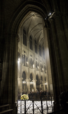
Image of an HDR scene with local tone mapping
Dynamic Range (DR) is the range of exposure, i.e., scene brightness, over which a camera responds with good contrast and good Signal-to-Noise Ratio (SNR). This is a scene-dependent image quality factor that incorporates sensor sensitivity, noise, and stray light.
High Dynamic Range (HDR) scenes have a ratio between light and dark areas that exceeds 10,000:1 (80dB; 4.0 Optical Density; 13.3 f-stops). See below for how to achieve HDR imaging. Some examples of HDR Scenes:
- Mixed indoor/outdoor scene. Entering or exiting a tunnel or parking garage, A door or window open to the brightly lit outdoors, a shadowed area cast by an opaque object in direct sunlight.
- Bright lights in dark scenes. The sun in a daytime scene, headlights or streetlights in a nighttime scene. The bright moon on the dark sky
Local Tone Mapping (LTM) – Often, high dynamic range images need to be converted to low dynamic range images to be presented on low dynamic range prints or displays. LTM is a nonlinear process of increasing local contrast in different image regions to present high-contrast details across a wide range of scene luminance levels. LTM can result in a loss of mid-tones, and can invalidate conventional measurement techniques.
Achieving HDR – Sensor vs. System DR – Flare, Charts, Exposure – DR definitions – Transmission chart –
Lightbox – How to measure DR – Overexposure – Minimizing reflections –
Contrast Resolution chart – Information-based Dynamic Range (InfoDR) –
Tips and recommendations – Tone mapping – Offsets –
More on Flare – Flare light-limited DR – F-stop noise & scene-referenced SNR –
See Also:
- Dynamic Range Details
- Stray Light (flare) – a factor which limits dynamic rage
- Contrast Resolution – A special transmissive chart for measuring the visibility of low contrast features in larger fields over a wide dynamic range
- Making Dynamic Range Measurements Robust Against Flare Light
Related Standards:
Dynamic Range Details
|
Dynamic Range Measurement tips The environment should be completely darkened. Take great care to avoid stray light and reflections. Frame the chart so it occupies the central portion of the image (for most medium-high resolution cameras). Enter a reference file to obtain valid results with transmissive Dynamic Range charts. Remove pixel offset (pedestal) if present. Beware tone-mapped images, often recognizable by very low gamma (<0.25). They can seriously throw off DR measurements with standard grayscale charts. The Contrast Resolution chart is recommended. |
Achieving HDR (High Dynamic Range)
HDR Imaging can be achieved by a combination of various factors:
- HDR sensing techniques
- High-sensitivity image sensors: Larger pixels and increased sensor quantum efficiency and low dark noise enables more light to be captured. This approach limits resolution.
- Multi-exposure combination: Several exposures are performed: shorter exposures for bright scene content and longer exposures for dark scene content. This time division does not support the motion of the scene or the camera.
- Split pixel sensors: Rather than temporal division of exposure length, shorter exposures are achieved by mixing smaller (bright light) pixels with larger (low light) pixels. This approach can cause mosaic color artifacts on the edges of the image.
- High-Quality optical components: anti-reflective coatings on lens elements, lens barel and camera body. Baffeling to reduce stray light.
- HDR Image encoding
- High bit depth (>= 16bits)
- Companding to make the available bits span a larger range of luminance levels. A medium-bit depth commanded image can be expanded into a high-bit depth linear image.
- Media Formats – such as HDR10, Dolby Vision, HLG
- Display / print technology
- HDR Displays – able to produce deep blacks as well as and bright regions, potentially utilizing techniques such as ISO 21496 Gain Map
- HDR Transparencies – For HDR prints including test targets, a back lit transparent that is capable of is necessary
Sensor vs. System Dynamic Range
Sensor manufacturers are developing High Dynamic Range (HDR) image sensors that claim exceptional dynamic ranges: 120dB to as much as 150dB. Measured system (camera) dynamic range is typically much lower than the specified sensor dynamic range.
The primary cause is flare light in the lens— stray light reflected between lens elements and off the barrel (on the interior of the lens) that fogs the image and sometimes causes “ghost” images. High quality lens coatings help— but only so much. Different test chart designs have different density distributions, and hence have different amounts of lens flare on the chart image— leading to differences in measured dynamic range. This is why standardization is important. No camera system we know of (where light has to pass through optics) reaches 120 dB. (100dB is about the best we’ve heard of (summer 2017).)
Flare light, test chart design, exposure, and Dynamic Range measurements
As a result of the three factors (especially flare light), test chart standardization is extremely important. (If there were no flare light, all test charts would have similar DR measurements.) It might be necessary to specify more than one standard chart: one with a gray background (that should work with autoexposure) and others with dark backgrounds or smaller bright patches. |
Sensor dynamic range (the range of brightness between sensor saturation and SNR = 1 (0 dB)) can be measured for linear (not HDR) sensors from absolutely raw images (no demosaicing or processing of any kind) with Color/Tone Interactive or Color/Tone Auto (formerly Multicharts and Multitest) using a technique described in Color/Tone/eSFR ISO Noise. It can also be measured with a sequence of flat field exposures (often involving calibrated neutral density filters), as described in the EMVA 1288 standard. These measurements should not be confused with a camera or system measurements (especially for HDR systems) because the images used for the measurement has zero dynamic range, and hence don’t correspond to scenes in real cameras.
ISO 15739: The dynamic range corresponding Scene-referenced Signal-to-Noise Ratio SNRscene = 1 (0dB) corresponds to the intent of the ISO 15739 Dynamic range definition in section 6.3 of the ISO noise measurement standard: ISO 15739: Photography — Electronic still-picture imaging — Noise measurements. Imatest Dynamic Range differs in several details from ISO 15739 (though we do measure ISO 15739 Dynamic Range); hence the results are not identical. Imatest produces more accurate results because it measures DR directly from a transmission chart, rather than extrapolating results for a reflective chart with maximum density = 2.0.
| Measurement | Modules | Description |
| Dynamic range from a single transmissive chart image. | Stepchart, Color/Tone Interactive & Auto | A transmissive chart is such as the Imatest 36-patch Dynamic Range or HDR chart is required because reflective charts do not have sufficient tonal range. |
| Dynamic range from multiple (differently exposed) images | Dynamic Range (postprocessor) module | Uses CSV output of Multitest or Stepchart from several differently-exposed images. Usually used with reflective charts, but transmissive charts may also be used. No longer recommended because, especially for HDR situations, because flare light has an unrealistically small effect on the individual reflective images. |
| ISO 15739 Dynamic Range from patch with density ≈ 2 | Color/Tone Interactive & Auto, eSFR ISO |
Extrapolated Dynamic Range from a single patch with density ≈ 2. |
| Raw sensor Dynamic Range | Color/Tone Interactive & Auto | Fits raw data to an equation from the EMVA 1288 standard, then extrapolates to find DR. The test chart does not have to have as large a tonal range as the DR, but transmissive charts with tonal range ≥ 3 are recommended. Only for linear (non-HDR) sensors. |
| Contrast Resolution | Color/Tone Interactive & Auto | Measures the visibility of low contrast features over a wide tonal range. A better indication of true usable DR than traditional measurements. Not yet an industry standard (as of Sept. 2017), but we’re working on it. |
| Module | Brief description and recommendations | |
| Color/Tone Interactive (Multicharts) | Interactive module for measuring color and grayscale charts. Best when you need to closely examine the results. | Supports several measurements not in Stepchart, including ISO noise, sensor dynamic range, and Contrast Resolution. Color/Tone Interactive and Auto share most INI file settings. They include all Stepchart capabilities. |
| Color/Tone Auto (Multitest) | Fixed (batch-capable) module for measuring color and grayscale charts. Same functions and INI file settings as Color/Tone Interactive. Largely replaces Colorcheck and Stepchart (older modules with limited capabilities). | |
| Stepchart | Older (legacy) module for measuring grayscale step charts (named after the Kodak Q13/Q14 charts). | |
|
Quality (SNR)-based Information-based is a good choice for new work. |
the range of exposure where
SNR tends to be worst in the darkest regions. |
SNRscene ≥ 10 = 20dB; high quality SNRscene ≥ 4 = 12dB medium-high quality SNRscene ≥ 2 = 6dB; medium quality SNRscene ≥ 1 = 0dB; low quality |
| Information-based |
Introduced in Imatest 26.2, April 2026. Based on C4 information capacity (the amount of information an object with 4:1 contrast ratio can convey). Uses the new InfoDR test chart. Should correlate better with performance than SNR-based DR. |
|
|
Slope-based (Not recommended by itself, but used in Imatest 5.2+ to limit quality-based DR) |
The range of exposure where slope of the density curve is greater than 7.5% of the maximum slope (on the dark side) and less than 98% of the saturation level (on the light side). Must be measured with care since noise and irregular density steps in the original data affect patch levels, and hence slope measurement. Test chart density is interpolated to have 101 evenly-spaced points, then the log Digital Number for these points is found using the Matlab interp1 function. The curve is smoothed using a rectangular kernel 7 points wide (approximately 1/14 of the total range). This algorithm gives better results than earlier (pre-4.4) Patch range and detected DR measurements. Slope-based Dynamic Range it is NOT recommended because SNR can be extremely low (often well under 1 = 0 dB) in the the dark portion of the range, resulting in measurement inconsistencies as well as overly optimistic measurements, since the image is meaningless (it’s all noise) when SNR < 1. Slope-based DR can be falsely increased by tone mapping and by medium-range flare light (bleeding from light chart patches, visible in the Image Statistics images below). The Contrast Resolution chart and analysis provides a much better indication of true camera (system) DR. |
|
Transmissive step charts
The most straightforward way to measure a camera’s (or scanner’s) dynamic range is with a transmissive step chart illuminated from behind by a lightbox (taking care to minimize light reaching the front of the chart). Reflective step charts such as the Kodak/Tiffen Q-13 or Q-14 are inadequate because their density range of around 1.9 is equivalent to 1.9 * 3.32 = 6.3 f-stops (38 dB), well below that of digital cameras (although they can be used to obtain an approximate DR measurement from several different exposures combined in the Dynamic Range postprocessor for Multitest and Stepchart: this approach is not recommended because it neglects flare light).
The table below lists several transmission step charts, all of which have a density range of at least 3 (10 f-stops). Several of the charts are linear (one row of patches), and may suffer from vignetting (light falloff) as a result. All except the Imatest charts have dark backgrounds, which makes is difficult to achieve correct exposure in autoexposure systems.
| Product | Steps | Target density or density increment: Note that density = log10(incident light / transmitted light). |
Dmax | Size |
| Reference files should always be used when analyzing 36-patch Dynamic Range charts (below) because the target densities (the input to the manufacturing process for photographic film) cannot be achieved exactly. Reference files help with irregular density steps. When the reference file is entered into Imatest, results will be accurate and reliable. |
||||
| Imatest 36-patch ITDR36 Dynamic Range test chart | 36 | ~0.10 (1/3 f-stop); Reference file required Target (not actual) densities: 0.00 0.10 0.20 0.30 0.40 0.50 0.60 0.70 0.80 0.90 1.00 1.10 1.20 1.30 1.40 1.50 1.60 1.70 1.80 1.90 2.00 2.10 2.20 2.30 2.40 2.50 2.60 2.70 2.80 2.90 3.00 3.10 3.20 3.30 3.40 3.50 | >2.8 | 8×10″ |
| Imatest 36-patch ITWDR36 Wide Dynamic Range test chart (recommended) | 36 | ~0.10 – 0.30 (1/3 – 1 f-stop); Reference file required Target (not actual) densities: 0.15 0..29 0.42 0.56 0.69 0.83 0.96 1.10 1.24 1.37 1.51 1.64 1.78 1.91 2.05 2.19 2.32 2.46 2.59 2.73 2.86 3.00 3.21 3.43 3.43 3.64 3.86 4.07 4.29 4.50 4.71 4.93 5.14 5.36 5.57 5.79 6.00 | >5 | 8×10″ |
| Imatest 36-patch ITUHDR36 Ultra High Dynamic Range test chart | 36 | ” ” Target (not actual) densities: 0.00 0.10 0.20 0.30 0.40 0.50 0.60 0.70 0.80 0.90 1.00 1.10 1.20 1.30 1.50 1.70 1.90 2.10 2.30 2.50 2.70 2.90 3.43 3.73 4.02 4.32 4.63 4.92 5.23 5.52 5.82 6.27 6.72 7.17 7.63 8.22 |
>7.5 | 8×10″ |
| Imatest InfoDR Information-based Dynamic Range chart |
42 |
Patch densities: 0 to 5.2 in steps of 0.2 (104 dB). 42 total, 27 distinct levels; |
5.2 (4.6) |
8×10″ (more planned) |
| Imatest Contrast Resolution chart | 20 | 0.25 (with 2:1 inner patches) | 4.75 | 8×10″ |
| ISO 21550 | 24 | Use General m x n chart with Rows (m) = 4 and Columns (n) = 6. On 35mm film. Reference file: ISO-21550_0-4_reference |
4.03 | 0.8×1.2″ 20×30 mm |
| Kodak Photographic Step Tablet No. 2 or 3. Calibrated or uncalibrated (usually sufficient). |
21 | 0.15 (1/2 f-stop) Linear pattern* | 3.05 | 1x5.5″ (#2) larger (#3) |
| Stouffer Transmission Step Wedge T4110 | 41 | 0.10 (1/3 f-stop) Linear pattern* | 4.05 | 1x9″ |
| Danes-Picta TS30D (Digital Imaging page) | 28 | 0.15 (1/2 f-stop) Linear pattern* | 4.2 | (0.4x9″) |
| DSC Labs Xyla 15, 21, and 26 step HDR Greyscale | ≥13 | 0.30 ( 1 f-stop) Linear pattern* | 3.7 | (large) |
| Image Engineering TE269 (36 patches) (You can choose between old TE269 and the new TE269V2 in the ROI options window.) |
36 |
The TE269, which has a similar geometry to the Imatest 36-patch charts but a different patch order, is fully supported by Imatest. Three standard reference files are available, derived from data on the manufacturer’s website: TE269A | TE269B | TE269C The 20-patch TE241 and TE264 charts have extremely large optical density (OD) steps between their darkest patches (19-20): 2.37 OD = 47.4dB for the 1,000,000:1 versions and 1.5 OD = 30dB for the 100,000:1 versions). For this reason, 20-patch OECF charts should not be used for Dynamic Range (and especially HDR) measurements. 36-patch charts were developed to overcome this shortcoming. |
4−6 | D280 |
| *Region selection is less robust with linear (single-row) charts because it’s difficult to locate features in very dark areas. Also, linear charts are more subject to vignetting than charts with a circular arrangement of patches. |
||||
| Most transmissive dynamic range test charts require a reference file (usually with a single density value per line, but L*a*b* values also work). Note that log(luminance) of a patch is proportional to (–)density. The only exceptions are the Stouffer T4110, the TE269, and the DSC Labs Xyla charts, which have consistent density steps. | ||||
The Imatest 36-patch Wide Dynamic Range (HDR) test chart, with target density steps from 0.1 to 0.3 (actual steps may differ; the individual reference file should always be used for Imatest analysis) and a maximum density of at least base+5 (~17 f-stops), is recommended for traditional Dynamic Range measurements. A nearly circular patch arrangement ensures that vignetting has minimal effect on results. A CSV or CGATS reference file with actual densities (required with the HDR chart) is supplied. the chart has an active area of 7.75×9.25 inches on 8×10 inch film.
It also contains slanted edges in the center and corners with 4:1 contrast for measuring MTF. Registration marks make the regions easy to select, and fully automated region detection is available in Imatest 4.0+. A neutral gray background helps ensure that the chart will be well-exposed in auto exposure cameras (compared to charts with black backgrounds, which can be strongly overexposed unless manual exposure is available).
 Imatest 36-patch Dynamic Range chart Imatest 36-patch Dynamic Range charton 8×10 film. Dmax ≈ 3. |
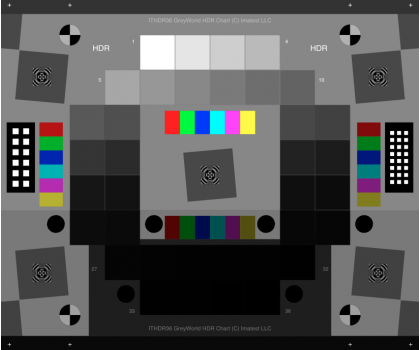 Imatest 36-patch High Dynamic Range chart Imatest 36-patch High Dynamic Range charton 8×10 film. Dmax > 5. |
This chart is produced with a high-precision LVT film recording process for the best possible density range, low noise, and fine detail.
The standard 36-patch Dynamic Range chart can be used with the Dynamic Range postprocessor to measure dynamic ranges larger than 11 f-stops if several manual exposures are available, but this approach is not recommended because the important effects of flare light are not handles properly.
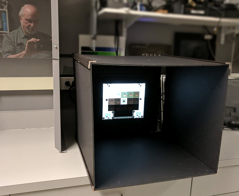
Lightbox
 You’ll need a lightbox that can evenly illuminate the transmission step chart. 9×12 inches (26×22 cm) is large enough in most cases. Avoid thin or “mini” models, which may not have even enough illumination. Fluorescent light boxes should have high-frequency ballasts to eliminate flicker.
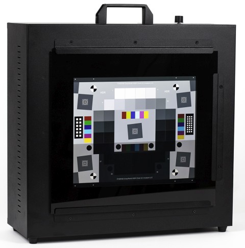
We recommend the Imatest LED Lightbox (shown on the right with the 36-patch HDR chart), available from the Imatest store. It has
- Highly uniform illumination: ~95% uniformity.
- High quality spectral response. The standard version allows you to choose between 3100K, 4100K, 5100K, 5500K, 6500K color temperature with a Color Rendering Index (CRI) of 97 and near-infrared wavelengths of 850nm and 940nm. Other color temperatures are available as options.
- Adjustable intensity via a hardware knob, WiFi, or USB from 30-10,000 lux equivalent: a range of over 300:1, making it suitable for measurements from near-daylight to extremely dim light. Versions low-light settings of 1 lux and ultra-bright settings up to 100,000 lux are available.
Several lightboxes are available from the Imatest Store. There are compared in the Lightbox Comparison Guide. The GLE-10 and GLE-16E have well-controlled color temperatures. The Imatest LED Lightbox and Light Panels are extremely reliable and have a variety of options.
How to measure Dynamic Range
| Unit | Scaling | Notes | Used by |
| f-stops | log2; Factor of two | also called zones or EV (Exposure Value); | Photographers |
| decibels (dB) | 20 log10 | 1 density unit = 20dB; one f-stop = 6.02dB | electrical engineers |
| density units | log10; Factor of ten | 1 density unit = 3.322 f-stops | optical scientists |
The lightbox and chart are shown inside a black box that minimizes stray light reflecting back to the chart. |
 |
|
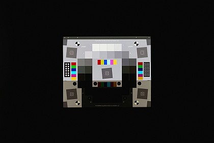 |
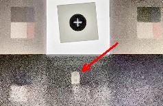
 Here is an example of an image with a framing problem. Flare light from the lightbox surrounding the chart will decrease the measured dynamic range. Avoid this unless you want to measure the effects of flare light.
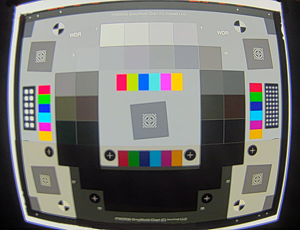
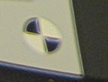 The image on the right has another problem, shown in the crop on the left. Strange signal processing (sharpening) makes the registration marks difficult to detect, so you may need to manually select the chart region (instead of using the much more convenient auto detection).
- Photograph the chart in a totally darkened room. No stray light should reach the front of the target; it will distort the results. The surroundings of the chart and camera should be kept as dark as possible to minimize flare light.
- Expose carefully, taking care to avoid overexposure, which is common in charts with dark backgrounds. An overexposed image has several (>2) clipped patches (at the maximum allowed level for the bit depth and image processing). Where possible manual exposure should be used to ensure correct exposure: no more than 1 or 2 patches should be clipped. We have seen images where half the patches are clipped: DR measurements from such images are meaningless.
-
For flatbed scanners with transparency units (light sources for transparencies), you can simply lay the step chart down on the glass. Stray light shouldn’t be an issue, though there is no harm in keeping it to a minimum. 35mm film scanners may be difficult to test since most can only scan 35mm segments. (Most transmissive targets are longer.)
- Where possible, save the image in a 16-bit (or more) format. Note that JPEG images are always 8 bits (Digital Numbers (pixel levels) 0-255). This can seriously compromise dynamic range measurements, especially for HDR cameras.
- Follow the instructions for running Color/Tone Setup (formerly Multicharts), Color/Tone Auto (formerly Multitest), or Stepchart (a legacy module not recommended for new work) for analyzing the image.
-
Be sure to select the correct chart type in the Settings window. These programs support a variety of linear (single row) and multiple row (often in a circular arrangement) charts.
|
You MUST enter a reference file to obtain valid results with 36-patch Dynamic Range charts. Individually-measured reference files are supplied with every 36-patch chart. (We can usually locate the file if you’ve lost it.) For more detail, go to Color/Tone Interactive — Reference files. Reference files are also recommended for measuring tonal response (OECF) or Dynamic Range from the Contrast Resolution chart and ALL transmissive charts. |
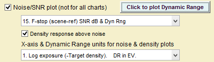 Tip: to facilitate Dynamic Range plots in Color/Tone Auto (Multitest) we’ve added a button to the settings window. Pressing it enters the correct settings for a DR display (checks the Noise/SNR plot, and selects 15. F-stop…SNR and Density response above noise). the X-axis & DR units are unaffected. Tip: to facilitate Dynamic Range plots in Color/Tone Auto (Multitest) we’ve added a button to the settings window. Pressing it enters the correct settings for a DR display (checks the Noise/SNR plot, and selects 15. F-stop…SNR and Density response above noise). the X-axis & DR units are unaffected. |
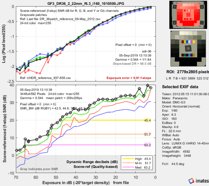
Here are Color/Tone and Stepchart results for the Panasonic G3 (a Micro Four-Thirds camera with 3.75 micron pixel pitch) at ISO 160, converted from raw using dcraw with the following settings: Demosaicing: Normal RAW conversion (demosaiced), Output gamma: 2.2, White Balance: Camera, Output color space: 48-bit, Quality: Default.
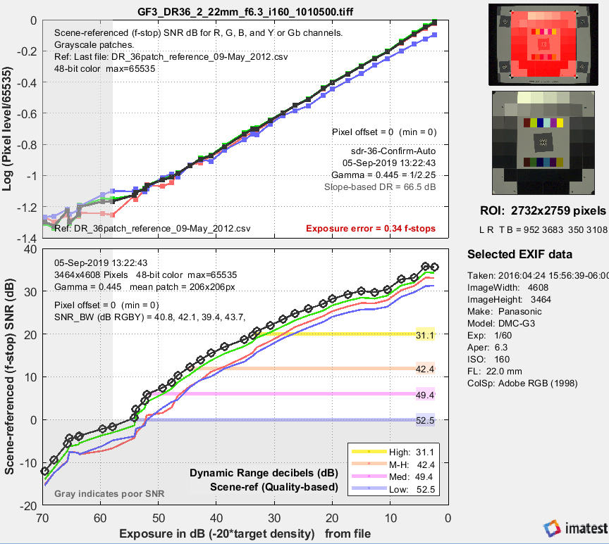 Panasonic G3, ISO 160, Converted with dcraw, run with Multitest.
The grayed-out area on the left of both plots is where the slope of log(Digital Number) vs. (log) exposure (the contrast) < 0.075 * the maximum slope. Images in this region are useless because of their extremely low contrast. The grayed-out area at the bottom of the lower plot is where the scene-referenced SNR < 0 dB (S/N < 1). Images in this region are useless because noise overwhelms the signal.
| Dynamic range legend | Line color | Quality level | S/N | SNR (dB) |
|
Dynamic Range is the range of exposure where
|
L (Low) | 1 | 0 | |
| M (Medium) | 2 | 6 | ||
| M-H (Medium-High) | 4 | 12 | ||
| H (High) | 10 | 20 |
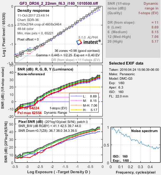 Although the slope-based dynamic range is greater than 11 f-stops (66dB), it is meaningless because it includes patches with SNR below 0 dB, where noise overwhelms visible features, i.e., no image detail is visible.
The DR at low quality level (scene-referenced SNR = 1 = 0dB) is 8.7 f-stops (52.4 dB), decreasing to 5.17 f-stops at high quality level (SNR = 10 = 20dB). These results are similar for 24-bit raw conversion.
Same Panasonic G3 image, run with Stepchart.
Click on image for full-sized display.
The shape of the response curve is a strong function of the conversion software settings. The plot below is for the same exposure, saved as a JPEG file inside the camera. Note that the transfer curve is quite different: it has a “shoulder” in the highlights, which improves pictorial quality by reducing the tendency of highlights to saturate (“burn out”). Dynamic Range is increased due to software noise reduction (absent in the dcraw conversion).
 Panasonic G3, ISO 160, in-camera JPEG, run with Color/Tone Auto. Note the “shoulder.”
Dynamic range is improved due to software noise reduction.
 In Stepchart, units for displaying Dynamic Range can be set in the X-axis scale (Figs 2-4) and Dynamic Range units (Fig. 2) dropdown menu. To convert dynamic range from f-stops into decibels (dB), the measurement normally given on sensor data sheets, multiply the dynamic range in f-stops by 6.02 (20 log10(2)). The dynamic range for low quality (f-stop noise = 1; SNR = 1) corresponds most closely to the number on the data sheets. (A valid sensor Dynamic Range measurement requires completely raw images.)
Panasonic G3, ISO 160, in-camera JPEG,
run with Stepchart. Click on image for full-sized display.
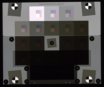
The Contrast Resolution chart
The Contrast Resolution chart was developed to overcome critical limitations of standard DR measurements derived from grayscale charts. We are working on standardizing it, especially in the IEEE P2020 standard for automotive system image quality. A paper that describes the Contrast Resolution chart, presented at Electronic Imaging 2018, can be downloaded here.
 The key to understanding the Contrast Resolution chart is that Dynamic Range can be defined more meaningfully when it predicts the visibility of low contrast features over a range of tones, i.e., answers the question, “Will a low contrast feature be visible in a dark (or light) area of the image?” Standard DR measurements don’t provide a clear, unambiguous answer to this question.
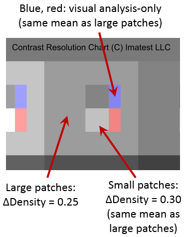
The Contrast resolution chart consists of 20 large patches that cover a 95 dB tonal range. Each large patch contains four smaller patches. The light and dark gray patches have a 2:1 (6 dB) contrast ratio (100% Weber contrast) and the same mean density as the surrounding large patch. The difference between them defines the signal for the newly-developed Contrast Resolution Signal-to-Noise Ratio (SNRCR) measurement, where the noise is measured in the larger gray patch, which has better noise statistics. This signal is not distorted by flare light, uncorrected black level offset, or tone mapping. The red and blue patches are for visual analysis only.
 Before we say more, we have to answer the question,
“Why only 95 dB when sensors have up to 150 dB dynamic range, and there is getting to be quite an intense DR competition? (This competition is somewhat akin to the automotive horsepower race of the 1950s, which culminated when TV comedians adopted the line, “My car can pass anything on the road except a gas station.”)”
The answer is we have yet to see a real practical camera whose dynamic range (which is always limited by flare light) reaches 95 dB, much less surpasses it. (Also, it’s more expensive to manufacture practical charts of this type with a higher tonal range). Customers who expect higher dynamic ranges from sensors specified at up to 150 dB DR may not be pleased by the harsh reality of placing a lens between the sensor and the test chart or scene. Please contact us at [email protected] if your camera’s DR exceeds 95 dB.
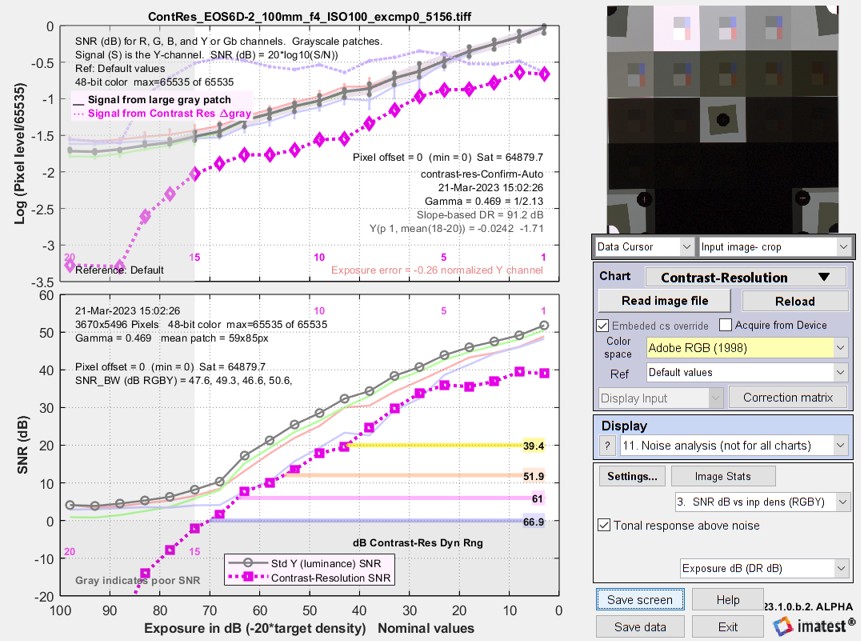
Standard (—) and Contrast Resolution (—) signal (top) and SNR (bottom). Note dB = 20*density.
Here is a brief explanation of Contrast Resolution measurements. See the Contrast Resolution page for full details.
The example on the right, run on Color/Tone Interactive, uses an image of the Contrast Resolution chart taken with the Canon EOS-6D and 100mm f/2.8 macro lens at f/4, converted to a 48-bit color file (bit depth = 16)— a very high quality DSLR camera and lens, but not specifically marketed as HDR (High Dynamic Range).
Log Digital Numbers (pixel levels) for the large gray patches, which are used as the signals in standard DR analyses, are shown in the upper plot as thin black lines. The Contrast Resolution signal (light-dark levels) is shown as thick magenta lines.
The lower plot shows standard SNR (thin black line) and Contrast Resolution SNR (SNRCR), where the signal is the small light-dark patch level and the noise is measured in the larger adjacent gray area. The colored horizontal lines are Contrast Resolution Dynamic Ranges (DRCR) corresponding to SNRCR = 20, 12, 6, and 0 dB (S/N = 10, 4, 2, 1; optimistically designated as “High”, “Medium-High”, “Medium”, and “Low” quality). The small patches are clearly distinguishable (high quality) at SNR = 20 dB, but barely distinguishable (low quality) at 0 dB.
|
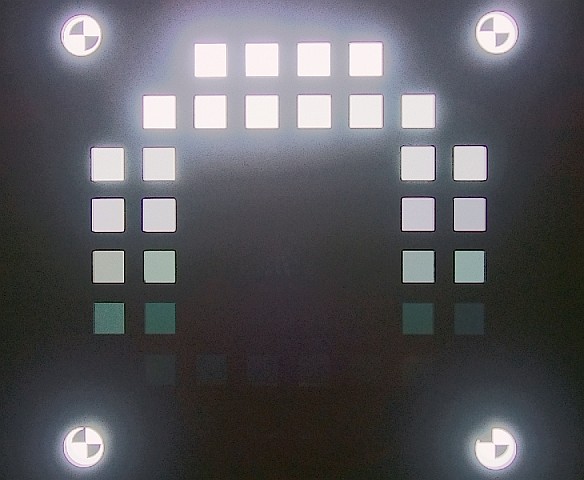
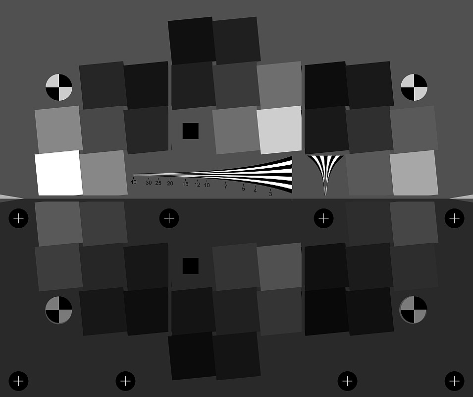
The image on the right displays all patches at a constant mean Digital Number, making it easy to visualize the effects of noise. The 2:1 (100% Weber) contrast features are clearly visible in patches 1-13, are fading badly in patches 14 and 15, and are pretty much gone beyond that. Patch 13 has about 7.7 dB (20*log10(2.43)) Contrast Resolution SNR. The definition of Contrast Resolution Dynamic Range DRCR is based on the range of tones where SNRCR is greater than the levels specified above (20, 12, 6, and 0 dB; S/N = 10, 4, 2, 1). Note that SNRCR = 1 (used to define DR in conventional measurements) corresponds to quite horrible image quality, where features are only marginally visible only if you know exactly what to expect. |
Click on the images to display them full-sized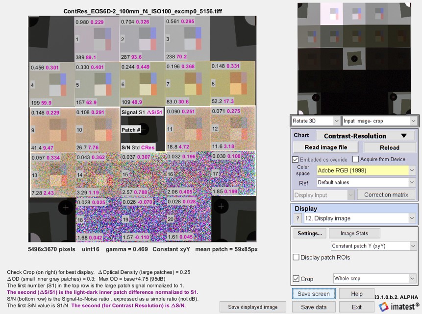 Image with patches normalized Image with patches normalizedto have the same mean pixel level. |
A key advantage of the Contrast Resolution chart is that it provides good results in the presence of tone mapping— a type of nonuniform tonal compression that maintains local contrast. Tone mapping is widely used for HDR images intended for human viewing (on displays with limited dynamic range). Standard grayscale charts do not provide reliable results for tone mapped images. The Contrast Resolution chartis results are also not distorted by flare light and uncorrected black level offsets.
Once again, we have to state that although we believe that the Contrast Resolution chart provides a superior indication of system performance, it is not yet an industry standard. We are actively working on it. For more details, see the Contrast Resolution page.
Information-based Dynamic Range (InfoDR)
 The InfoDR chart, released in April 2026 and shown on the right, is designed to measure the information capacity for 4:1 contrast objects, C4 (typical of objects that need to be detected in real-world applications), over a wide tonal range, and also to measure a dynamic range based on C4. It can also measure standard dynamic range.
Information capacity and related metrics are introduced on Image Information Metrics. Full documentation is on
Using InfoDR, Part 1 — describes the InfoDR charts and how to photograph them.
Using InfoDR, Part 2 — describes how to analyze the InfoDR charts in Imatest Rescharts and Color/Tone
InfoDR, Part 3 — Results — shows C4 summary results for a number of cameras. 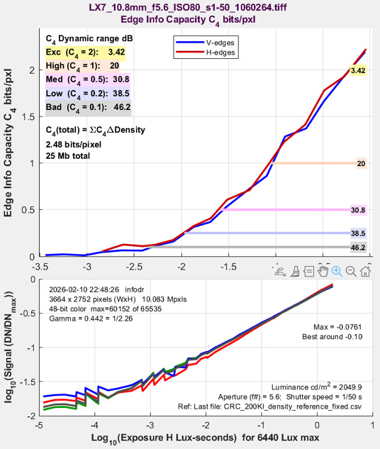
The InfoDR chart is a two-layer transmissive chart, with 3 groups of 7 patches on the top and 3 on the bottom that mirror the top. Adjacent patches in each group are bounded by near-vertical or near-horizontal edges with 4:1 contrast (Density step = ΔD = 0.6). Each group is offset by ΔD =0.2 from its neighbors. The bottom half of the chart is covered with a sheet with D = 2.4. The final chart has 42 patches with 27 distinct density levels and 48 slanted edges (8 in each section; 24 near-horizontal and 24 near-vertical total). The total patch density range is 5.2 (104 dB). The range of mean edge densities is lower by D = 0.6 (12 dB): it is 4.6 (92 dB), which is sufficient for the great majority of cameras
The InfoDR chart is designed to be photographed under the same conditions as the other Dynamic Range charts (darkened room, center of the image, raw capture recommended, etc.).
If the lightbox luminance (candelas/meter2) has been entered, the x-axis of the plot will be in absolute light levels. The value of H = log10(Exposure H Lux-seconds) is identical to the units used in classic film characteristic (Hurter & Driffield) curves.
The upper plot shows C4 (the information capacity for 4:1 contrast objects as a function) of illumination.
Information based dynamic range (based on quality levels Excellent through Bad for C4 = {2, 1, 0.5, 0.25, and 0.1} are shown numerically in the upper-left and as horizontal bars on the right of the upper plot.
C4Δ = ∑C4 ΔDensity is preliminary metric for the overall goodness of the camera. It is close to the maximum information capacity, Cmax, which can be difficult to measure for HDR cameras.
The lower plot shows log(normalized pixel level) as a function of exposure, i.e., the tonal response or OECF (Opto Electronic Conversion Function).
Tips and measurement recommendations
There are a number of things to consider when measuring dynamic range. Most importantly, dynamic range measurements are strongly affected by flare light from the scene (i.e., the chart), image processing (especially bit depth, black level offset, noise reduction, and tone mapping). The experimental setup is critical.
| Light from the environment reflecting back to the front of the test chart should be minimized. It can seriously degrade DR measurements, especially for HDR (DR > 100dB) systems. Be especially careful to avoid reflections from the lens (which should be in the middle of the chart, outside the measurement area). The test environment should be totally darkened. Where possible, walls should be dark. Black cloth should be used to cover lights and light surfaces might reflect light back to the chart. Stray light is the major cause of DR measurement error. |
For 36-patch Dynamic Range or Contrast Resolution charts (shown above) the chart size in the image should be at least 600×600 pixels if possible. For high resolution cameras it doesn’t need to fill the image. A 2000×2000 chart image is more than sufficient for high resolution cameras.
We strongly discourage the use of 20-patch OECF charts, which can have extremely large density steps between the darkest patches, severely compromising measurement accuracy.
Flare light (stray light that reaches the image sensor after bouncing between lens elements and the lens barrel) is the most significant practical limiting factor for DR. It can take the form of fog in shadows (veiling glare) or ghost images (challenging to measure). Flare light can arise from light areas or light sources inside the chart or (in real-world situations) outside the chart. Because of this, the choice of test chart can have a significant effect on DR measurements. Measurement errors caused by flare light are described below.
When possible, DR should be measured in images converted from raw format (the sensor output) with minimal processing and if possible with bit depth of at least 16. This can be done in Imatest using dcraw or Readraw, which do not apply a tonal response curve, sharpening, or noise reduction, hence have relatively little effect on DR.
Dynamic Range can be measured by Color/Tone Interactive, Color/Tone Auto, and Stepchart (legacy module with limited capabilities). Color/Tone Interactive and Auto are recommended because they are newer and have more noise analysis detail than Stepchart.
Image processing can be divided into two categories: processing routinely done during raw conversion and post-processing that is applied afterwards. Both can affect DR measurements.
Raw conversion converts the output of the sensor to a standard image format. It includes several functions (some optional). All the functions listed below are typically applied during in-camera raw conversion (typically with JPEG output). RAW conversion performed in Imatest (using dcraw or Readraw) do not apply a tonal response curve, sharpening, or noise reduction, hence have relatively little effect on DR.
- Demosaicing (converting Bayer RGRG/GBGB format to full color with RGB in each pixel) has relatively little effect on dynamic range.
- Gamma curve Most interchangeable files are gamma-encoded, i.e., they are intended to be displayed with brightness proportional to pixel levelgamma (with gamma typically = 2.2). The simplest gamma encoding is pixel level = scene brightness(1/2.2). When the converted image has a bit depth of 8 (commonplace for non-HDR images), gamma encoding significantly improves dynamic range. 8-bit linear images have limited dynamic range because they have very few levels in dark areas.
- Tonal response curve (TRC). Frequently applied in addition to gamma. A “shoulder” (contrast reduction) applied to the highlights is the most frequent feature of tonal response curves, but dark areas may also be affected. TRCs definitely affect DR measurements (especially slope-based DR), and can do so in complex ways.
- Sharpening is often performed near edges, but may not be applied to flat areas where DR is measured.
- Noise reduction (lowpass filtering) is often performed in flat areas where DR is measured. Noise reduction can have a profound effect on DR measurements— often making them better than reality. SNR = 1, which is a criterion for the DR limit in some standards, may never be reached.
- Color correction matrix (CCM) and white balance (WB). A CCM can increase noise, especially when colors are intensified. But most of the time CCMs have a minor effect on DR measurements.
Additional image processing may be applied following raw conversion.
- Bit depth Most interchangeable images have a bit depth of 8, which can limit DR, especially with linear images. Bit depth = 8 does less harm to gamma-encoded images. Bit depths = 16 or greater has much less effect.
- JPEG High quality JPEG compression has little effect on DR. Low quality JPEG compression messes up DR (and all other image quality measurements), and should never be used for DR measurements. The real issue with JPEGs is that in-camera processing (especially noise reduction, described above) can seriously affect DR and the bit depth of 8 limits DR. The most reliable results are obtained with raw images are converted with minimal image processing to images with a bit depth of 16 or more (48-bit color).
- Tone mapping is performed when HDR images need to be viewed on devices with limited dynamic range (which means pretty much all of them in practice). Tone mapping compresses tones in relatively large areas (such as grayscale test chart patches) while maintaining tonal contrast in small areas (local contrast). It can often be recognized by very low values of gamma (<0.25; well below the value of 0.45 used for most color spaces). It is discussed in the page on the Contrast Resolution chart.
|
Tone mapping makes objects— especially in dark regions— more visible by increasing local contrast (over small areas) while decreasing global contrast (which correlates with measured gamma). It can cause uneven response in grayscale patches, and it can also cause irregularities in the tonal response by breaking the monotonic relationship between pixel level and chart density. This can lead to unexpected results and generally makes a mess of Dynamic Range measurements. We recommend the Contrast Resolution chart for tone-mapped images— or better— completely avoiding tone-mapped images when measuring Dynamic Range. |
Tone mapping reduces contrast measured on standard grayscale charts, which give no indication of how well local contrast is preserved. (The Contrast Resolution chart and analysis were designed to measure local contrast.) Tone mapping can be studied with the Image Processing module, which lets you open any image, add noise noise and other degradations, then apply image enhancements, including three types of tone mapping supported by Matlab (tone mapping, local tone mapping, and Contrast-Limited Adaptive Histogram Equalization). We have found that tone mapping tends to be sensitive to small changes in the noise level. (Of course cameras may use completely different algorithms.)
Tone mapping is fairly easy to identify. Measured gamma is much lower than values typical for standard color space images (around 0.5), and patch levels may not decrease monotonically. The Image Statistics example below shows evidence of tone mapping. The effects of tone mapping on DR measurements are not easy to predict: it should be regarded as a complete wildcard. Dynamic Range measurements of tone-mapped images are not reliable.
The slope-based Dynamic Range (which is sometimes considered total DR because it tends to be larger than SNR-based DR measurements) is defined as the range of exposure where slope of the density curve is greater than 7.5% of the maximum slope (on the dark side) and less than 98% of the saturation level (on the light side). Since tone mapping reduces the maximum slope, it increases the slope-based DR. The slope-based DR often has an extremely low SNR in the dark part of its range, −10 dB or worse, which makes it quite inconsistent, even without tone mapping.
 Pixel level (black level) offsets (pedestals), which are often applied to images, have a significant effect on DR measurements. They can be identified by a flattening of the response curve (log pixel level) in darker patches (though they can be confused with flare light).
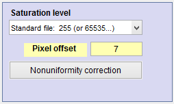
Offsets should be removed if they are present. The default Offset setting is 0. To subtract the offset in Color/Tone Interactive, click the Settings button (if it’s visible) or the Settings dropdown menu, then Color matrix and other settings… The Offset setting is in the lower left of the Settings window. The setting appears in yellow if it’s different from the default value of 0. Offsets can also be corrected during raw conversion with Generalized Read Raw.
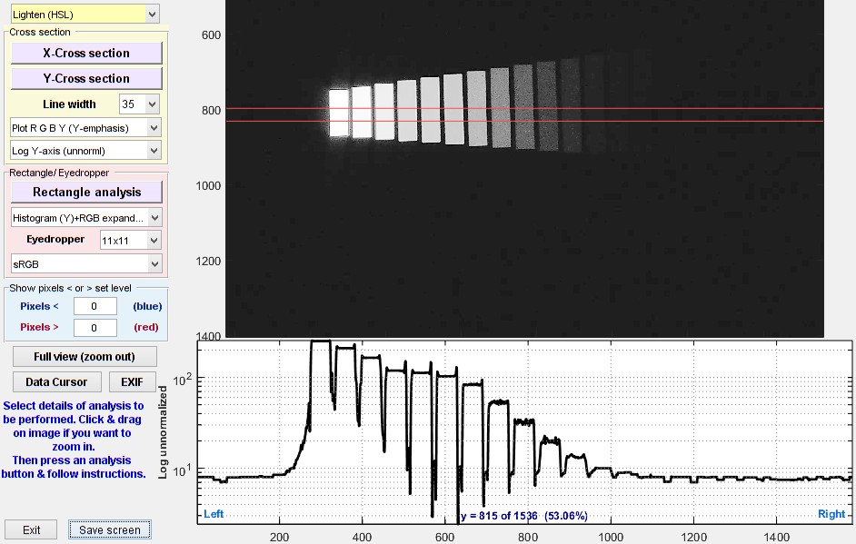
Image Statistics cross-section display showing lightened XYLA chart. A black level offset of 8 bits is likely.
The Image Statistics module can be used to examine the image for tone mapping, flare light, pixel level offsets, and other surprises. It provides information that can be useful when testing DR. The example shows a XYLA chart (a linear chart with density steps = 0.3), which is designed to minimize flare light (the lighter patches are relatively small). The image below is displayed lightened (this does not affect the numeric results below the image). The lower plot is a 35 pixel-wide cross-section of from the chart (averaged to reduce noise). There appears to be a pixel offset of 8 in the black areas outside the chart patches, though it could be long-range flare light (that affects the image uniformly). Some short-range flare light is visible in about 60 pixels to the left of the brightest patch. It’s actually quite well controlled; we’ve seen worse.
The flattening of the response in patches 4-6 indicates that tone mapping has been applied. If it were not caused by tone mapping, this would mean that there would be no image contrast at these densities— an unacceptable result. This is a case where the Contrast Resolution chart provides information that is simply not available from a straight grayscale chart.
More on flare lightFlare light can be extremely complex. It can add a uniform offset to the image (often called “veiling glare”), which is difficult to distinguish from a black level offset. It is often largest near bright patches, then decreases with distance from these patches. The rate of decrease is rarely a well-behaved exponential. This decrease can cause measurement errors because it can falsely resemble changes in chart density. The Image Statistics horizontal cross-section on the right shows the effects of significant flare light on an image of the XYLA chart. Very strong flare light is visible to the left of the chart, and the pixel level continues to drop in areas on the right where chart patches are no longer visible (even when the image is extremely lightened). The lower image— a horizontal cross section of the same image taken below the the chart (displayed with extreme HSL lightening)— shows that this decrease is caused by flare light— not from the camera’s response to the chart. |
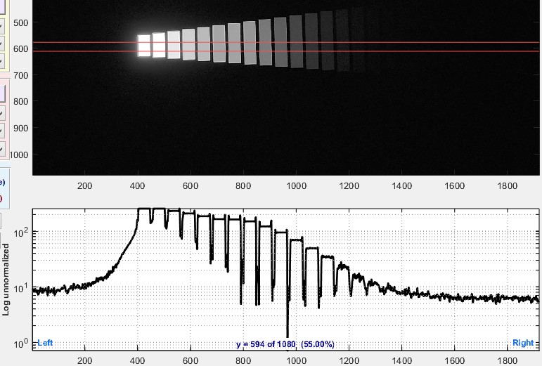 X-cross-section taken at the center of the XYLA chart 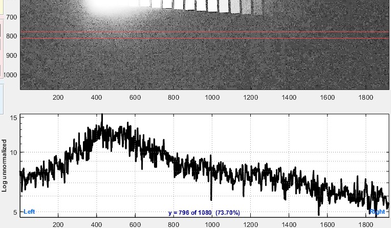 X-cross section taken below the XYLA chart, X-cross section taken below the XYLA chart,showing significant effects of flare light. |
Note that the decrease in pixel level on the right of the chart (around x ≥ 1500) erroneously increases the measured Dynamic Range from slope. The best way to distinguish a pixel level decrease due to flare light from a decrease due to patch densities is with a different chart design, such as the Contrast Resolution chart.
|
Lens reflections are a major cause of medium-range flare light. An uncoated glass surface (index of refraction ≅ 1.5) reflects R = 4% = 0.04 of the light incident on it. (Remember, a sheet of glass or a lens component has two surfaces.)
According to Edmund Optics, the best anti-reflective coatings have R ≅ 0.4% = 0.004 over the visible spectrum (~400-700nm). R = 0.005 may be more realistic for a reasonable range of incident angles. The light reflected back to the sensor from each secondary reflection would be R2 = 0.000025 = 2.5*10-5 = -92 dB (20*log10(R2)). The number of secondary reflections Nsec increases rapidly with the number of components M (groups of elements cemented together, each of which has two air-to-glass surfaces) in a lens: 1 for 1 component; 6 for 2 components; 15 for 3 components; 28 for 4 components; 45 for 5 components, etc. For M components, \(\displaystyle \text{Number of secondary reflections} = N_{sec} = \sum_{i=1}^{2M-1}i = 2M(2M-1)/2 = M(2M-1))\) M = 5 components are typical for high quality camera phones; M ≥12 components is commonplace for DSLR zoom lenses. Overall lens flare is less severe than the number of secondary reflections suggests because the stray light don’t cover the whole image. It decreases with distance from bright regions. It’s easy to see why practical camera Dynamic Range measurements are limited to around 70-90dB, even when sensor Dynamic Range is much higher. 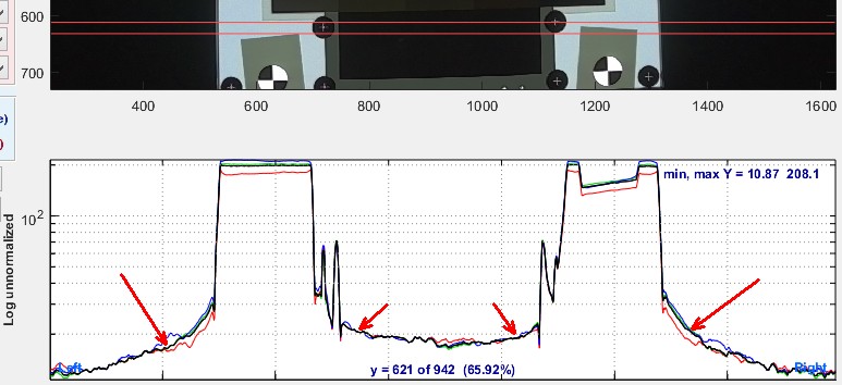 Image Statistics cross-section of a Contrast Resolution image for an automotive camera, showing spatially-varying flare Because the ISO 18844 flare model does not measure the spatially-dependent flare caused by lens reflections, it’s value in characterizing practical system performance is limited. |
Effects of noise
Noise is a random stochastic process. When noise is high in relation to signal level (low SNR), is can have a strong effect on measurement consistency. In particular, the slope-based dynamic range has been discussed in several places above. A key problem with this measurement is that SNR is frequently very low (−10 dB or worse) at its darker limit. (It can also be affected by tone mapping and flare light.) For this reason we don’t recommend its use.
Region selection in linear charts such as the XYLA charts (which have 21 or more f-stops of dynamic range) can be extremely difficult because (a) It is difficult to see dark patches in the denser parts of the causes, (b) it is affected by optical distortion, which can be corrected with difficulty, and (c) it can be affected by keystone distortion (which can also be corrected, but with considerable difficulty). Unfortunately small errors in region selection can significantly affect measurements. This issue was the primary reason we designed the 36-patch Dynamic Range charts (as well as the Contrast resolution chart), both of which have patches arranged in a circular pattern with registration marks for automatic region selection (or easy manual selection if automatic doesn’t work).
Flare light-limited Dynamic Range
The following is an example of a flare light-limited image run in Imatest 5.2. In circular charts (unlike linear charts) flare light drops off in a direction (top to bottom) perpendicular to the patch sequence (left to right) in darker regions. This makes it relatively easy to recognize when the image is being limited by flare light because the density response curve slope drops to zero. This is evident in the upper (density) plot in the image below, where the slope flattens out between 75-100 dB, 105-140 dB, then beyond 145 dB — corresponding to the 6th through 8th rows of patches at the bottom of the chart.
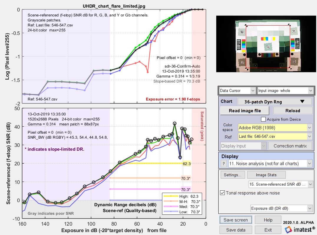 Flare light-limited Dynamic Range result for 36 patch UHDR chart
In this image the scene-reference SNR (dB) stays above 0 to beyond Exposure = -120 dB, but the slope (upper plot) starts to flatten out around -85 dB.Since the pixel level drops to 98% of its maximum level around -15 dB, Dynamic Range is limited to about 70 dB. It would be 120 dB or more without the slope limitation.
Technical details
How is incident light measured?
Incident light has to be measured to obtain the camera’s Exposure Index (ISO Speed).
Reflective charts: Incident light measurement is relatively straightforward. Place an incident illumination meter with a flat diffuser (such as the inexpensive BK615) just in front of the chart, pointed towards the camera, making sure not to block any of the illumination. Use the lux measurement directly.
Transmissive charts: These are not so straightforward: the lux measurement cannot be used directly. You will need to measure a clear (white) area of the chart (not the lightbox itself). For meters like the BK 625, where you can switch the orientation of the sensor, set it to point towards the light source (on the opposite side from the display). Measure the illumination in a white area of the chart. For the 36-patch Dynamic Range chart, use the lightest grayscale patch. You need to make an adjustment because the input to Imatest is designed for reflective charts, where white areas reflect about 90% of the incident light. To compensate for this, use
Lux (input to Imatest) = Lux (measured) * 1.11.
Useful equation: If your meter reads in EV (Exposure Value): Lux = 2.5 * 2EV @ ISO 100
Note: EV @ ISO 100 is also known as Light Value (LV).