Stray light (flare) documentation pages
Introduction: Intro to stray light testing and normalized stray light | Outputs from Imatest stray light analysis | History
Background: Examples of stray light | Root Causes | Test overview | Test factors | Test Considerations | Glossary
Calculations: Metric image | Normalization methods | Light source mask methods | Summary Metrics | Analysis Channels | Saturation
Instructions: High-level Imatest analysis instructions (Master and IT) | Computing normalized stray light with Imatest | Motorized Gimbal instructions
Settings: Settings list and INI keys/values | Standards and Recommendations | Configuration file input
Page Contents
This is the landing page for Imatest’s stray light documentation. This page provides an introduction to stray light and how to test for stray light using the small, bright light source approach. It also introduces the concept of “normalized stray light metric images”. See also the Veiling Glare documentation for information about the chart-based approach to measuring veiling glare; a specific form of stray light.
- Intro to stray light (flare)
- How to test for stray light
- Normalized stray light metric images
- References
Intro to Stray Light (Flare)
What is stray light and how is it measured?
Stray light, also known as flare, is any light that reaches the detector (i.e., the image sensor) other than through the designed optical path (definition from IEEE-P2020 pre-release standard). Stray light can be thought of as systematic, scene-dependent optical noise. Depending on the mechanism causing the stray light, it can produce phantom objects within the scene (i.e., ghosts/ghosting), reduce contrast over portions of the image (e.g., veiling glare), and effectually reduce system dynamic range. These factors can adversely affect the application performance of the camera system in a variety of scenarios. [1]
The stray light of a camera can be measured by capturing images of a bright light source positioned at different angles in (or outside of) the camera’s field of view and then processing those captured images into stray light metric images where each pixel in the image is normalized to represent a stray light metric. The light source object itself is excluded, or masked out in the images, as it is not considered to be stray light. Various information and summary statistics can be derived from the resulting stray light metric images.
Imatest version 22.2 introduced Stray light Source analysis which allows users to generate normalized stray light metric images and other related outputs with high levels of configurability.

A GIF of a series of stray light images captured from a monochrome near-infrared camera paired with a C-mount fisheye lens (FOV >180 degrees). The camera was rotated using the Imatest Motorized Gimbal. These images show a 220-degree horizontal sweep of an infrared collimated light source with about 0.5 degree angular diameter, using field angle increments of 1 degree. Diffraction spikes can be seen immediately surrounding the direct image of the source (these may be categorized as stray light). Some stray light artifacts only appear at specific light source angles, highlighting the importance of test coverage.
How to test for Stray Light
A method to test for stray light involves capturing images of a small, bright light source in a dark room. To build field coverage, the camera can be rotated or the light source can be moved to capture images with at different angles of incident illumination. Using Imatest, the captured images can be processed into “normalized stray light metric images” to objectively measure the magnitude of stray light in the image.
At minimum, to test for stray light, you need:
-
A dark (black) room
-
A small, bright light source (note that the size and focus of the light can impact the form of stray light that it induces in a camera)
-
A way to rotate the camera under test (or a way to move the light source around the camera under test)
Imatest offers several hardware options to help with stray light testing.
Test environment
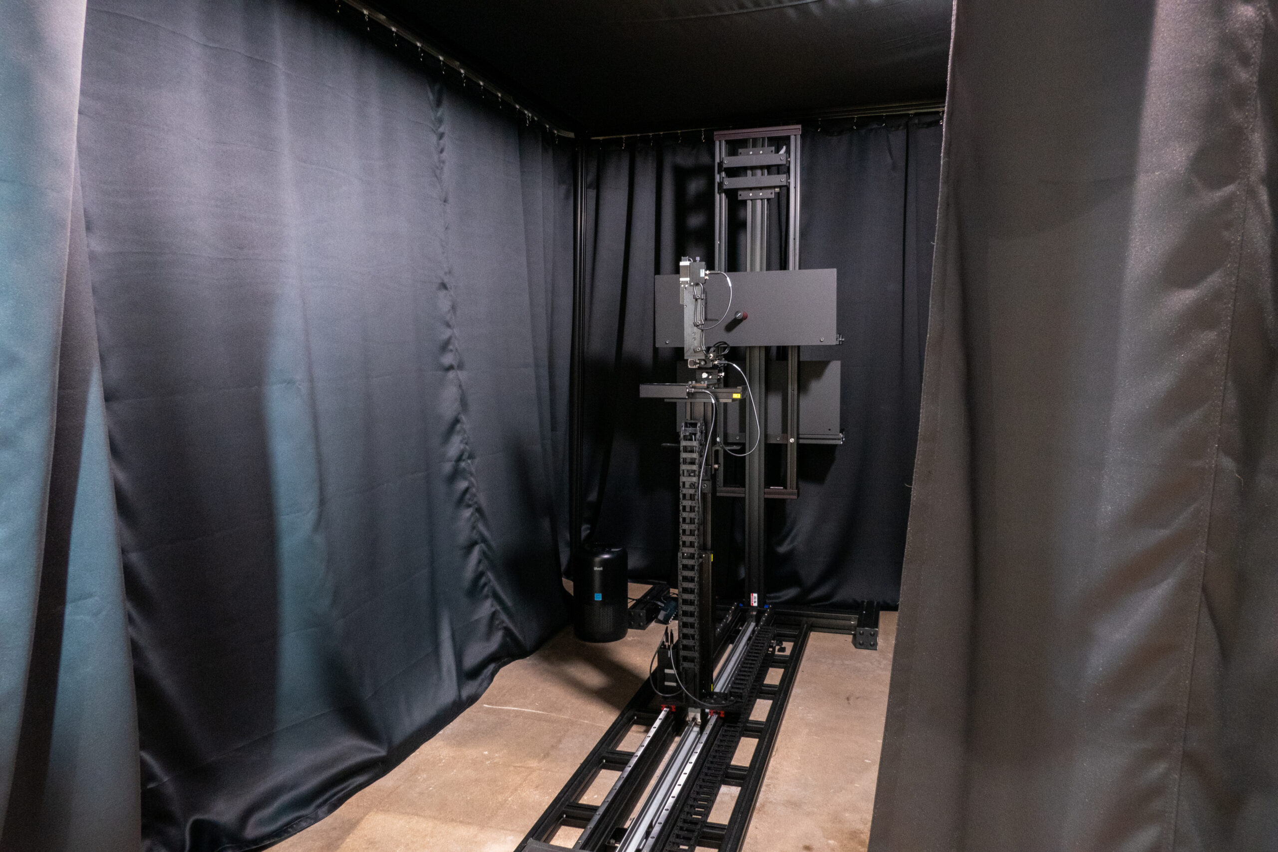
A lab used for stray light testing and development at Imatest’s headquarters. Blackout curtains surround the test fixture to effectively darken the environment.
The ideal environment for a stray light test is an infinitely large and infinitely dark room in a vacuum.
For practical lab testing, it is recommended to use a room with dark/black surfaces. The surfaces of the room may need to be anti-reflective across the full spectrum considered for testing (or the bandpass of the camera). If the room is not dark to begin with, blackout curtains can be used to effectively darken the environment. The blackout curtains should not immediately surround the setup, but rather, there should be some space between the curtains and the setup (camera and light source) to further prevent unwanted reflections. The larger the enclosure, the better. Additional baffles may optionally be used throughout the setup to further reduce extraneous reflections and ambient light.
Ideally, stray light testing should occur in a dustless environment. If there is significant dust on test surfaces (camera or light source) or floating within the beam of light, it may impact the measurement by inducing unwanted reflections and blocking of the light. An air filter can help to achieve a cleaner environment. In addition, a certain level of humidity in the air may help to reduce the amount of floating dust.
Light source, setup, and alignment
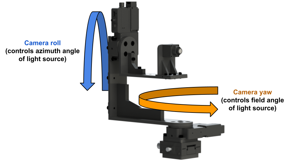
A render of the Imatest Motorized Gimbal with an automotive-grade camera mounted in the stray light test configuration. In this configuration, the gimbal allows for control over the camera roll and yaw, effectively providing control over the field angle and azimuth angle of a light source when properly set up and aligned.
See also the Stray light test overview page for a high-level overview of the test.
For controlled testing, it is generally recommended to use a bright, collimated “point” light source. However, diverging light can be useful if the front of the camera device is significantly large, or if the source of concern for the camera’s application is not at “infinity”.
The light source should be point-like because the angular size of the source can affect the form of stray light in the image. Note that the size of the source in the image is relative to the camera’s instantaneous FOV. Smaller “point sources” produce sharp, high-frequency stray light artifacts, whereas larger “extended sources” produce blurry, low-frequency stray light (akin to veiling glare). This is not to say that point sources cannot cause veiling glare, but rather that extended sources are not likely to cause distinct ghosts. The stray light from an extended source represents a convolution of the stray light from a point source over the area that the extended source subtends. This is a fundamental reason why the chart-based approach to stray light testing is limited to measuring veiling glare [1].
The light emanating from the source should overfill the front of the camera device, including any front surface that could affect the optical path. Using a smaller beam (focused or collimated) that only overfills the front of the camera device helps to reduce the amount of potential extraneous reflections from the setup or test environment. For example, for a phone that has multiple camera modules covered by a protective glass panel, that entire glass panel should be overfilled with light when testing any one of the camera modules, as it’s possible that a stray light path could originate from that surface.
Regarding alignment, the camera should be translationally aligned with the center of the beam of light and the beam should be spatially uniform over the area that illuminates the camera. To find the reference position (often on-axis), corresponding to a field angle of zero, the camera can be rotated to align the direct image of the light source with the “center” of the image (usually the numeric center). See the Normalization compensation section for an example of a reference image.
When rotating a camera or light source, the center of rotation should be the front of the camera or the front-most surface of the device which could affect the optical path. For example, if a camera has a lens hood, the camera should be positioned such that the front end of the lens hood is at the center of rotation. The first reason for doing this is to minimize the necessary area of the projected beam (rotating about a point other than the front could induce a lever arm that would require a larger beam of light to consistently overfill the device at all angles). Another reason for doing this is that the front of the camera device could be the starting point for a stray light path.
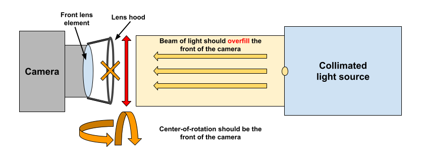
Diagram showing a basic stray light test configuration. The center of rotation should be the front of the camera. The beam of light should overfill the front of the camera.
Test coverage: extent and sampling
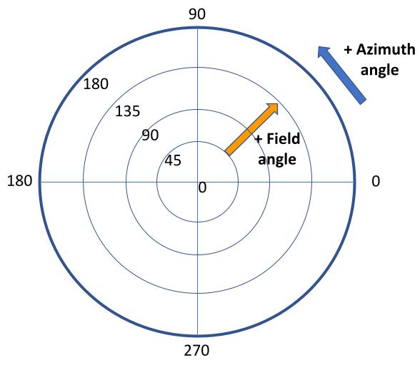
Azimuth angle and field angle represent the position of the light source with respect to the camera. For the purpose of stray light testing, a field angle of zero should coincide with an optical center in image space. For comprehensive testing, it is recommended that the analysis include images where the light source is positioned at field angles beyond the camera’s maximum field of view.
Test coverage is a crucial aspect of stray light testing, encompassing both extent (range) and sampling (delta). Stray light is a high-dimensional problem, in that there are many factors over which it can be measured. Sufficient test coverage is essential for gaining an accurate understanding of the various manifestations of stray light in an image.
The principle of test coverage is somewhat analogous to how sharpness (MTF/SFR) can be measured using only the center of an image, but how this single measurement may not be representative of performance at other locations in the image (e.g., the image corners). Similarly, the most basic form of the stray light test may involve the analysis of a single image of a light source. However, stray light is scene-dependent and therefore, it should be tested with the light source positioned at different angles with respect to the camera. This can include images where the light source is positioned outside the camera’s field of view (FOV).
The position or angle of the light source with respect to the camera can be defined by two attributes: field angle and azimuth angle. A stray light “capture plan” can be defined as a series of positions with these two attributes. For Imatest stray light analysis, the light source azimuth angle and field angle for each input image can be defined and referenced for analysis via a Configuration file.
An example of a simple stray light capture plan is a single-axis sweep of the light source, wherein the camera is rotated (or the light source moved) such that the light source covers an arc across the full FOV of the camera (e.g., a 180-degree arc). Note that for comprehensive testing, field angle increments of 1 degree or less may be necessary to reveal all stray light paths, depending on the FOV of the camera. Also note that certain stray light paths caused by dust, lens surface defects, or other asymmetries in the opto-mechanical design of a camera may lead to asymmetric stray light performance.
Comprehensive testing may involve multi-axis sweeps of the light source, wherein the camera is rotated to perform multiple sweeps at several azimuth angles. For example, a valid capture plan could be to test at field angles ranging from 0 to 90 degrees with 0.1-degree increments, at azimuth angles corresponding to horizontal, vertical, and diagonal, where the diagonal angle intersects with the corners of the image.

A GIF of a multi-axis sweep of a light source with a camera showing significant “petal flare”. The camera was rotated using the Imatest Motorized Gimbal in order to capture a series of images with the light source positioned at multiple azimuth angles and field angles with respect to the camera, including field angles where the light source is outside the camera’s field of view.
A fundamental assumption of normalized stray light is that the input data is linear. Certain image signal processing (ISP), especially those affecting linearity (e.g., gamma correction), can impact the measurement by affecting the relative stray light response in the image. Nevertheless, processed images may be analyzed as well, since it can be valuable to see how a camera’s ISP impacts the perceived stray light.
The Imatest stray light analysis supports input image files containing monochrome or 3-channel (e.g., RGB) image data. Unformatted raw images are also supported with the use of Read Raw settings. Supported files are described in Image file formats and acquisition devices.
Normalized stray light metric images
The primary output from the Imatest stray light analysis are stray light metric images. The stray light metric images can be output as FITS files and as color-mapped plots (saved as image files and/or video files).
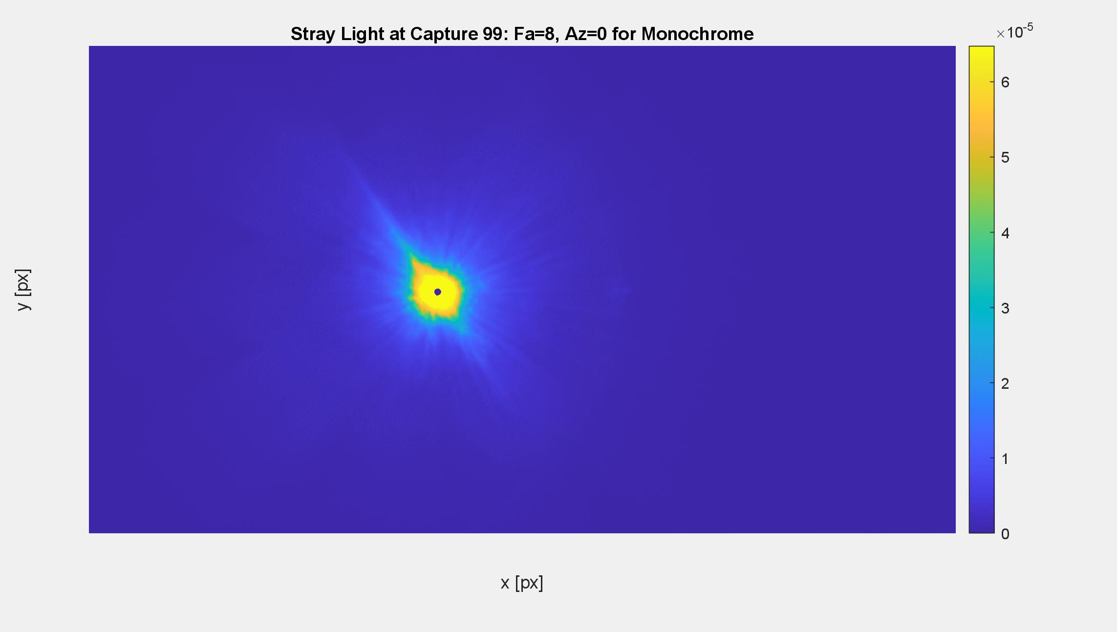
A color-mapped plot of a normalized stray light metric image. The input linear image data has been normalized by the level (digital number/pixel value) of the direct image of the light source from a separate reference image. For the reference image, we used a shorter exposure time and attenuated the light source with a neutral density filter such that the direct image of the source was not saturated. We computed the mean level from within the direct image of the source in the reference image. We then compensated for the difference in light level between the reference image and test image to compute a theoretical level above saturation as the final “compensated” normalization factor. Here, the level of stray light in the metric image is measured to be around 0.0006% or less of the level from the direct image of the source, although the saturated stray light (yellow) is likely greater in magnitude. The light source in use has an angular diameter of about 0.5 degrees (similar to the Sun) and the computed metric is Extended Source Rejection Ratio (ESRR) [2]. The direct image of the source is masked out because it is not stray light.
Normalized stray light background
For analysis in Imatest, the input should be linear images of a small, bright light source (e.g., a point-like source) in a completely dark room. A key assumption of the test is that any response in these images is stray light, other than the response from the direct image of the source. The direct image of the source is the small region in the image that represents the actual size of the light source (i.e., if there were no stray light or blooming in the image) [1]. The direct image of the source is masked out (ignored) during analysis because it is not stray light.
Using Imatest, each pixel in the input images can be normalized to represent a stray light metric, wherein the method of normalization determines the metric. At a high level, the normalized stray light calculation can be written quite simply as:
$$\text{normalized stray light} = \frac{\text{input image data [DN]}|}{\text{normalization factor [DN]}}$$
Note that this form of the equation corresponds with stray light transmission, while the reciprocal would correspond with stray light attenuation.
The primary normalization method supported by Imatest is to normalize by the image level (mean digital number (DN) or pixel value) from within the direct image of the light source. With this method, the values in the metric image are representative of the level/response of stray light in the image relative to the level/response directly from the light source. If testing with a point light source, this normalization method would correspond to the Point Source Rejection Ratio (PSRR) metric [2]. If testing with an extended source, the metric would be the Extended Source Rejection Ratio (ESRR) [2]. The Sun, for example, is an extended source at “infinity” with an angular diameter of about 0.53 degrees, unlike other further away stars which are perceived as point sources. The angular size of the light source can determine the form of stray light manifested in an image, which is one of the fundamental reasons for performing this type of test with a small, bright light source.
Normalization compensation
Another key assumption of the test is that the level used to normalize the test image data (i.e., the normalization factor) is below saturation. Saturation, or the dynamic range of the camera under test, inherently limits the dynamic range of the test itself. Normalizing by saturation level provides relatively meaningless results because the level of saturated data is ambiguous. If normalizing by saturation, the resulting metric image will have values ranging from 0 to 1 where 1 corresponds to the saturation level. For many cameras, the direct image of the source may need to be saturated in order to induce stray light in the image. In this case, we can use the information from separate well-exposed reference images where the light level has been attenuated such that the direct image of the source is not saturated. Depending on the controls available to the camera, there are different techniques that can be used to produce an unsaturated image of the source and then a “test image-equivalent” (compensated) normalization factor, such as [1]:
- Adjust the exposure time \(t\)
- Adjust the system gain \(\rho\)
- Adjust the source light level \(L\), e.g., with ND filters and/or
direct control of light source power
These techniques can be used individually or combined to form a compensation factor \(C\) that would serve as a multiplier for the base normalization factor \(N_{base} \) to compute a compensated normalization factor \(N_{compensated} \) (which is finally used to normalize the test image data). In this case, the base normalization factor \(N_{base} \) is the image level (digital number or pixel value) of the direct image of the source from the reference image [1]. The overall process can be described with a few simple equations:
$$\text{normalized stray light} = \frac{\text{input image data [DN]}}{N_{compensated}\text{[DN]}}$$
where \(N_{compensated} = N_{base}\cdot C\)
and \(C = \frac{t_{test}}{t_{reference}}\cdot\frac{\rho_{test}}{\rho_{reference}}\cdot\frac{L_{test}}{L_{reference}} \)
Note that these techniques assume that the camera data is linear or linearizable and that the reciprocity law holds [1]. The following section provides an example of normalized stray light calculation with use of a compensation factor.
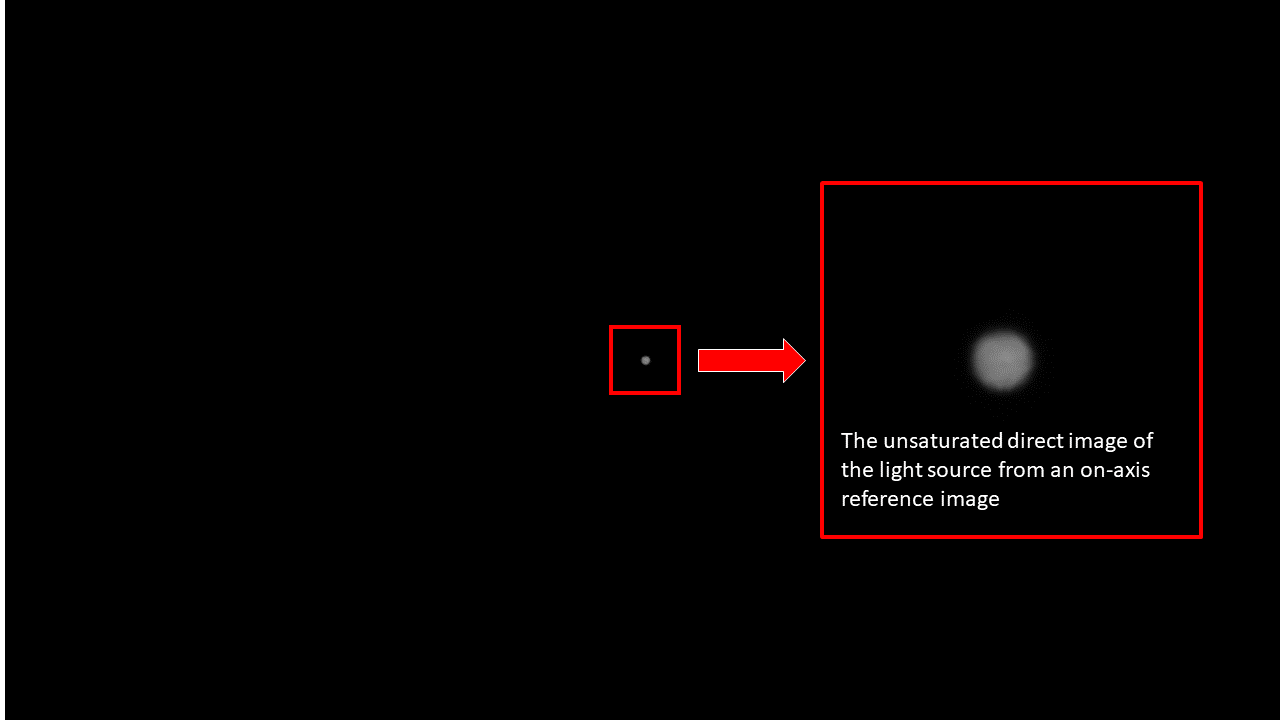
Figure 2: A reference image showing an unsaturated direct image of the light source. The image was captured using a shorter camera exposure time than the test images and with an ND 2.5 filter in front of the light source. In the separate test images (not shown), the direct image of the source is saturated and significantly blooming to reveal stray light.
Interpreting normalized stray light metric image data
Consider the following example test procedure for a camera that outputs linearized 16-bit image data:
- For the test images, we set the level of our light source and the exposure of our camera to 100ms duration such that significant measurable stray light artifacts appear in the image. However, the direct image of the source is saturated in these images.
- For the reference image, we set our camera to its minimum exposure of 1ms and place an ND filter with a density of 2.5 (transmission = 10^(-2.5) = 0.316%) in front of our source to attenuate the light such that the direct image of the source is not saturated in the image.
- We measure the (mean) level within the direct image of the source from the reference image. We measure an average unsaturated level (pixel value) of 31941.617. This is the base normalization factor \(N_{base} \) that we will use to normalize our test image data.
- We compensate the base normalization factor to compute a “test image-equivalent” normalization factor, by taking the ratio of the test image light level and the reference image light level through the use of the known ND filter transmission and exposure difference. The compensation factor is: \(C = \frac{100\%}{0.316\%}\cdot 100ms= 31645.6 \). The compensated normalization factor is: \(N_{compensated} = N_{base}\cdot C = 1010082618.74 \). This normalization factor is in units of DN (digital number or pixel value). Hence, we are essentially normalizing by a theoretical pixel value above the saturation level.
- As a step in the calculation of the metric image, we mask out (ignore, set to NaN) the direct image of the source in the test image(s) because it is not stray light.
- We compute the normalized stray light metric image: \( \text{normalized stray light} = \frac{\text{input image data [DN]}}{N_{compensated}\text{[DN]}} \)
Looking at the result, we see that the values in the stray light metric image range from 0 to 6.476E-5. This tells us that the maximum response of stray light in the image is measured to be about 0.0006476% of the response from the direct image of the source. Here, a value of 6.476E-5 corresponds to image data that is saturated (for this camera’s image data, the saturation level is 65408 and when divided by \(C\) we get 6.476E-5). Stray light at this level has lost meaning, since we do not have the ability to measure data that is saturated. Specifically, the saturated stray light is likely greater in magnitude than what can be measured. However, the data that is not saturated (corresponding to stray light values less than 6.476E-5) are still meaningful to us. Again, these normalized stray light values represent the stray light response relative to the direct light source response. If the data are truly linear and if reciprocity law holds, we can infer that these normalized values will not change significantly if we use a light source of different intensity or different camera exposure time. Though different exposure times or light source intensities can still reveal different magnitudes of stray light for us to measure (e.g., longer camera exposure time will reveal fainter stray light artifacts).
The question of what is an acceptable level of stray light may depend on the application of the camera. This is similar to asking the question “what is an acceptable MTF measurement” which is also relatively ambiguous and depends on the system application. Nevertheless, we can consider the properties of the light sources of concern for the camera to determine an acceptable level. Take for example the Sun, which is a small, bright light source, and consider the following example for a camera with an ADAS/automotive application [1]:
- In application, the camera operates with exposure time T while the Sun is in the field of view with an average irradiance of E on the camera.
- The intent of the test is to simulate the application stray light performance, but the test light source level is measured to be only \(\frac{E}{10} \).
- Assuming linearity and reciprocity, the camera can be tested with exposure time T x 10 to simulate the application’s stray light performance.
In the resulting test images, the level of stray light should correspond with the level of stray light in the application. However, it is still up to the user to decide the acceptable level.
The acceptable level of stray light may also depend on the exposure algorithm of the camera system. For a given camera, different auto-exposure algorithms or metering techniques can be used to expose for a given scene, allowing for different levels of saturation. For example, if the camera’s exposure algorithm prevents the image from ever reaching saturation, the acceptable level of stray light may be more than if the exposure algorithm accepts significant amounts of saturation and blooming (at which point, we may see more stray light). Additionally, a camera that operates in low light may be more concerned with lower levels of stray light. So, keeping with the same example, this means that a normalized stray light value of 6.476E-5 may be problematic for some cameras and scenarios, but not for others.
Overall, the stray light metric images may need to be analyzed both objectively and subjectively. Objective analysis may include looking at the measured level of stray light and deriving statistics based on the stray light metric image data (e.g., various statistics plotted as a function of light source field angle). Subjective analysis may involve visually inspecting the image data to see if the color, shape, and size of the stray light artifacts are negatively affecting image quality and/or checking if those artifacts could impact the application of the camera. For example, are there any sharp ghost artifacts that could resemble real concerning objects (e.g., traffic light signals), or are they simply unappealing/distracting to a viewer? Is there significant veiling glare and how could it affect the contrast resolution or MTF of the system? Could any of the stray light artifacts in the image potentially lead to system failure scenarios?
References
[1] Jackson S. Knappen, “Comprehensive stray light (flare) testing: Lessons learned” in Electronic Imaging, 2023, pp 127-1 – 127-7, https://doi.org/10.2352/EI.2023.35.16.AVM-127