Introduction – Encoding vs. Display gamma – Why logarithms?
How gamma-encoding increases dynamic range – Expected gamma values – Entering gamma into Imatest
Gamma and MTF – The effects of gamma errors on MTF
Which patches are used to calculate gamma? – Why gamma ≅ 2.2? – Why are raw-converted images often dark?
Tone mapping – Contrast definitions: Ratio, Weber, Michelson – Logarithmic color spaces – Monitor gamma
Introduction
In this post we discuss a number of concepts related to tonal response and gamma that are scattered around the Imatest website, making them hard to find. They are assembled here in anticipation of questions about gamma and related concepts, which keep arising.
Gamma (γ) is the average slope of the function that relates the logarithm of pixel levels (in an image file) to the logarithm of exposure (in the scene).
\(\text{log(pixel level)} \approx \gamma \ \text{log(exposure)}\)
This relationship is called the Tonal Response Curve, (It’s also called the OECF = Opto-Electrical Conversion Function). The average is typically taken over a range of pixel levels from light to dark gray.
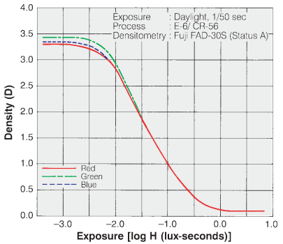
Tonal Response Curve for Fujichrome Provia 100F film. The y-axis is reversed from the digital plots.
Tonal Response Curves (TRCs) have been around since the nineteenth century, when they were developed by Hurter and Driffield— a brilliant accomplishment because they lacked modern equipment. They are widely used for film. The Tonal Response Curve for Fujichrome Provia 100F film is shown on the right. Note that the y-axis is reversed from the digital plot shown below, where log(normalized pixel level) corresponds to \(D_{base} – D\text{, where } D_{base} = \text{base density} \approx 0.1\).
Equivalently, gamma can be thought of as the exponent of the curve that relates pixel level to scene luminance.
\(\text{pixel level = (RAW pixel level)}^ \gamma \approx \text{exposure} ^ \gamma\)
There are actually two gammas:
-
encoding gamma, which relates scene luminance to image file pixel levels, and
-
display gamma, which relates image file pixel levels to display luminance. It is typically found in equations of the form,
The equation, (above and in most references to gamma on this page), refers to encoding gamma. Exceptions are for characterizing color spaces (such as sRGB, where display gamma is approximately 2.2) and when display gamma is explicitly referenced, as in the Appendix on Monitor gamma.
The overall system contrast is the product of the encoding and decoding gammas. More generally, we think of gamma as contrast.
Encoding gamma is applied in the image processing pipeline because the output of image sensors, which is linear for most standard (non-HDR) image sensors, is never gamma-encoded. Encoding gamma is typically measured from the tonal response curve, which can be obtained photographing a grayscale test chart and running Imatest’s Color/Tone module (or the legacy Stepchart and Colorcheck modules).
Display gamma is typically specified by the color space of the file. For the most common color space in Windows and the internet, sRGB, display gamma is approximately 2.2. (It actually consists of a linear segment followed by a gamma = 2.4 segment, which together approximate gamma = 2.2.) For virtually all computer systems, display gamma is set to correctly display images encoded in standard (gamma = 2.2) color spaces.
Here is an example of a tonal response curve for an in-camera JPEG for a high quality consumer camera, measured with Imatest Color/Tone.
 Tonal response curve measured by the Imatest Color/Tone module
from the bottom row of the 24-patch Colorchecker,
Note that this curve is not a straight line. It’s slope is reduced on the right, for the brightest scene luminance. This area of reduced slope is called the “shoulder”. It improves the perceived quality of pictorial images (family snapshots, etc.) by reducing saturation or clipping (“burnout”) of highlights, thus making the response more “film-like”. A shoulder is plainly visible in the lower-right of the Fujichorme Provia 100F curve, above. Shoulders are almost universally applied in consumer cameras; they’re less common in medical or machine vision cameras. [A region of reduced slope in dark regions is called a “toe”. It is common in film, but relatively rare in digital images.]
Because the tonal response is not a straight line, gamma has to be derived from the average (mean) value of a portion of the tonal response curve.
Why use logarithms?
Logarithmic curves have been used to express the relationship between illumination and response since the nineteenth century because the eye’s response to light is logarithmic. This is a result of the Weber-Fechner law, which states that the perceived change dp to a change dS in an initial stimulus S is
\(dp = dS/S\)
Applying a little math to this curve, we arrive at where ln is the natural logarithm (loge).
From G. Wyszecki & W. S. Stiles, “Color Science,” Wiley, 1982, pp. 567-570, the minimum light difference ΔL that can be perceived by the human eye is approximately
\(\Delta L / L = 0.01 = 1\% \). This number may be too stringent for real scenes, where ΔL/L may be closer to 2%.
The brighter areas take up far too much space in linearly-displayed tonal response curves, making it difficult to see the response in darker areas.
How gamma encoding increases Dynamic Range
In photography, we often talk about zones (derived from Ansel Adams’ zone system). A zone is a range of illumination L that varies by a factor of two, i.e., if the lower and upper boundaries of a zone are L1 and L2, then L2 /L1 = 2 or log2(L2) – log2(L1) = 1.
| 1 | 2 | 3 | 4 | 5 | 6 | 7 | 8 | 9 |
|
|
The steps between each zone has equal visual weight, except for very dark zones where the differences are hard to see.
For a set of zones z = {1, 2, 3, ..} the relative illumination of zone n is 2-(z-1) = {1, 0.5, 0.25, 0.125, …}. The illumination difference between zones is {0.5, 0.25, 0.125, …}. The scene illumination ratio is always 2:1.
|
Geek alert: a lot of numbers follow— all of which are intended to show how gamma encoding increases the effective dynamic range. The total number of available pixel levels B is a function of the bit depth, B = 2(bit depth). For bit depth = 8, B = 256; for bit depth = 16, B = 65536. The relative pixel level of zone n for encoding gamma γe is bn = B × 2-(n-1)γe.For linear gamma (γe = 1), bn= {1.0, 0.5, 0.25, 0.125, …} (the same as L). For γe= 1/2.2 = 0.4545, bn = {1.0000, 0.7297, 0.5325, 0.3886, 0.2836, 0.2069, 0.1510 ,0.1102, …}. The relative pixel levels bn decrease much more slowly than for γe = 1. The relative number of pixel levels in each zone is npγ(i) = bn(i) – bn(i+1), which brings us to the heart of the issue. For a maximum pixel level of 2(bit depth)-1 = 255 for widely-used files with bit depth = 8 (24-bit color), the total number of pixels in each zone is Npγ(i) = 2(bit depth)npγ(i).  When gamma = 2.2, the darker zones in the file contain more pixel levels. For linear images (γe = 1), npγ(i) = {0.5, 0.25, 0.125, 0.0625, …}, i.e., half the pixel levels would be in the first zone, a quarter would be in the second zone, etc. For files with bit depth = 8, the zones starting from the brightest would have Npγ(i) = {128, 64, 32, 16, 8, 4, 2, 1 …} pixel levels of 256 (0-255). By the time you reached the 5th or 6th zone, the spacing between pixel levels would be small enough to cause significant “banding”, limiting the dynamic range. For images encoded with γe = 1/2.2 = 0.4545, the relative number of pixels in each zone would be bn(i) = {0.2703, 0.1972, 0.1439, 0.1050, 0.0766, 0.0559, 0.0408, 0.0298, 0.0217, 0.0159…}, and the total number Npγ(i) would be {69.2, 50.5, 36.8, 26.9, 19.6, 14.3, 10.4, 7.63, 5.56, 4.06, …} of 256. The sixth zone, which has only 4 levels for γe = 1, has 14.3 levels. The 10th gamma-encoded zone has the same number of levels (4) as the 6th linear zone, i.e., an effective dynamic range increase of up to four zones (f-stops; factors of 2). To summarize: Of course, the improvement will be less if flare light in dark regions is the limiting factor. |
What gamma (and Tonal Response Curve) should I expect?
And what is good?
JPEG images from consumer cameras typically have complex tonal response curves (with shoulders), with gamma (average slope) in the range of 0.45 to 0.6. This varies considerably for different manufacturers and models. The shoulder on the tonal response curve allows the the slope in the middle tones to be increased without worsening highlight saturation. This increases the apparent visual contrast, resulting in “snappier” more pleasing images.
RAW images from consumer cameras have to be decoded using LibRaw/dcraw. Their gamma depends on the Output gamma and Output color space settings (display gamma is shown in the settings window). Typical results are
-
Encoding gamma ≅ 0.4545 with a straight line TRC (no shoulder) if conversion to a color space (usually sRGB or Adobe RGB) is selected;
-
Encoding gamma ≅ 1.0 if a minimally processed image is selected.
RAW images from binary files (usually from development systems) have straight line gamma of 1.0, unless the Read Raw Gamma setting (which defaults to 1) is set to a different value.
Flare light can reduce measured gamma by fogging shadows, flattening the Tonal Response Curve for dark regions. Care should be taken to minimize flare light when measuring gamma.
That said, we often see values of gamma that differ significantly from the expected values of ≅0.45-0.6 (for color space images) or 1.0 (for raw images without gamma-encoding). It’s difficult to know why without a hands-on examination of the system. Perhaps the images are intended for special proprietary purposes (for example, for making low contrast documents more legible by increasing gamma); perhaps there is a software bug.
What effect does entering gamma have on Imatest measurements?
Gamma can be entered into imatest in several places. Here is what it does, and equally important, what it does not do.
Gamma can be measured from grayscale test charts. Entered values of gamma do not affect grayscale measurements.
- Gamma is used to linearize images for MTF calculations. The entered value of gamma can be overridden for slanted-edge patterns if the pattern contrast ratio (often 4) has been entered and Use for MTF has been checked.
- In Flatfield, gamma is used to linearize ISO 18844 flare light measurements and also to calculate F-stop contour plots (not one of Imatest’s major displays; luminance (pixel) contour plots are usually preferred.)
- In Color/Tone, gamma is used to linearize the image for calculating the Color Correction Matrix (important) and for correcting illumination nonuniformity (an infrequently-used feature that requires a second flat image).
Gamma and MTF measurement
MTF (Modulation Transfer Function, which is equivalent to Spatial Frequency Response), which is used to quantify image sharpness, is calculated assuming that the signal is linear. For this reason, gamma-encoded files must be linearized, i.e., the gamma encoding must be removed. The linearization doesn’t have to be perfect, i.e., it doesn’t have be the exact inverse of the tonal response curve. For most images (especially where the chart contrast is not too high), a reasonable estimate of gamma is sufficient for stable, reliable MTF measurements. The settings window for most MTF calculation has a box for entering gamma (or setting gamma to be calculated from the chart contrast).
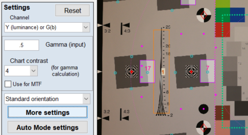
Gamma is entered in the Setup or More settings window for each MTF module. They are described in the documentation for individual Rescharts modules. For Slanted-edge modules, they appear in the Setup window (crop shown on the right) and in the More settings window (crop shown below).
![]()
Gamma (input) defaults to 0.5, which is a reasonable approximation for color space files (sRGB, etc.), but is incorrect for raw files, where gamma ≅ 1. Where possible we recommend entering a measurement-based estimate of gamma.
Determine gamma from a grayscale pattern
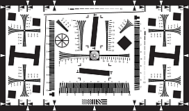
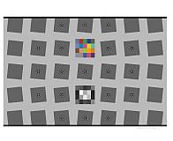
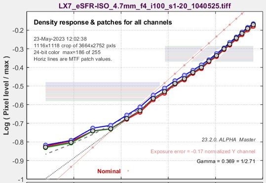
Gamma is often measured from grayscale (OECF) patterns, which can be in separate charts or included in any of several sharpness charts— SFRplus, eSFR ISO, Star, Log F-Contrast, and Random (but not Checkerboard). The grayscale pattern from the eSFR ISO and SFRplus chart is particularly interesting because it shows the levels of the light and dark portions of the slanted-edge patters used to measure MTF.
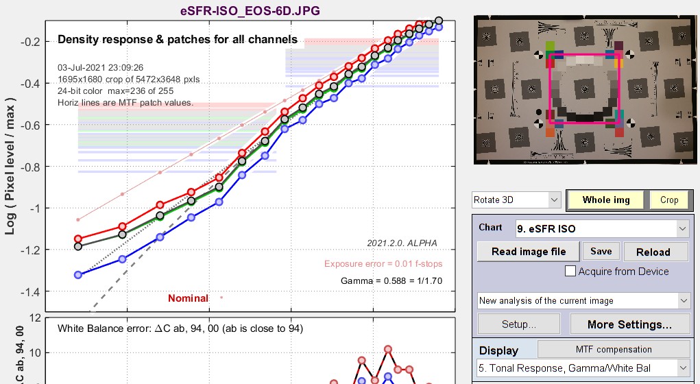 Tonal response plot from eSFR ISO chart
Gamma = 0.588 here: close to the value (shown above) measured from the X-Rite Colorchecker for the same camera. The interesting thing about this plot is the pale horizontal bars, which represent the pixel levels of the light and dark portions of the selected slanted-edge ROIs (Regions of Interest). This lines let you see if the slanted-edge regions are saturating or clipping. This image shows that there will be no issue.
Determine gamma from each individual slanted-edge
Enter chart contrast and check Use for MTF. Only available for slanted-edge MTF modules.
Enter chart contrast and check Use for MTF. Only available for slanted-edge MTF modules. When Use for MTF is checked, the gamma (input) box is disabled.
This setting uses the measured of contrast of flat areas P1 and P2 (light and dark portions of each individual slanted-edge Region of Interest (ROI), away from the edge itself) to calculate the gamma for each edge. It is easy to use and quite robust. The printed chart contrast ratio (<=10) must be entered and the OECF curve should be close to \(\text{log(P)} \approx \gamma_{encoding} \ \text{log(exposure)}\).
\(\displaystyle gamma\_encoding = \frac{\log(P_1/P_2)}{\log(\text{chart contrast ratio)}}\)
|
A brief history of chart contrast
This issue was finally corrected with ISO 12233:2014 (later revisions are relatively minor), which specifies a 4:1 edge contrast, which not only reduces the likelihood of clipping, but also makes the MTF calculation less sensitive to the value of gamma used for linearization. The old ISO 12233:2000 chart is still widely used: we don’t recommend it.
Imatest chrome-on-glass (CoG) charts have a 10:1 contrast ratio: the lowest that can be manufactured with CoG technology. Most other CoG charts have very high contrast (1000:1, and not well-controlled). We don’t recommend them. We can produce custom CoG charts quickly if needed. |
How strongly does gamma affect MTF? i.e., if the estimate of gamma is incorrect, how far off is the MTF?
We ran an image from a compact digital camera, converted from raw with dcraw, with a number of different gamma settings to see how the settings affected MTF rsults.
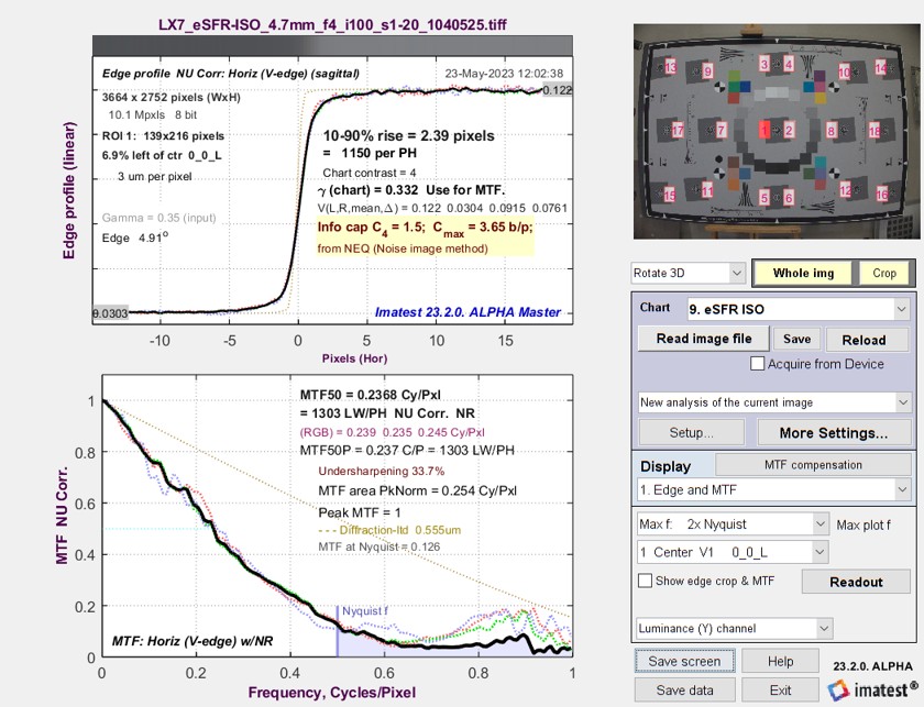 Edge response and MTF. Gamma from chart = 0.332 Edge response and MTF. Gamma from chart = 0.332 |
The chart and images are several years old. The chart may have been printed with lower contrast than intended, resulting in a lower gamma measurement. This has no effect on the relative measurements below. |
| Gamma | MTF50 (C/P) | MTF Area PkNorm (C/P) |
| 0.20 | 0.2415 | 0.261 |
| 0.30 | 0.2408 | 0.258 |
| 0.322 | 0.2368 | 0.254 |
| 0.40 | 0.2387 | 0.254 |
| 0.50 | 0.2344 | 0.247 |
| 0.60 | 0.2332 | 0.247 |
Note that errors in estimating gamma (differences from 0.322) have very little effect on MTF measurements. MTF50 and MTF Area change very slightly, even with relatively large gamma errors. This is a good place discuss Imatest’s ISO 12233 compliance. Imatest uses a simple first-order inverse of the OECF curve (tonal response) measurement to linearize the image. It does not use a higher-order inverse. But because MTF is relatively insensitive to gamma (the slope of the tonal response curve), the simple fit results in nearly identical MTF measurements (except the the exposure is close to saturation, which where it’s hard to avoid dodgy results).
Which patches are used to calculate gamma?
This is an important question because gamma is not a “hard” measurement. Unless the Tonal Response Curve says pretty close to a straight line log pixel level vs. log exposure curve, its measured value depends on which measurement patches are chosen. Also, there have been infrequent minor adjustments to the patches used for Imatest gamma calculations— enough so customers occasionally ask about tiny discrepancies they find.
Light and dark patches where the tonal response curve flattens out are generally omitted from gamma calculations.
For the 24-patch Colorchecker, patches 2-5 in the bottom row are used (patches 20-23 in the chart as a whole).
For all other charts analyzed by Color/Tone or Stepchart, the luminance Yi for each patch i (typically 0.2125×R + 0.7154×G + 0.0721×B) is found, and the minimum value Ymin, maximum value Ymax, and range Yrange = Ymax – Ymin is calculated.
Gamma is calculated from patches where Ymin + 0.2×Yrange < Yi < Ymax – 0.1×Yrange . This ensures that light through dark gray patches are included and that saturated patches are excluded.
History: where did gamma ≅ 2.2 come from?
It came from the Cathode Ray Tubes (CRTs) that were universally used for television and video display before modern flat screens became universal. In CRTs, screen brightness was proportional to the control grid voltage raised to the 2 to 2.5 power. For this reason, signals had to be encoded with the approximate inverse of this value, and this encoding stuck. As we describe above, in “What is gained by applying a gamma curve?”, there is a real advantage to gamma encoding in image files with a limited bit depth, especially 8-bit files, which only have 256 possible pixel levels (0-255).
Why are images converted from raw files often darker
then JPEGs from the same capture?
Many cameras have the option of producing both interchangeable image files (usually JPEG) and raw files from the same image capture. The raw-converted files are frequently darker— sometimes much darker— than the corresponding JPEGs. This is not an accident.
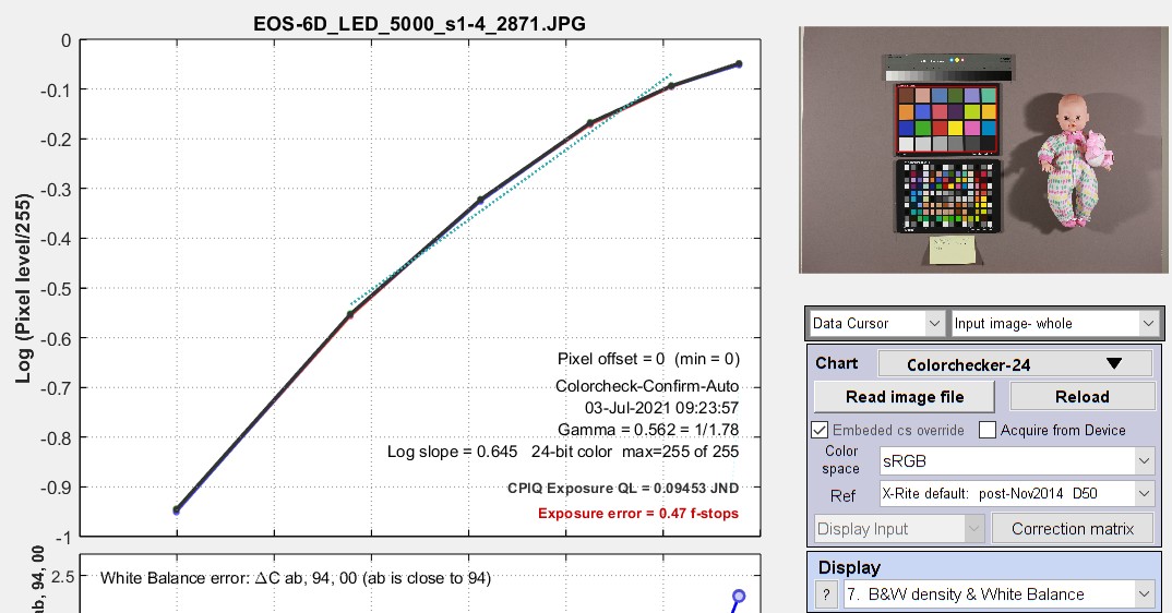
In Imatest, raw files are typically converted to interchangeable files (usually TIFF) using LibRaw, which has several presets and additional options. The most commonly-used presets are Color 24-bit sRGB (gamma ≅ 2.2) and Color 48-bit Adobe RGB (gamma = 2.2). These settings use EXIF metadata in the raw file to perform white balance and color correction (for the selected color space) and apply an appropriate straight-line gamma curve, . The tonal response curve, displayed logarithmically, is a straight line with no “shoulder” or other curvature.
JPEGs, on the other hand, frequently have a “shoulder”— a region where gamma (contrast) is gradually reduced— in the highlights. The shoulder improves the perceived pictorial quality of the image by reducing saturation (or “burnout”) of the highlights. It was a part of film response curves, long taken for granted. In order to achieve this shoulder, the exposure has to be reduced below the optimum level for a straight gamma curve to allow some “headroom” for the shoulder (before highlights are saturated). Here is an example: in-camera JPEG and LibRaw-converted raw images of the Colorchecker charts and doll, whose tonal response curve are shown above or the in-camera JPEG and below for the LibRaw-converted TIFF.
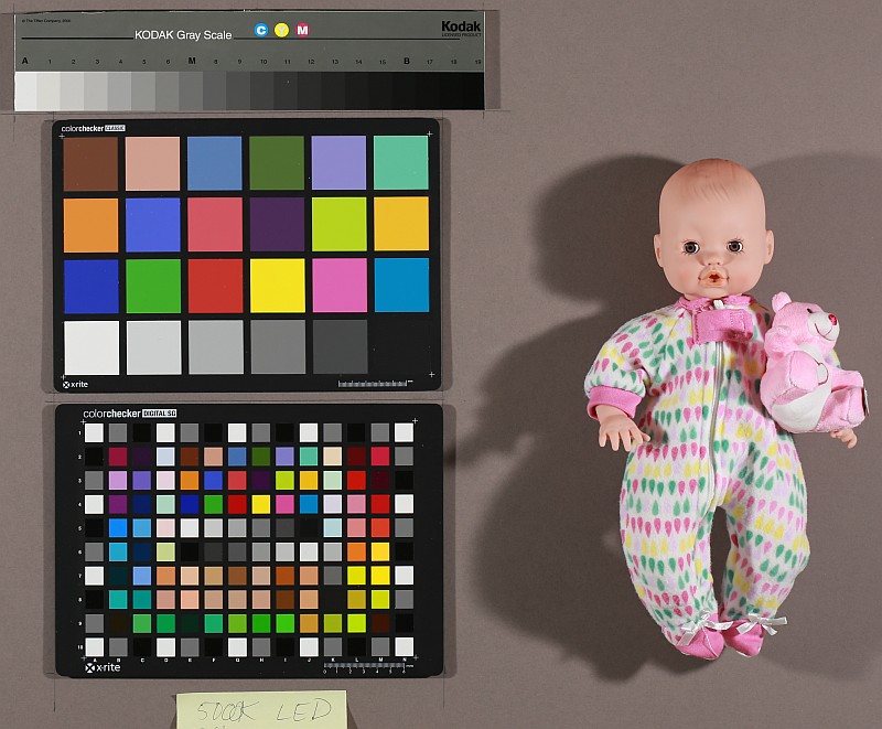 in-camera JPEG. Tonal response curveabove |
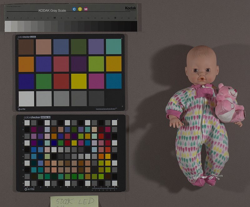 converted from CR2 raw with LibRaw. Tonal response below |
Here is the (nearly) straight-line density response for the converted CR2 raw image on the right. Though this image is typical, we have seen much larger differences between JPEG and converted raw files.
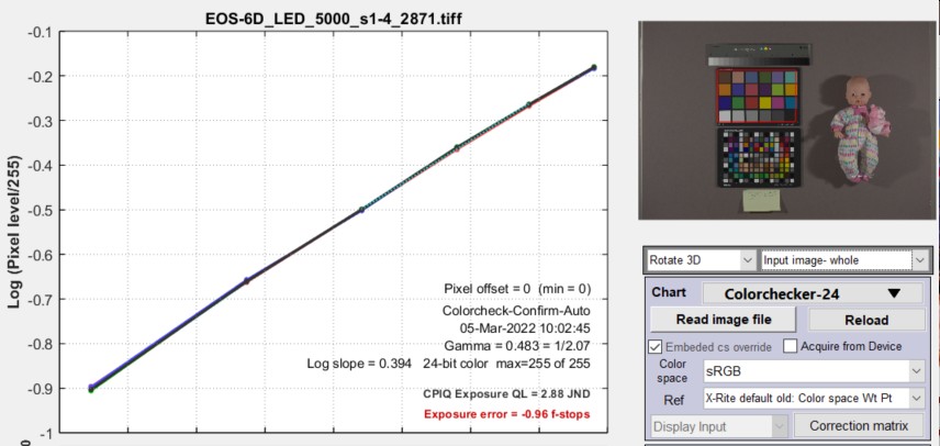 Tonal response curve from the bottom row of the Colorchecker
from the image on the right, above (converted from raw with LibRaw)
Tone mapping
Tone mapping is a form of nonuniform image processing that lightens large dark areas of images to make features more visible. It reduces global contrast (measured over large areas) while maintaining local contrast (measured over small areas) so that High Dynamic Range (HDR) images can be rendered on displays with limited dynamic range. it can usually be recognized by extremely low values of gamma (<0.25; well under the typical values around 0.45 for color space images), measured with standard grayscale charts.
Tone mapping can seriously spoil gamma and Dynamic Range measurements, especially with standard grayscale charts. The Contrast Resolution chart was designed to give good results (for the visibility of small objects) in the presence of tone mapping, which is becoming increasingly popular with HDR images.
Contrast definitions
Several definitions of contrast are used in imaging. For two luminances (or reflectances) Lmax and Lmin, which could, for example, represent two patches on a test chart,
Ratio
The most common contrast metric in Imatest documentation is Contrast ratio, \(\displaystyle C_{Ratio} = \frac{L_{max}}{L_{min}} \) It is used to specify chart contrast, for example, 4:1 for slanted-edge charts that comply with the ISO 12233 standard.
Weber
The Weber contrast \(C_{W} \) metric is based on the Weber-Fechner law on human perception. The contrast measures the difference between the high and low luminances (L) divided by the lower luminance:
\(\displaystyle C_{W} = \frac{L_{max}-L_{min}}{L_{min}} = \frac{L_{max}}{L_{min}}-1 = C_{Ratio}-1 \)Michelson
Michelson contrast \(C_{M} \) is more common in the optics field. It measures the relationship between the spread and the sum of the two luminances:
\(\displaystyle C_{M} = \frac{L_{max}-L_{min}}{L_{max}+L_{min}} \)Michelson contrast is sometimes called “modulation”, and is the basis of Modulation Transfer Function (MTF) measurements. In the SPIE Optipedia page on Modulation Transfer Function, M in equation (1.12) is none other than Michelson contrast. MTF is defined as Michelson contrast at spatial frequency f, normalized to 1 at f = 0. Amax and Amin are derived from sine waves. If sine waves are unavailable (e.g., for slanted-edges), f can be calculated from a Fourier transform (it’s 1/f for a one-dimensional edge, which has the lovely property of spatial invariance).
Michelson contrast is named after Albert Michelson, whose work on the famous Michelson-Morley experiment was a critical factor leading to Einstein’s theory of special relativity. Michelson’s life story is quite fascinating. He grew up in the wild-west mining towns of Murphy’s Camp, California and Virginia City, Nevada (there is a fictionalized Bonanza episode about his youth), and he went on to become the first American to win the Nobel prize in physics.
Logarithmic encoding
Logarithmic encoding, which has a similar intent to gamma encoding, are widely used in cinema cameras. According to Wikipedia’s Log Profile page, every camera manufacturer has its own flavor of logarithmic color space. Since they are rarely, if ever, used for still cameras, Imatest does little with them apart from calculating the log slope (n1, below). A detailed encoding equation from renderstory.com/log-color-in-depth is \(f(x) = n_1 \log(r_1 n_3+ 1) + n_2\).
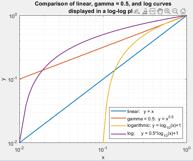
Comparison of linear, gamma (0.5) and logarithmic response curves
Comparison of linear, gamma (0.5) and logarithmic response curves
From context, this can be expressed as
\(\text{pixel level} = p = n_1 \log(\text{exposure} \times n_3+ 1) + n_2\)
Since log(0) = -∞, exposure must be greater than 1/n3 for this equation to be valid, i.e., there is a minimum exposure value (that defines a maximum dynamic range).
By comparison, the comparable (simplified) equation for gamma encoding is
\(\log(\text{pixel level}) = \log(p) = \gamma \log(\text{exposure}) \ ; \ \ \ \ \ \ p = \text{exposure}^{\gamma}\)
The primary difference is that pixel level instead of log(pixel level) is used the equation. The only thing Imatest currently does with logarithmic encoding is to display the log slope n1, shown in some tonal response plots. Imatest could do more on customer request.
Logarithmic encoding has a very different appearance from gamma encoding when viewed in log-log density plots, as shown on the right. These curves are useful for identifying logarithmic encoding. The plot below is a density response curve, made with an Imatest dynamic range chart, for a camera that produces still and video output. At this time we’re not sure it’s intentionally logarithmic, but it certainly looks it. The flattened response and steps on the left are caused by flare light.
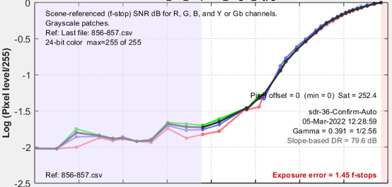
Response of an MP4 frame from a camera that produces both still and video images.
Dynamic range limitation — An issue with logarithmic spaces is that their dynamic range is strictly limited by the math since log(0) = -∞. Using the above equation and assuming that log represents log10 and n2 = 1,
\( p = \gamma \ \log_{10}(exp)+1\)
If we assume that exp is normalized to a maximum value of expmax = 1, p(expmax) = p(1) = 1. The darkest level that can be reproduced is p(expmin) = γ log10(expmin)+1 = 0.
\(\displaystyle \log_{10}(exp_{min}) = -1/\gamma \ ; \ \ \ \ exp_{min} = 10^{-1/\gamma} \)
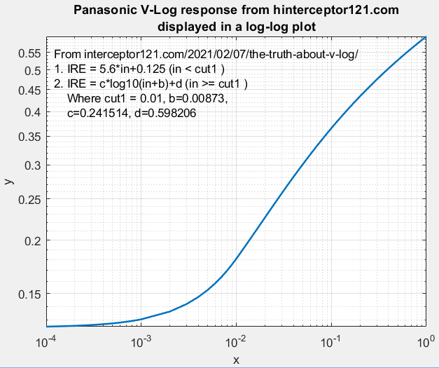
Panasonic V-LOG response
For gamma = 0.5 (shown in the plot, above right), expmin = 10-2 = 0.01, equivalent to
\(\text{Dynamic Range} = exp_{max}/exp_{min} = 1/0.01 = 100 = 40\text{dB}\)
Logarithmic response example
The truth about v-log has detailed equations for Panasonic V-LOG encoding. We programmed them because
- it’s a real example and
- it was easy.
The curve is a hybrid curve with a logarithmic section for illumination above cut1 = 0.01 and a linear section below cut1. In this respect it is somewhat similar to sRGB, which has linear and gamma sections that average to approximately gamma = 2.2.
The encoding is intended to improve dynamic range, but we have some doubts because the slope of the log-log plot is very low for the darkest regions (x < 10-3).
|
This brings us to the big question: Why is logarithmic encoding widely used in video/cinema systems? Coming from still photography, where gamma encoding is widely used (but log encoding isn’t), we are aware that gamma encoding accomplishes the same goals without the dynamic range limitation. If you have a good answer, please let us know. |
|
Misinformation warning — The Internet is full of misinformation about logarithmic color spaces. A good example is the B&H page, Understanding Log-Format Recording, which says, ” If your video—like most video—is not recorded using a log picture profile, chances are the exposure is being recorded in a linear fashion.” This is completely incorrect. The author seems to have no inkling that gamma encoding exists. Then he compounds the confusion with statements like “The problem arises with the realization that the exposure values with which we measure light are not linear. An exposure “stop” represents a doubling or halving of the actual light level, not an increase by some arbitrary linear value on a scale. You could, in fact, say exposure values are themselves logarithmic!”. Exposure Value (EV) is a relative measurement unit based on factors 2 (log2(exposure level)) that corresponds to the sensitivity of the human eye. It has nothing to do with the camera itself. For the record: Most digital sensors have a linear response, with more than 8 bits for high quality cameras (12, 14, or more bits are common). Following Analog-to-Digital conversion, most still cameras encode the image using a gamma curve. Video cameras use either gamma or log curves. As we mentioned above, this extends the effective dynamic range for gamma encoding. |
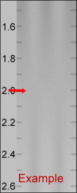
Appendix I: Monitor gamma
Monitors are not linear devices. They are designed so that Brightness is proportional to pixel level raised to the gamma power, i.e., \(\text{Brightness = (Pixel level)}^{\gamma\_display}\).
For most monitors, gamma should be close to 2.2, which is the display gamma of the most common color spaces, sRGB (the Windows and internet standard) and Adobe RGB.
|
To view the gamma chart correctly, right-click on it, copy it, then paste it into Fast Stone Image Viewer. This worked well for me on my fussy system where the main laptop monitor and my ASUS monitor (used for these tests) have different scale factors (125% and 100%, respectively). The gamma will be the value on the scale where the gray area of the chart has an even visual density. For the (blurred) example on the left, gamma = 2. Although a full monitor calibration (which requires a spectrophotometer) is recommended for serious imaging work, good results can be obtained by adjusting the monitor gamma to the correct value. We won’t discuss the process in detail, except to note that we have had good luck with Windows systems using QuickGamma. |
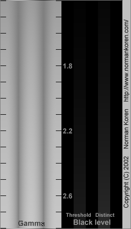 Gamma chart. Best viewed with Fast Stone image viewer. |
Appendix II: Tonal response, gamma, and related quantities
For completeness, we’ve updated and kept this table from elsewhere on the (challenging to navigate) Imatest website.
| Parameter | Definition | ||||
| Tonal response curve | The pixel response of a camera as a function of exposure. Usually expressed graphically as log pixel level vs. log exposure. | ||||
| Gamma |
Gamma is the average slope of log pixel levels as a function of log exposure for light through dark gray tones). For MTF calculations It is used to linearize the input data, i.e., to remove the gamma encoding applied by image processing so that MTF can be correctly calculated (using a Fourier transformation for slanted-edges, which requires a linear signal). Gamma defaults to 0.5 = 1/2, which is typical of digital camera color spaces, but may be affected by image processing (including camera or RAW converter settings) and by flare light. Small errors in gamma have little effect on MTF measurements (a 10% error in gamma results in a 2.5% error in MTF50 for a normal contrast target). Gamma should be set to 0.45 or 0.5 when dcraw or LibRaw is used to convert RAW images into sRGB or a gamma=2.2 (Adobe RGB) color space. It is typically around 1 for converted raw images that haven’t had a gamma curve applied. If gamma is set to less than 0.3 or greater than 0.8, the background will be changed to pink to indicate an unusual (possibly erroneous) selection. If the chart contrast is known and is ≤10:1 (medium or low contrast), you can enter the contrast in the Chart contrast (for gamma calc.) box, then check the Use for MTF (√) checkbox. Gamma will be calculated from the chart and displayed in the Edge/MTF plot. If chart contrast is not known you should measure gamma from a grayscale stepchart image. A grayscale is included in SFRplus, eSFR ISO and SFRreg Center ([ct]) charts. Gamma is calculated and displayed in the Tonal Response, Gamma/White Bal plot for these modules. Gamma can also be calculated from any grayscale stepchart by running Color/Tone Interactive, Color/Tone Auto, Colorcheck, or Stepchart. [A nominal value of gamma should be entered, even if the value of gamma derived from the chart (described above) is used to calculate MTF.]
|
||||
| Shoulder | A region of the tonal response near the highlights where the slope may roll off (be reduced) in order to avoid saturating (“bunring out”) highlights. Frequently found in pictorial images. Less common in machine vision images (medical, etc.) When a strong shoulder is present, the meaning of gamma is not clear. | ||||
Appendix III: New linearization methods introduced in Imatest 23.2
Feature summary
Imatest 23.2 introduced new options for “linearization” of slanted edge ROI image data for edge SFR analyses. The new options take the form of a dropdown on both the “Setup” (ROI selection) window and the “More Settings” window. Users can now select a “linearization method” with the following options for eSFR ISO and SFRplus analyses:
-
Input gamma value (legacy, default) – The inverse of the value entered into the “Gamma (input)” field is used to linearize the data.
-
Note: The input gamma value represents the “forward” (encoding) gamma value (typically around 0.46 = 1/2.2 for sRGB or Adobe RGB color spaces); the inverse (display gamma) is used for linearization.
-
-
Gamma calculated from chart contrast (legacy) – The value selected for the “Chart contrast” setting is used, in combination with the contrast measured from the edge ROI region, to calculate a value for gamma on a per edge ROI basis. The inverse of this gamma is used to linearize the data.
-
The gamma value is estimated from the ratio of the light and dark pixel levels P1 and P2 in the slanted-edge region (away from the edge) if the chart contrast ratio (light/dark reflectivity) has been entered (and is 10:1 or less). Starting with ,
-
Note: The calculated gamma value(s) are included in the JSON output as the field “gamma_from_chart”, on a per edge ROI basis (this is not a new output)
-
-
No linearization (new) – The data is not linearized.
-
Note: “Input gamma value” of 1 is equivalent to “No linearization”.
-
-
Linearly interpolated LUT from step chart (new, requires step chart analysis to be checked) – A linearly interpolated look-up-table (LUT), representing the inverse of the measured OECF, is calculated from the mean of the grayscale patch (step chart) ROIs and the nominal patch densities (or those from a grayscale reference file). The LUT is used to linearize the data.
-
Note: A grayscale reference file contains measured patch densities and can be loaded from the Rescharts more settings window
-
-
Gamma calculated from step chart (new, requires step chart analysis to be checked) – The mean of the grayscale patch (step chart) ROIs and the nominal patch densities (or those from a grayscale reference file) are used to calculate a value for gamma. The calculated gamma is the slope of a linear fit of the patch densities and log(grayscale patch means). The inverse of this gamma is used to linearize the data.
-
Note: A grayscale reference file contains measured patch densities and can be loaded from the Rescharts more settings window
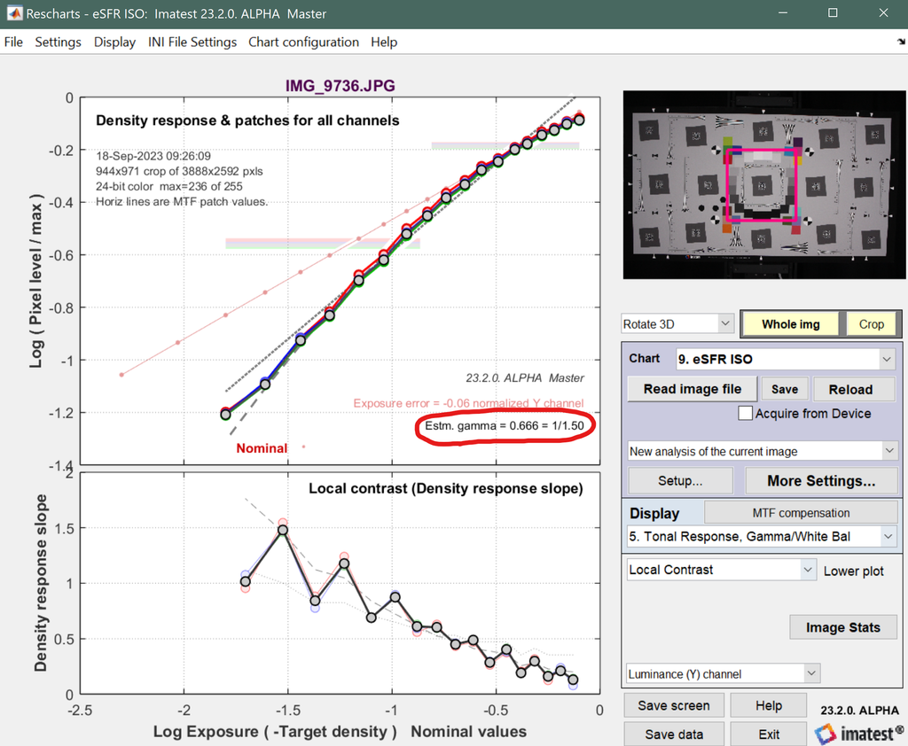
Rescharts tonal response plot showing the gamma value calculated from the step chart patches as well as the corresponding linear fit (the gamma value is the slope of the gray dotted line).
-
Note: The calculated gamma value is included in the JSON output as the field “gamma_from_stepchart” (this is not a new output)
-
Note: The range of patches used for gamma calculation is limited to those whose mean values fall within a central portion of the overall patch mean range (see the relevant section/equation above). Therefore, some darker or lighter patches may not be used for calculation of this gamma.
For edge SFR analyses that do not contain a grayscale step chart pattern, the “linearization method” options are limited to:
-
Input gamma value (legacy, default)
-
Gamma calculated from chart contrast (legacy)
-
No linearization (new, equivalent to input gamma value of 1)
 Note: The new dropdown replaces the “Use for MTF” checkbox on all relevant GUIs, which now corresponds with the “Gamma calculated from chart contrast” option in the dropdown.
The “Use for MTF” checkbox has been removed, having been replaced by the Linearization method option “Gamma calculated from chart contrast”
INI settings
A new INI field has been added for control of the new “Linearization method” setting on a per INI section (module/analysis) basis:
linearizationMethod = *valid integer*
Valid INI values are 1-5, corresponding with valid LinearizationMethod enum values.
-
1 = Input gamma value
-
2 = Gamma calculated from chart contrast
-
3 = No linearization
-
4 = Linearly interpolated LUT from step chart
-
5 = Gamma calculated from step chart
The backend logic preserves legacy setting behavior as such:
If the new linearizationMethod INI field is unset (on a per INI section basis) and the “Use for MTF” checkbox was previously checked, then the linearization method will be set to “Gamma calculated from chart contrast” (2). Otherwise, linearization method will be set to the true default “Input gamma value” (1) to preserve legacy behavior.
Outputs
The user-selected linearization method is now included as a new field in the CSV and JSON outputs, as a way of documenting the input method. The new CSV field is “Linearization method”. The new JSON field is “linearization_method”.
-
-
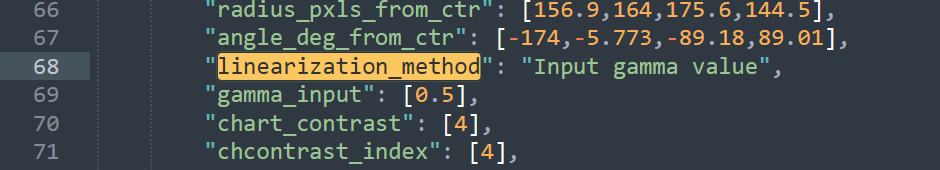
The new “linearization_method” field in the JSON output
-
-