Purple fringing – CA correction for non-tangential edges
Introduction
Chromatic aberration (CA) is one of several aberrations that degrade lens performance. (Others include coma, astigmatism, spherical aberration, and curvature of field.) It occurs because the index of refraction of glass varies with the wavelength of light, i.e., glass bends different colors by different amounts. This phenomenon is called dispersion. It appears as color fringing, most visibly on tangential edges near the boundaries of the image. It is sometimes confused with another effect, which we call pixel shift— a color channel offset that is typically uniform over the sensor and can be caused by physical misalignment of multi-chip sensors or demosaicing errors.
Minimizing chromatic aberration is one of the traditional goals of lens design. It is accomplished by combining glass elements with different dispersion properties. But it remains a problem in several lens types, most notably ultrawide lenses, long telephoto lenses, and extreme zooms. In many designs intended for digital cameras, CA is no longer a major consideration because it can be corrected in the digital domain if the correction is applied before demosaicing (as long as it’s not too extreme).
Lateral and Longitudinal CA; Tangential and radial lines
|
Measurement tips— Lateral chromatic aberration is best measured using (nearly) tangential edges near the sides or corners of the image, for example, edge B (above). It is not visible on radial edges such as A. Imatest applies a correction to edges that are not exactly tangential. Pixel shift (not CA) is best measured on near-vertical and horizontal edges near the center of the image where CA is minimum. CA cannot be measured reliably if the center of the region of interest (ROI) is less than 30% of the distance from the center to the corners. In this case, the chart will be displayed in pale colors and CA in % will be omitted. |
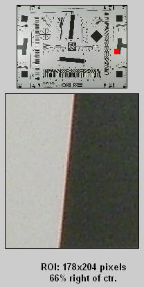
ROI for CA measurement
The two types of chromatic aberration are illustrated above.
- Longitudinal Chromatic Aberration causes different wavelengths to focus on different image planes. It cannot be measured from a single image by Imatest; it causes a degradation of MTF response— by differing amounts for different colors. It can be measured by acquiring SFRplus, eSFR ISO, or Checkerboard images at multiple distances, analyzing them as a batch, then running the resultant JSON file in the FocusField postprocessor.
- Lateral Chromatic Aberration is the color fringing that occurs because the magnification of the image differs with wavelength. It tends to be far more visible than longitudinal CA. Imatest measures Lateral CA.
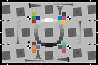
Lateral chromatic aberration is best measured on a tangential (or nearly tangential) edge near the sides or corners of an image. It is not visible on radial edges. Tangential curves and radial lines (which differ by 90 degrees) are shown in burgundy and blue in the Test chart illustration, above. Because typical Imatest SFR edges have angles in the range of 3 to 7 degrees with respect to vertical and horizontal, the best edges for measuring CA are near-vertical edges on the left and right of the image. The obsolete ISO 12233:2000 chart (shown on the right) has a very limited number of appropriate edges. One is rectangle B, above. SFRplus charts, which are available in a wide variety of sizes and media, are much better for measuring CA.
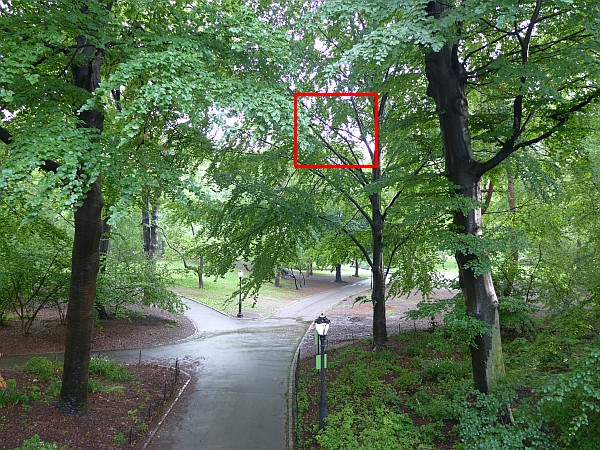
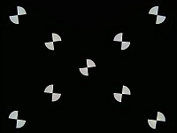
The thumbnail on the right is from a 12 megapixel compact digital camera with fairly high chromatic aberration. The selected area is shown below. Red fringing, the result of lateral CA, is clearly visible. The black-to-white edge to the right side of this rectangle has equally vivid green fringing. Imatest analyzes the edge and produces a number that indicates the severity of the lateral chromatic aberration.
Imatest chromatic aberration measurement
The average transitions for the R, G, and B color channels, calculated by Imatest SFR for the above edge, are shown in the figure below. The edges have been normalized to have asymptotic limits of 0 and 1, i.e., they are dimensionless, approaching 0 and 1 at large distances from the transition center. Note that the three edges are not simply shifted, as you might expect if the focal lengths for the three colors were slightly different. They are distorted due to demosaicing (RAW conversion), as discussed below. When Bayer RAW images (undemosaiced) are analyzed, you see simple shifts.
The visibility of the chromatic aberration is proportional to the area between the edges with highest amplitude (in this case, red) and the lowest (in this case, blue). This area can be expressed by the following integral.
\(\displaystyle CA (\text{area}) = \int \left[ Edge_{max}(x) – Edge_{min}(x) \right] dx\)
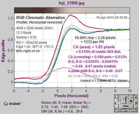 Since x has dimensions of distance in pixels and Edge is dimensionless, CA(area) has units of pixels— units of distance even though it is an area. CA defined by this equation is called the area chromatic aberration. It is displayed in magenta in the figure on the right. (CA(area) = 1.88 pixels).
The distance between the crossings (the centers of the transitions) is also shown. It is proportional to the optical CA (the actual chromatic aberration of the lens, unless it has been corrected during raw conversion), but it is less visually significant.
Chromatic Aberration figure (relatively high CA)
(shown reversed: displayed levels always increase
from left to right)
Although area in pixels is a good measure of perceptual CA, it has some shortcomings.
- It penalizes cameras with high pixel counts.
- The result depends strongly on the measurement location. The chromatic aberration in most lenses is roughly proportional to the distance from the image center.
To deal with these issues Chromatic aberration is also expressed in percentage of the distance from the image center to the Region of Interest (ROI), corrected for the angle of the ROI with respect to the center. In the above example, CA (area) = 0.110% of the distance from the image center to the ROI. The correction is described in the green box, below. This measurement gives the best overall results, since it’s relatively independent of the measurement location and the number of pixels. A table below presents rough guidelines for the severity of CA. Measurements displayed on the right of the figure are summarized in the following table.
| 10-90% rise distance (original; uncorrected) in pixels and rises per picture height (PH). |
| CA (area): Chromatic aberration area in pixels. An indicator of the visibility of CA. The area between the channels with the highest and lowest levels. In units of pixels because the x-axis is in pixels and the y-axis is normalized to 1. Explained in the page on Chromatic aberration. Measured in along the axis indicated by Profile on the upper-left. Meaning (now obsolete): Under 0.5; insignificant. 0.5-1: minor; 1-1.5: moderate; 1.5 and over: serious. |
| CA (area) as a percentage of the distance from the image center to the ROI. A better indicator than pixels (above) because it tends to be relatively consistent (at least in raw images). Equal to 100% * (area between the channels with the highest and lowest levels) / (distance from center to the ROI in pixels), corrected for the angle of the ROI. This number is relatively independent of the ROI location because CA tends to be proportional to the distance from the image center. Explained in the page on Chromatic aberration. Measured along the radial line from the image center to the edge. Meaning: Under 0.04; insignificant. 0.04-0.08: minor; 0.08-0.15: moderate; over 0.15: serious. |
|
A general equation for converting CA (in pixels) to CA (as percentage of distance from the image center to the ROI): CA (%) = 100% * CA(pixels) ⁄ (distance in pixels from the image center to the ROI) |
| CA (crossing). Chromatic aberration based on the most widely separated edge centers (positions where the edges cross 0.5). Tends to be less indicative of CA visibility than CA (area) but more indicative of the actual lens chromatic aberration. Measured two ways: (A) in pixels along the axis indicated by Profile in the upper left, and (B) in percentage of the distance from the image center to center of the ROI along the line from the image center. |
| R-G, B-G Red−Green and Blue −Green crossing shift expressed as percentage of the distance from the image center to ROI, measured along the radial line from the image center. R-G is r(Rcross)-r(Gcross), where r is radius (from the image center). |
| R-G, B-G Red−Green and Blue −Green crossing shift expressed in pixels, measured along the axis indicated by Profile in the upper left. R-G is x(R)-x(G) for horizontal profiles or y(R)-y(G) for vertical profiles, where x and y are distances along the horizontal and vertical axes, respectively. The sign may be different from the sign in the percentage measurement, depending on the measurement quadrant. |
| x-pixel shift R-G, B-G Pixel shift in the x-direction (for near-vertical edges); y-pixel shift is shown for near-horizontal edges. This is most useful for measuring pixel shift from causes other than optical chromatic aberration, and is best measured near the center of the lens. |
| Average pixel levels in the dark and light areas. Clipping can occur if they are too close to 0 or 255. |
Because Chromatic Aberration cannot be measured accurately near the image center, the chart is rendered in pale colors with the Region of Interest (ROI) is less than 30% of the distance from the center to the corner.
| Chromatic Aberration in percentage of distance from the image center |
Severity |
| 0-0.04 | Insignificant |
| 0.04-0.08 | Low. Hard to see unless you look for it. |
| 0.08-0.15 | Moderate. Somewhat visible at high print magnifications. |
| over 0.15 | Strong. Highly visible at high print magnifications. |
Imatest modules
The following Imatest modules can be used for chromatic aberration measurement. All but Dot Pattern measure Lateral Chromatic Aberration from tangential or nearly tangential slanted-edges, and also measure MTF. Some also measure optical distortion. Auto-detection slanted-edge modules are compared in www.imatest.com/docs/#sharpness.
| Module | Comments |
 SFRplus SFRplus |
Measures a great many image quality factors. The slant angles on the sides of SFPlus test charts were designed to maximize the tangential component of the vertical edges. (Contrary to rumors, we were not drunk when we designed the chart.) |
 eSFR ISO eSFR ISO |
Measures a great many image quality factors, including noise. Limited distortion measurements. |
 Checkerboard Checkerboard |
Can operate over a wide range of distances and/or Fields of View. Very accurate distortion measurements. |
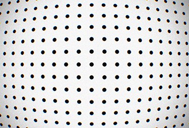 Dot Pattern Dot Pattern |
Also measures Optical Distortion (but not MTF). Corresponds to several standards. |
| SFR | Any slanted-edge, selected manually. |
 SFRreg SFRreg |
Works with ultra-wide Fields of View. Does not measure distortion. |
Demosaicing
Demosaicing is the process of converting Bayer RAW images, which have one color per pixel (RGRGRG…; GBGBGB…), to standard images, which have three colors per pixel. In the process of demosaicing, missing detail for each channel is inferred from detail in other channels. This is especially significant for Red and Blue pixels, which are half as common as Green. Demosaicing algorithms can be very mathematically sophisticated, but all of them can perform poorly in the presence of lateral CA, where detail is shifted from its expected location.
Demosaicing explains the shifted edges shown in the examples on this page. Lateral CA cannot be reliably corrected after demosaicing, but it can be corrected to near-perfection prior to demosaicing, and this is frequently done on modern cameras and camera phones. Correction coefficients can be calculated with Imatest Master, which can analyze Bayer RAW files created by converting manufacturer’s Camera RAW files. Details are in the page on RAW files.
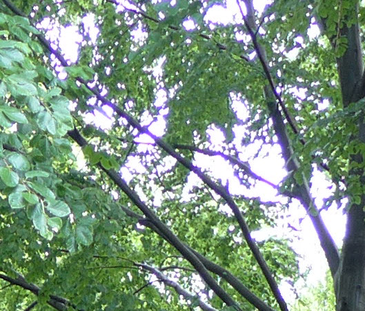
Here is an example illustrating the same region for a RAW and demosaiced file. Canon EOS-40D, 17-85mm IS lens, 50mm, f/8.
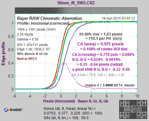 Chromatic aberration before demosaicing: easy to correct Chromatic aberration before demosaicing: easy to correctusing a different magnification for each color ((1-0.00024)x for red; 1.00062x for blue; 1 for green). |
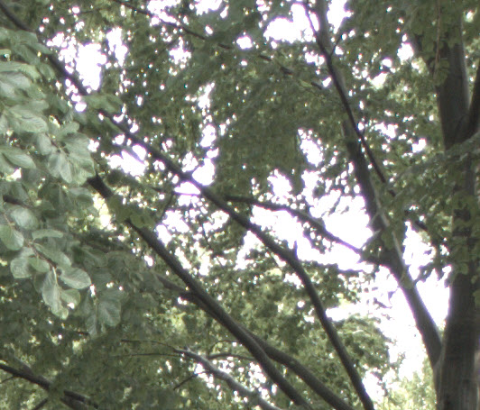
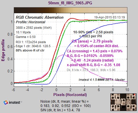 Chromatic aberration after demosaicing: difficult to correct. Chromatic aberration after demosaicing: difficult to correct.Many recent cameras (since ~2011) have CA correction built-in. |
R-G and B-G are the CA correction coefficients. They are the spacing between the Red and Green and Blue and Green crossings, respectively, expressed as percentage of the center-to-ROI distance. This measurement is relatively independent of the location of the measurement.
Chromatic Aberration correction for non-tangential edges
In Imatest, edge profiles are measured along horizontal or vertical lines. The blue line (x) on the right is an example. But chromatic aberration takes place along radial lines– lines from the center of the image to the region of measurement (shown in red on the right). Unless this line is vertical or horizontal, there will be a measurement error that must be corrected. The correction is illustrated on the right for a near-vertical edge, where the profile, and hence CA, is measured horizontally. In this illustration,
- \(x = x_1 + x_2\) is the measured chromatic aberration, along a horizontal row of pixels.
- \( C =\) the true chromatic aberration, along the radial line (angle = \(\theta\)).
- \( \phi\) is the angle of the edge relative to vertical.
\(x_1 = C \cos \theta \: ; \quad y = C \sin \theta\)
\(x_2 = y \tan \phi \) (\(x_2\) may be negative if \(\phi\) is negative.)
\(x = x_1 + x_2 = C \cos \theta + y \tan \phi = C (\cos \theta + \sin \theta \tan \phi)\)
\(\displaystyle C =\text{true chromatic aberration} = \frac{x}{\cos \theta + \sin \theta \tan \phi}\)
