Dot Pattern Target Setup

The specifics of how the dot pattern target should be prepared are flexible in that there can be an arbitrary number of dots and that size of the dots is arbitrary, subject to a few constraints. Specifically the CPIQ documents provide guidelines for preparing the dots; the dots should have a diameter sufficiently large so that the image of the dots have a diameter of no less than 10 pixels, and that for a 4/3 aspect ratio image that the size of the dot grid has no less than 20×15 dots.
Module Setup

Settings window for dot pattern analysis
The dot pattern settings window allows the selection of what kind summary figures to create after the dot pattern image has been analyzed.
Interpreting Dot Pattern Module Results
The results figures from the dot pattern analysis show the distortion and chromatic aberration of the optical system. These aberrations are summarized in several figures.
Optical and SMIA TV Distortion

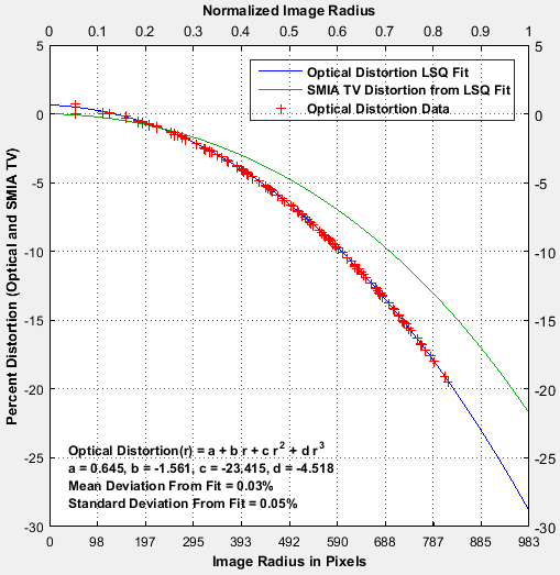
Optical distortion results.
The figure to the right summarizes the distortion of lens. The measured optical distortion as well as the best-fit optical and SMIA TV distortion curves are plotted. The distortion values are plotted against the radial coordinate as measured (in pixels) from the center of the image.
The measured optical distortion data is represented by the red crosses. A polynomial model is fit to the measured optical distortion data (using a least-squares method) and is shown in the figure as the blue curve. As a measure of the quality of the polynomial fit the figure provides the mean error and standard deviation between the measured data and the polynomial fit.
The SMIA TV distortion is plotted as the green curve. Ordinarily the SMIA TV distortion metric is taken to be a single number; the value of the green curve at the far-right of the plot. By summarizing the SMIA TV distortion as a function of image radius (rather than a single number) we gain a better understanding of the distortion aberration.
Comparison with Distortion and SFRplus modules
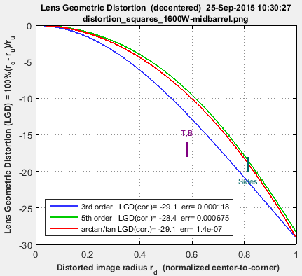
A set of images for comparing different Imatest distortion calculations can be downloaded by clicking on distortion_comparison_barrel_pin.zip. These images were created by the Test Charts module, converted to bitmaps of the same size (if needed), then equally distorted. The zip file includes barrel and pincushion-distorted images for Distortion, Dot Pattern, SFRplus, and eSFR ISO. As the Lens Geometrical Distortion figures for the three modules show, agreement is excellent. The Dot Pattern module uses the algorithm specified in the Camera Phone Image Quality (CPIQ) specification, but the other modules produce equivalent results.
Images are shown reduced. Click on the image to view full-sized.
 |
 |
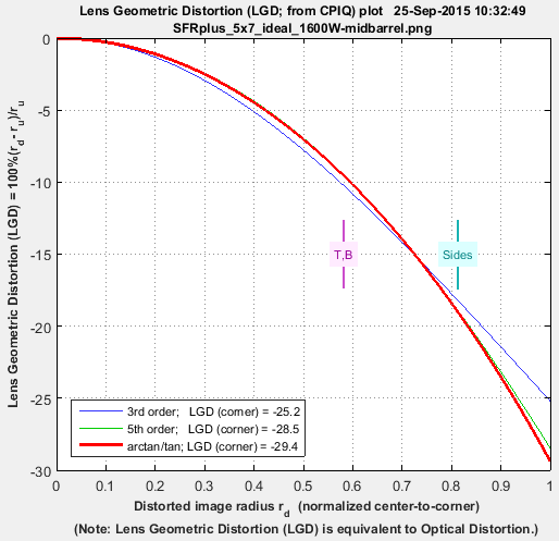 |
| Distortion module | Dot Pattern | SFRplus |
Notes: the third order calculations (Distortion and SFRplus) are less accurate than the fifth order and arctan/tan calculations (i.e., they cannot be as good a fit to the actual distortion.) The green line (SMIA TV Distortion) in the Dot Pattern figure cannot be compared with the other figures.
Grid Optical Distortion
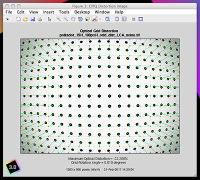
Grid distortion results.
The figure to the left summarizes the optical distortion by comparing to an ideal undistorted grid. The figure shows the image of the dot target and superimposed over the image is an undistorted Cartesian grid with thin green lines connecting the centers of the distorted dots to their undistorted Cartesian counterparts.
Radial Lateral Chromatic Aberration
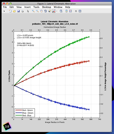
Lateral color aberration plots.
The figure to the right shows the magnitude, as a function of image radius, of the lateral chromatic aberration. The aberration is summarized by three metrics: the separation in pixels between the red and the blue channels, the red and the green channels and the green and the blue channels. Both the measured data (the crosses) as well as the best-fit polynomial models are shown.
Reported in the figure are the maximum value of the chromatic aberration expressed in both pixels and % image height (as per CPIQ).
3D Lateral Chromatic Aberration
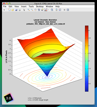
Lateral color 3D plots.
The figure on the left highlights the rotational symmetry of the lateral chromatic aberration. This figure can provide useful analysis of the asymmetry of the LCA when the 2D lateral chromatic aberration figure above shows poor agreement between the measured LCA and the best-fit polynomial approximation.