NOTE: This will be deprecated in a future release
|
Imatest 4.5+
|
|
| SFRplus also measures distortion with similar results to the Distortion module. A key advantage of SFRplus is that it can measure distortion in highly barrel-distorted (fisheye) lenses using pre-distorted charts. It can also measure Field of View (in addition to performing a great many image quality measurements). |
Distortion is one of several Imatest modules that calculate optical distortion. These modules are described in detail in Distortion: Methods and Modules.
Distortion
- measures radial lens distortion, an aberration that causes straight lines to curve,
- calculates coefficients for removing it using nonlinear optimization, and
- provides additional information on geometric distortion in digital images.
Distortion calculates the third and fifth order polynomial and arctangent/tangent distortion coefficients. These coefficients can be used to correct image distortion in the Imatest Radial Geometry module.
Lens distortion has two basic forms, barrel and pincushion, as illustrated below.
 None None |
 Barrel Barrel |
 Pincushion Pincushion |
In addition to these three, there can be “mustache” or “wave” distortion, which is barrel near the center and pincushion near the edges, or vice-versa. |
Distortion tends to be most serious in extreme wide angle, telephoto, and zoom lenses. It is most objectionable in architectural photography and photogrammetry — photography used for measurement (metrology). It can be highly visible on tangential lines near the boundaries of the image, but it is hard to see on radial lines. In a well-centered lens distortion is symmetrical about the center of the image. But lenses can be decentered due to poor manufacturing quality or shock damage.
In the simplest lens distortion model, the undistorted and distorted radii ru and rd (distances from the image center normalized to the center-to-corner distance (half-diagonal) so that r = 1 at the corner) are related by the equation,
ru = rd + k1 rd3 where k1 > 0 for barrel distortion and k1 < 0 for pincushion.
This third-order equation is one of the textbook Seidel Aberrations, which are low-order polynomial approximations to lens degradations. It only works well for small amounts of distortion. Imatest also calculates the fifth (and higher) order coefficients, which are more accurate for many complex lenses, especially those that have “wave” or “mustache” distortion, which might resemble barrel near the center of the image and pincushion near the corners (or vice-versa).
ru = rd + h1 rd3 + h2 rd5
The Wikipedia Distortion (optics) page is excellent background reading. Distortion: Methods and Modules contains a full list of Imatest-supported distortion models.
To measure distortion, you’ll need a square grid pattern or a checkerboard pattern (recommended), which you can create using Test Charts or purchase from the Imatest Store. Photograph the chart, then read the image into the Imatest Distortion module, as described below. (Reminder: Checkerboard is recommended for highly barrel distorted (“fisheye”) lenses, which cannot be analyzed with Distortion.)
Instructions
-
Test chart. You can use any chart with a square or rectangular grid or a square (checkerboard) pattern.
Checkerboards are more robust than grids, which can fail if lines are too thin or become inaccurate if lines are too thick. Results are also more accurate, especially when analyzed with the Checkerboard module.
Create the chart or purchase it from the Imatest Store.You can create your own chart using
The Screen Patterns display, shown on the right, works best with large flat screens. Click on on the right the Imatest main window, select Squares (checkerboard) or Distortion grid in the box at the bottom-center, then maximize the window. You can select the number of Horizontal and Vertical lines as well as the line width (in pixels). For best results the pattern should be square. |
 Screen Pattern for Distortion. Screen Pattern for Distortion. |
- the Distortion grid or checkerboard pattern the Imatest Test Charts module.
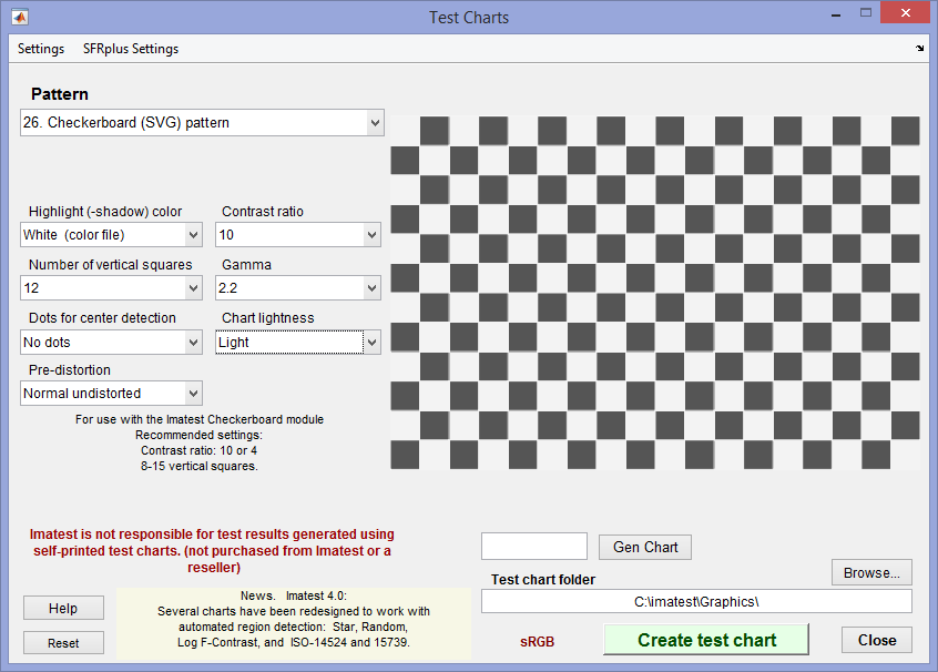 Test charts settings for SVG Checkerboard. A bitmap Checkerboard is also available.
- Recommended settings for Test Charts:
-
- Number of vertical squares. 8-16 should work for most situations. For extreme distortion, you will either need to use fewer divisions or select an ROI (i.e., crop the image).
- Contrast ratio. 4 or 10 are good numbers if MTF is to be measured (with the Checkerboard module). It MTF is not to be measured, higher contrast is OK.
- Print the test chart file. Size isn’t critical, but larger is better. (13x19 inches or larger is recommended if your printer can handle it). Matte paper is fine. Handmade charts are acceptable if they’re carefully done. The print should be made from Inkscape using the saved SVG file, not the Matlab preview.
Photograph The chart
It should be evenly lit (though lighting is less critical than with Uniformity). Lighting instructions are found in Using SFR, Part 1.
| Be careful to avoid glare “hot spots” on chart images, which can be especially troublesome with wide angle lenses. They are likely to interrupt grid lines, which will terminate Distortion analysis. To minimize glare we recommend matte surfaces. |
-
- The chart should be clean. Distortion will terminate if it mistakes spots in the image for lines. If needed, spots can be manually removed using an image editor “clone” function.
- For dark lines on a white background, set exposure compensation to overexpose by one to two f-stops so white areas are light (not middle gray) and line contrast is sufficient. This is not an issue with checkerboard charts.
- The camera should be pointed straight at the chart. (The optical axis of the lens should be normal to the chart surface.) Small amounts of tilt and perspective (keystone) distortion (convergence of lines; not a lens aberration) are tolerated, but large amounts may cause Distortion to terminate.
- The camera should be set to a low ISO speed to minimize noise. This is especially important for compact digital cameras, where noise can become severe at high ISO speeds.
Save the image. High quality JPEG format is preferred because it preserves EXIF data in a format Imatest can read. There is no need for RAW quality.
Memory problems? Because Matlab uses double precision for most math operations, each 24-bit color pixel requires 24 bytes. We recommend 8GB RAM if possible. Current versions of Imatest are all 64-bit, so memory issues are much less frequent than in the past. and also running a 64-bit version of Imatest if your operating system allows. If if that isn’t practical, click Settings (dropdown menu in the Imatest main window), Options III, and in the LARGE FILES (…, Distortion) dropdown menu, select Shrink image files 1/2x … over xx MB, where xx = 40, 80, or 20. Start at 80 and go down if needed. This shrinking (resizing) has little effect on the distortion measurements.
Launch Imatest. Click on .
Open the image file.
|
Crop the image (select the ROI) if needed using the usual clicking and dragging technique. Cropping may be helpful if horizontal or vertical lines are not entirely within the ROI (region of interest), though Imatest often works in such cases. An example is shown below in the section on Severe distortion. Click outside the the image to select the entire image. You can select either a grid pattern or a single line, which is useful in patterns such as the ISO 12233 chart, which contains two lines suitable for Distortion: one nearly vertical and one nearly horizontal (both slightly tilted). One of them is illustrated below. Make sure to leave some breathing room around the line. In selecting the crop for grid patterns (or deciding not to crop) try to choose a crop where no lines cross the crop boundaries, i.e., are partly inside and partly outside. The horizontal (well… sort of) line at the bottom right of the “Bad” image above is caused Distortion to terminate in Imatest versions earlier than 2.3.6, but is very likely to work will with 2.3.6+.
Three cropping (ROI selection) options are available by clicking Settings, Options I… in the Imatest main window. These include
| Never crop. |
| Select crop by dragging cursor. Ask to repeat crop for same sized image. |
| Select crop by dragging cursor. Do not ask to repeat crop. |
The second option (Select crop by dragging cursor. Ask to repeat crop for same sized image) is the default.
The input dialog box, shown below, appears. Title defaults to the file name; you may change it if needed. Figures can be selected in the Plot box on the right. Plot intersection points, Plot radius correction, and Display corrected image appear in Imatest Master only.
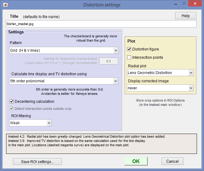 Distortion settings box
- Pattern
- For grid patterns, choose Grid.
- For lines or edges, choose Single line (some interference) or Single edge. Single line is the appropriate choice for the usable lines in the ISO-12233 pattern. “Interference” refers to extra detail that may be present near the line (lettering, etc.) This choice will work for lines near the boundaries of a grid pattern. An example from an ISO-12233 chart is shown below. We don’t recommend this setting: a grid or checkerboard will almost always produce better results.
- For checkerboard patterns (recommended), choose Squares (checkerboard). This pattern is be slightly more robust than the grid. If Squares (Checkerboard) has been selected, the Gamma for linearizing checkerboard… setting, immediately below the Pattern setting, is enabled. We recommend that you set gamma close to the encoding gamma of the camera (around 0.5 for typical color space images; 1 for raw images) to minimize waviness in edge locations.
- Calculate line display and SMIA TV Distortion using… selects the formula for plotting the corrected lines and calculating SMIA TV Distortion (by extrapolation). Useful for comparing the different algorithms. Choices are
- Decentering calculation is described below. It is optional because it takes extra time. It can only be selected for the Grid or Checkerboard patterns. It the box is unchecked, distortion is assumed to be symmetrical around the geometric center of the image.
- ROI filtering When set to Strong, this setting filters out ROIs that crashed early versions of Distortion. We recommend setting ROI filtering to Weak since many boundary conditions that formerly crashed Imatest now work well. This setting may be deprecated in the future.
- Plot area. Selects plots.
- Plot distortion figure selects the main distortion figure.
- Plot intersection points and Detect intersection points outside crop checkboxes are described below. Only for Grid and Checkerboard patterns.
- Radial plot setting is described below. Choices are None, Delta-r, or Lens Geometric Distortion.
- Display corrected image displays the corrected image calculated with the algorithm selected in Calculate line display (3rd order, 5th orcer, or arctan/tan) using, above. It is most valuable for highly distorted lenses where the input image has been cropped. Choices are never, crop only (the default), and always. An example is shown below in the section on Severe distortion.
Click . The calculations are performed, and the results figure(s) described in Results appears. You can zoom in by clicking on (and highlighting) the magnifier icon ![]() , then clicking on portions of the image of interest, as shown below. The detected points on the image are shown as red squares. The straightened line is drawn in magenta. Double-clicking
, then clicking on portions of the image of interest, as shown below. The detected points on the image are shown as red squares. The straightened line is drawn in magenta. Double-clicking ![]() restores the entire image.
restores the entire image.

An enlarged portion of the results figure.
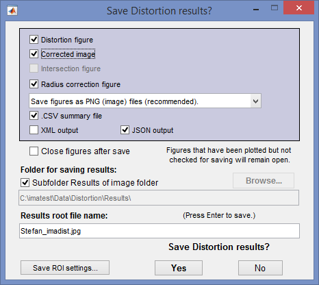 Save results dialog box
When the calculations are complete the Save dialog box appears. The default directory is subfolder Results in the data file folder. You can change to another existing folder if needed.The selections are saved between runs. You can examine the output figures before you check or uncheck the boxes. Select the items you wish to save, then click or . File names (where filename is the input file name):
[filename]_distortion.png
[filename]_corrected.png (only if displayed) [filename]_intersections.png [filename]_radius_corr.png [filename]_summary.csv [filename]_summary.csv [filename].xmlThe root file name ([filename], above) defaults to the image file name, but can be changed using the Results root file name box. Be sure to press enter. Checking Close figures after save is recommended for preventing a buildup of figures (which slows down most systems) in batch runs.
The CSV and XML files contain EXIF data, which is image file metadata that contains important camera, lens, and exposure settings. \To read detailed EXIF data from all image file formats, we recommend downloading, installing, and selecting Phil Harvey’s ExifTool, as described here.
Results: Main figure
An example of Distortion output is shown below for the Sigma 18-125 mm f/3.5-5.6 DC lens (designed for APS-C-sized sensors. The Sigma is an excellent bargain, except for its rather unreliable autofocus, but it works beautifully on manual. The autofocus problem is plainly visible when working with the distortion chart.
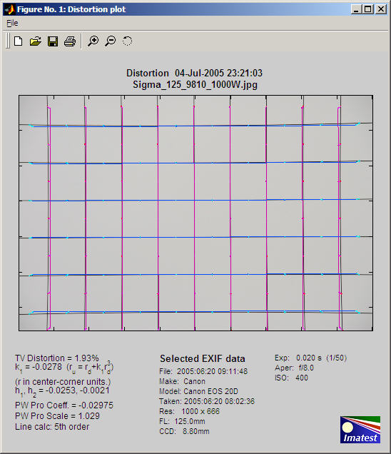
Main figure showing modest pincushion distortion
The Sigma has modest amounts of pincushion distortion at 125 mm and barrel distortion at 18mm, its widest angle setting. Corrected vertical lines are deep magenta; horizontal lines are blue. The following results are displayed on the left below the image.
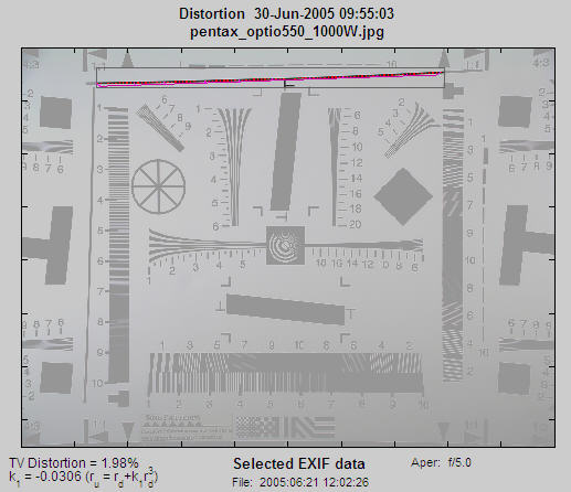
SMIA TV Distortion
-
SMIA* TV Distortionfrom the SMIA specification, §5.20. Referring to the image on the right,
SMIA TV Distortion = 100( A-B )/B ; A = ( A1+A2 )/2
The box on the right is described in the SMIA spec as “nearly filling” the image. Since the test chart grid may not do this, Distortion uses a simulated box whose height is 98% that of the image. Note that the sign is opposite of k1 and p1. SMIA TV Distortion > 0 is pincushion; < 0 is barrel.
[*SMIA is the now-defunct “Standard for Mobile Imaging Architecture”, started by Nokia and STMicroelectronics in 2004.]Algorithm: SMIA TV Distortion is not actually calculated from the upper and lower horizontal lines in the chart, whose locations can vary considerably for different images. Instead it is calculated from the distortion coefficients: 3rd order (k1) prior to Imatest 3.7; 5th order (h1 and h2; slightly more accurate) for 3.7-3.9, and the setting used for the line display (5th order recommended) for 3.10+. The coefficients are used to create virtual horizontal lines (by extrapolation) located 1% of the image height below the top and above the bottom of the image.
|
SMIA TV distortion is twice as large (2X) as traditional TV distortion. The traditional definition, shown on the right, has been adapted from the publication “Optical Terms,” published by Fujinon. The same definition appears in “Measurement and analysis of the performance of film and television camera lenses” published by the European Broadcasting Union (EBU). At Imatest we prefer the SMIA definition, which has been widely adopted in the mobile imaging industry, because it is self-consistent. In the traditional definition, TV distortion is the change (Δ) of the center-to-top distance divided by by the bottom-to-top distance. In the SMIA definition, both A and B are bottom-to-top distances. Traditional TV distortion is likely to be included in an upcoming ISO standard. When this happens we’ll offer a choice (a checkbox). |
Although any number in this list can be used as a summary measure of distortion, SMIA TV distortion is a good choice because it’s easy to visualize.
- Coefficient k1 from the equation, ru = rd + k1 rd3 where r is normalized to the center-to-corner distance. k1 = 0 for no distortion; k1 < 0 for pincushion distortion; k1 > 0 for barrel distortion.
- Coefficients h1 and h2 from the fifth-order equation, ru = rd + h1 rd3 + h2 rd5. The selected area must contain at least five horizontal and vertical lines.
- The Lens Distortion correction coefficient and scale factor for Picture Window Pro. The sign is the same as k1. The scale factor is the value that includes as much as possible of the original image without including areas outside the image. It is less than 1 for barrel distortion and greater than 1 for pincushion.
- The calculation used for plotting the corrected lines. Selected in the input dialog box. 3rd order, 5th order, and Picture Window Pro are the choices.
Picture Window Pro uses a tangent/arctangent model of distortion, which works well for a variety of lenses, including fisheyes.
ru = tan(10 p1 rd )/ (10 p1 ) ; k1 > 0 (barrel distortion)
ru = tan-1(10 p1 rd )/ (10 p1 ) ; k1 < 0 (pincushion distortion)
Where p1 is the correction coefficient. Using Taylor series, we can show that it is similar to the third-order model,
tan(x) = x + x3/3 +2x5/15 + … ; tan-1(x) = x – x3/3 + x5/5 – … ( x2 < 1) ;
ru = x + 100 p12x3/3 + … (barrel); ru = x – 100 p12x3/3 + … (pincushion) ,
k1 ≈ sign( p1)*100 p12/3 for small values of k1 and p1. k1 and p1 diverge for large values.
The plot includes arrows that illustrate the change in radius when distortion is corrected. Distortion was too low on the above plot to make the arrows visible. They are illustrated in the plot below for a large amount of simulated barrel distortion. You can try different line display calculations to see the difference.
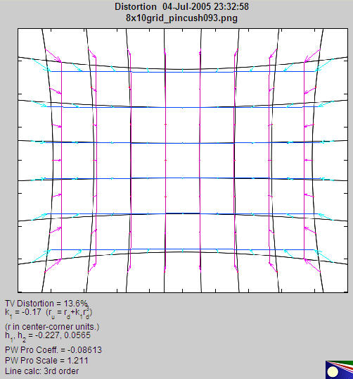
Main figure with extreme (simulated) pincushion distortion, illustrating arrows.
Here is an example of results from an ISO 12233 test pattern, which contains two lines suitable for measuring distortion. They work but they’re not ideal: they would be better if they were thinner and closer to the image boundaries. This camera has a modest amount of pincushion distortion. A zoom of a portion of the selected area is shown above.
Results: Decentering (not in Studio)
Distortion is normally centered around the geometric center of the image, but it may be decentered due to poor lens manufacturing quality or shock (i.e., dropping the lens). Decentering can appear as a shift in the center of distortion symmetry or as asymmetrical MTF (sharpness) measurements in SFR. Distortion calculates decentering if Decentering calculation is checked in the Input dialog box and |k1| > 0.01. (k1 is the third-order coefficient.) If |k1| is smaller, distortion is insignificant (and difficult to see); hence decentering has no meaning.
Decentering is reported by the radius (in units of the distance from the image center to the corner) and angle in degrees of the center of distortion symmetry. It is illustrated in the simulated pattern below. The geometrical center of the image is indicated by a pale blue +. The center of the decentered distortion is indicated by bold red X.

Results showing centering (+ for image; X for distortion center)
Severe distortion: Corrected image figure
Although we recommend SFRplus with pre-distorted charts for analyzing images from severely distorted (fisheye) lenses, the Distortion module can be used with cropping to facilitate the detection of vertical and horizontal lines. (See good/bad images, above.) The figure below was captured with an inexpensive fisheye lens. The crop area, shown in the middle, is displayed with full contrast; the area outside the crop has reduced contrast.

Severely distorted image
This figure does not show the corrected grid image outside the crop. The different correction formulas (3rd order polynomial, 5th order polynomial, or tangent/arctangent) can only be compared inside the crop area, where optimum coefficients have been calculated. They don’t look very different in this region. 3rd order is generally not recommended for strongly distorted images.
If Display corrected image in the input dialog box (Imatest Master only) is set to crop only or Always, the corrected image (shown below) is displayed. (The extreme corners are omitted for large amounts of barrel distortion). This figure is not perfect. It is calculated using a simple, fast algorithm that omits some pixels on the left and right. A semicircular “fingerprint” pattern” appears in their place. But is good enough to clearly illustrate the performance of the correction algorithm. (Another option, always – interpolated (SLOW!), produces a fine image without any gaps, but is too slow to be recommended.)
In this case, some residual barrel distortion is visible in vertical grid lines on the left and right and some residual pincushion distortion is visible in the horizontal grid lines on the top and bottom. The average correction is quite good. The tangent/arctangent algorithm (used in Picture Window Pro) gives slightly better results for this image than the 5th order polynomial (which is normally most accurate), and much better than the 3rd order polynomial.

This image has some perspective distortion: vertical convergence of lines. This results from the way the camera was pointed when the image was captured. It is not a lens aberration.
Results: Intersection figure (not in Studio)
Checking Plot intersection points in the input dialog box displays a second figure that contains intersection points (line crossings) designated by “+,” “T,” or “L.” “+” intersection points are inside the pattern; “T” points are on the boundaries (top, bottom, and sides), and “L” points are on the corners.
Intersection figure
The image should be cropped so that only “+” intersection points (line crossings) are present inside the crop. Imatest doesn’t like boundaries with “T” or “L” patterns inside the crop. To detect such patterns, they must be outside the crop (as shown above) and Detect points outside crop must be checked in the input dialog box. These points are not used in the for calculating distortion coefficients.
The mean horizontal and vertical line spacings (ΔX and ΔY) are shown beneath the plot and in the optional CSV and XML files, along with the spacing ratios (the distortion aspect ratios), ΔY ⁄ ΔX and ΔX ⁄ ΔY.
If the image contains letters or material unrelated to the the pattern, it should be edited out using an image editor. Picture Window Pro has a particularly convenient means of creating a rectangular mask for this purpose.
The (x,y) coordinates of the displayed points are included in the optional .CSV and XML output files. These coordinates can be used for further analysis of geometric distortion.
Thanks is due to Karl-Magnus Drake of the National Archives of Sweden for suggesting this figure.
Results: Radial Distortion plot (not in Studio)
|
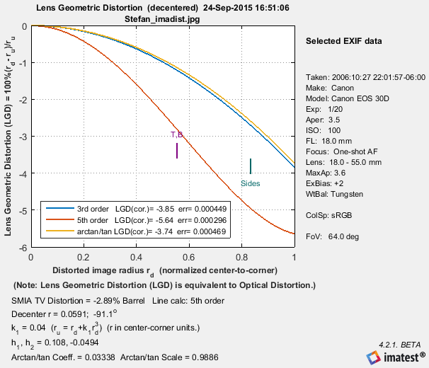
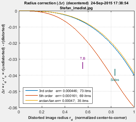
Checking either Delta-r or Lens Geometric Distortion in the Radial plot dropdown menu in the Settings window displays a detailed radial distortion plot that can be useful for analyzing images like the one on the right, which has “wave” or “mustache” distortion— barrel near the center but tending towards pincushion near the corners. The figure shows either
Δr = r(undistorted) – r(distorted) = rd – ru
LGD = 100% ( rd – ru)/ru LGD is defined in the CPIQ Phase 2 specification, and is equivalent to optical distortion as defined by Edmund Optics. |
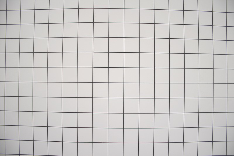 Image showing complex (“wave”) distortion: barrel near Image showing complex (“wave”) distortion: barrel near
center; pincushion near corners. Click to display |
|
The bold solid lines show Δr or LGD for correction formulas: ru = rd + k1 rd3 (3rd order; blue); ru = rd + h1 rd3 + h2 rd5 (5th order; green); or the arctan/tan equations (red). With these equations |Δr| often increases as a function of r(distorted), i.e., it tends to be largest near the image corners. The legend includes the optimization error (err, described in the Algorithm). Here is the Lens Geometric Distortion (LGD) plot. The 5th order calculation has the lowest error, which is expected because only 5th order can fit wave distortion. (The others are only good for simple barrel or pincushion.) |
 |
|
And here is the corresponding Δr plot. The Radial Distortion plot in SFRplus and Checkerboard can display two additional results— r undistorted (ru), or d(LGD)/d(ru). |
 |
Comparison with other modules
Distortion results are very close to results from other modules. There is a detailed comparison in Distortion: Methods and Modules.
|
Curvature ( d 2ru /drd2 ) and Distortion (Curvature/r) are plotted as dashed ( – – – ) and bold solid —— lines, respectively, in the lower plot.
Interpretation:
Positive Distortion (and Curvature) represents local barrel distortion;
Negative represents local pincushion distortion.
In the example above, distortion goes from barrel to pincushion around rd = 0.8 (the diameter at the sides of the image). This is visible near the corners, where the (barrel) curved lines straighten out.
The blue lines (3rd order equation) are the simplest but least accurate approximation to distortion. The 5th order equation (red lines), which has two parameters (h1 and h2 ), is more accurate. If the 3rd and 5th order curves are close, the 3rd order curve is sufficient. In the above example, which is not typically, they are very different; the third order equation is completely inadequate. The arctan/tan equation is also characterized by a single parameter. It behaves differently from the 3rd order equation for large Δr.
The 3rd order distortion value in the figure is a constant solid blue blue equal to 6 k1 .
Links
Distortion by Paul van Walree, who also has excellent descriptions of several of the lens (Seidel) aberrations and other sources of optical degradation.
Optical Metrology Center A UK consulting firm specializing in photographic metrology. They have a large collection of interesting technical papers emphasizing distortion and 3D applications, for example, Extracting high precision information from CCD images.
PTlens is an excellent program for correcting distortion. It uses the equation from Correcting Barrel Distortion by Helmut Dersch, creator of Panorama Tools, who states,
Photogrammetry is the science of making geometrical measurements from images. George Karras has sent me some interesting links with material relevant to Imatest development: http://www.vision.caltech.edu/bouguetj/calib_doc/ | http://nickerson.icomos.org/asrix/index.html.
The correcting function is a third order polynomial. It relates the distance of a pixel from the center of the source image (rsrc) to the corresponding distance in the corrected image (rdest) :
rsrc = ( a * rdest3 + b * rdest2 + c * rdest + d ) * rdest
The parameter d describes the linear scaling of the image. Using d=1, and a=b=c=0 leaves the image as it is. Choosing other d-values scales the image by that amount. a,b and c distort the image. Using negative values shifts distant points away from the center. This counteracts barrel distortion… The internal unit used for rsrc and rdest is the smaller of the two image lengths divided by 2.
This equation drives me nuts! rsrc and rdest are reversed from the equations on this page; it only goes up to fourth power (when you include rdest outside the parentheses; third power if you don’t); and it has even order terms (a and c) when the theory implies that distortion can be modeled with odd terms only. Give me a higher order term (h * rdest4 ) and dump a * rdest3 and c * rdest. But nonetheless it works pretty well.
|
Modeling distortion of super-wide-angle lenses for architectural and archaeological applications by G. E. Karras, G. Mountrakis, P. Patias, E. Pets
