Lens (optical) distortion is an aberration that causes straight lines to curve near the edges of images. It can be troublesome for architectural photography and photogrammetry (measurements derived from images). The simplest approximation is the 3rd order equation, ru = rd + krd3 where rd is the distorted and ru is the undistorted radius. Depending on the sign of k, it can be either “barrel” (shown on the right) or “pincushion.” A mixture known as “mustache” distortion may occur for complex lenses which are better described by a 5th order approximation (ru = rd+ h1rd3+ h2rd5) .
Lens distortion and coefficients for correcting it are calculated in the Checkerboard module, which calculates 3rd order, 5th order and tangent/arctangent distortion model along with sharpness and several other factors, Dot Pattern performs CPIQ-compliant distortion measurement. SFRplus measure distortion with almost as much detail as checkerboard. SFRplus distortion results are in the Image, Geometry, Distortion, FoV and Radial distortion plots. eSFR ISO measures distortion with slightly less precision than SFRplus.
Distortion is worst in wide angle, telephoto, and zoom lenses. It often worse for close-up images than for images at a distance. It can be easily corrected in software. For more details see Distortion: Methods and Modules.
See Also:
- Distortion: Methods and Modules
- Picture Window Pro and PTLens have tools for removing it.
Related standards:
Distortion Modules and Methods
This page describes Imatest’s distortion calculations, comparing the different distortion formulas and modules.
Distortion formulas – Modules – TV Distotion and Field of View – Image, Geometry, Distortion, FoV display
Radial distortion plot – Distortion Contour plot – Compare results – Links
Lens distortion has two basic forms, barrel and pincushion, as illustrated below.
 None None |
 Barrel Barrel |
 Pincushion Pincushion |
In addition to these three, there can be “mustache” or “wave” distortion, which is barrel near the center and pincushion near the edges, or vice-versa. |
Distortion formulas
In the equations which apply to several modules, rd is the distorted (measured) radius normalized to the center-to-corner distance. ru is the undistorted radius. r is normalized to the center-to-corner distance.
| N* | Distortion model | Standard | Division (Power is one less than standard model) |
Notes |
| 1 | 3rd order polynomial | \(r_u = r_d + k_1 r_d^3\) | \(r_u = r_d / (1 + k_1 r_d^2)\) | [1][A] |
| 2 | 5th order polynomial | \(r_u = r_d + k_1 r_d^3 + k_2 r_d^5\) | \(r_u = r_d / (1 + k_1 r_d^2 + k_2 r_d^4)\) | [2] |
| 3 | Tangent (for barrel distortion) | \(r_u = \tan(10 p_1 r_d )/(10 p_1 ) ;\;\; p_1 > 0\) | [1][A] | |
| 3 | Arctangent (for pincushion distortion) | \(r_u = \arctan(10 p_1 r_d )/(10 p_1 ) ;\;\; p_1 < 0\) | [1][A] | |
| 4 | The best of the above choices (3rd order, 5th order, and arctangent/tangent) | |||
| 6 | 5th order ALL polynomial | \(r_u = r_d + k_1 r_d^2 + k_2 r_d^3 + k_3 r_d^4 + k_4 r_d^5\) | \(r_u = r_d / (1 + k_1 r_d + k_2 r_d^2 + k_3 r_d^3 + k_4 r_d^4)\) | [3] |
| 7 | The best of 7th order polynomial and arctangent/tangent: Available in Checkerboard. |
|||
| 8 | 7th order polynomial | \(r_u = r_d + k_1 r_d^3 + k_2 r_d^5 + k_3 r_d^7\) | \(r_u = r_d / (1 + k_1 r_d^2 + k_2 r_d^4 + k_3 r_d^6)\) | [4] |
| 9 | 7th order ALL polynomial | \(r_u = r_d + \sum_{i=2}^7 k_{i-1} r_d^i\) | \(r_u = r_d /( \sum_{i=1}^6 k_i r_d^i)\) | [4] |
| 10 | 9th order polynomial | \(r_u = r_d + k_1 r_d^3 + k_2 r_d^5 + k_3 r_d^7 + k_4 r_d^9\) | \(r_u = r_d / (1 + k_1 r_d^2 + k_2 r_d^4 + k_3 r_d^6 + k_4 r_d^8)\) | [4] |
| 11 | 11th order polynomial | \(r_u = r_d + \sum_{i=1}^5 k_i r_d^{2i+1}\) | \(r_u = r_d / (r_d + \sum_{i=1}^5 k_i r_d^{2i})\) | [4] |
Notes: [1] All modules. [2] All except eSFR ISO. [3] Checkerboard and SFRplus. [4] Checkerboard-only.
[A] arctan/tan and 3rd order models are inadequate for measuring wave (mustache) distortion. A minimum of a 5th order polynomial is required.
 |
 |
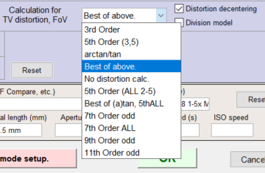
*N is the index of the distortion calculation dropdown menu in More settings. N = fovcalc in ini files for the above modules. It is displayed by the INI File Monitor. N = fovcalc = 5 is for no distortion (no FoV) calculation. 4 is for the best of 1-3. 7 is for the best of 3, 6.
- The third-order equation is one of the textbook Seidel Aberrations, which are low-order polynomial approximations to lens degradations. It only works well for small amounts of distortion
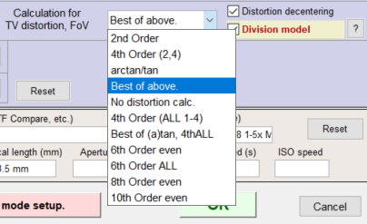
- The Division distortion model (for polynomials) appears to be slightly more accurate than the standard model for the same number of coefficients. When chosen, nth order (odd) polynomials are replaced by (n-1)th order (even) polynomials, as shown above.
- Fifth (and higher) order coefficients produce more accurate results, especially for “wave” or “mustache” distortion, which might resemble barrel near the center of the image and pincushion near the corners (or vice-versa).
- The two settings with ALL polynomial coefficients (5th order ALL and 7th order ALL) use all coefficients up to the maximum instead of alternate coefficients (odd or even-only, depending on how the model). We have not observed much advantage to these settings.
- Higher order polynomials (7th order or higher; available only with Checkerboard) should be used with great care because results can become unstable, especially at the outer parts of the image. The image used to calculate the coefficients should have valid corner points near the edge of the image and there should be sufficient rows or columns.
Modules
| Module | Comments | Advantages | Disadvantages |
| Checkerboard | Extremely accurate. Recommended for new projects. | Fast (after pattern detection). Extremely accurate (good enough for camera calibration). Distortion center calculation is very fast and should always be selected. Also calculates MTF and LCA. Framing and alignment are not critical. Wide range of working distances. Works well with strongly barrel-distorted images. | Works only with checkerboard pattern. Checkerboard detection may be slow, but remaining calculations are fast. |
| Dot pattern | Based on CPIQ Part 2 document. | CIPQ and ISO-compliant. Also measures Lateral Chromatic Aberration (LCA). | Intolerant to misalignment. Somewhat slow. We may add the algorithms used in Checkerboard, which are more flexible. |
| SFRplus |
A highly versatile module with many image quality factor measurements | Fast and moderately accurate. Also calculates MTF, Lateral Chromatic Aberration, color and tonal response. Works with pre-distorted charts (useful with strongly barrel-distorted images). See SFRplus Distortion and Field of View measurements for more detail, especially about using pre-distorted charts. | Slightly less accurate than Checkerboard. The image should have a small amount of white space above and below the top and bottom bars. This limits the range of working distances. |
| Distortion Not recommended for new projects. |
Imatest’s original (legacy) module for calculating distortion. May be deprecated in a future release. | Works with grid patterns, lines and edges, as well as checkerboard patterns. | Often fails with strongly barrel-distorted images. Less accurate than Checkerboard. Only measures distortion (no MTF, etc.). Grid patterns can be difficult to work with because grid lines can be lost if they’re too thin, and precision is lost if they’re too thick. |
| eSFR ISO | Limited distortion calculation. No distortion center. | Distortion is calculated along with other results. | Limited distortion formulas. Does not work with higher-order polynomials. |
TV distortion and Field of view
SMIA* TV Distortion is calculated from the distortion model equation (and the Distortion parameters for pre-distorted charts). [*SMIA is the now-defunct “Standard for Mobile Imaging Architecture”, started by Nokia and STMicroelectronics in 2004.]
 TV Distortion from the SMIA specification, §5.20. Referring to the image on the right,
SMIA TV Distortion = 100( A-B )/B ; A = ( A1+A2 )/2
The box on the right is described in the SMIA spec as “nearly filling” the image. Since the test chart grid may not do this, Distortion uses a simulated box whose height is 98% that of the image. Note that the sign is opposite of k1 and p1. SMIA TV Distortion > 0 is pincushion; < 0 is barrel.
Algorithm: SMIA TV Distortion is not actually calculated from the upper and lower bars, whose locations can vary considerably in different images. Instead it is calculated from the distortion coefficients using the selected equation, and using virtual horizontal lines located 1% of the image height below the top and above the bottom of the image.
|
SMIA TV distortion is twice as large (2X) as traditional TV distortion, now included in several standards. The traditional definition, shown on the right, has been adapted from the publication “Optical Terms,” published by Fujinon. The same definition appears in “Measurement and analysis of the performance of film and television camera lenses” published by the European Broadcasting Union (EBU). |
 SMIA vs. traditional (ISO) TV distortion
At Imatest we have traditionally used the SMIA definition, which has been widely adopted in the mobile imaging industry, because it is self-consistent. In the traditional definition, TV distortion is the change (Δ) of the center-to-top distance divided by by the bottom-to-top distance. In the SMIA definition, both A and B are bottom-to-top distances.
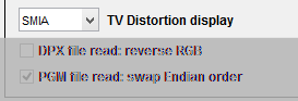 Imatest 5.1+ allows you to select between traditional TV distortion (now a part of several ISO standards, including ISO 16505) and SMIA TV distortion. You can make the selection on the left side of the Options II window (button on the lower-right of the Imatest main window). The selection affects only graphic displays (ISO TV distortion = SMIA TV distortion ⁄ 2). Both results are included in CSV and JSON results (for all modules that calculate distortion).
Field of view (FoV) is calculated for SFRplus, Checkerboard, and eSFR ISO by applying the distortion model equation to the top, side, and diagonal (always r = 1) of the image. In order to calculate FoV in units of distance (cm) a chart geometrical distance has to be entered into the Rescharts More settings window.
| Module | Value |
| SFRplus | Bar-to-bar chart height in cm |
| Checkerboard | Square spacing (cm) |
| eSFR ISO | Reg. mark vertical spacing cm |
If the Lens-to-chart distance (in cm) is entered, angular FoV will also be calculated.
Image, Geometry, Distortion, FoV display
An image display is available in most modules that calculate distortion. In Rescharts it contains a large amount of information (not all distortion-related). Here is an example showing arrows and lines to the corrected image, available for Checkerboard-only. (The arrows & lines can be turned on or off in the More settings window.)
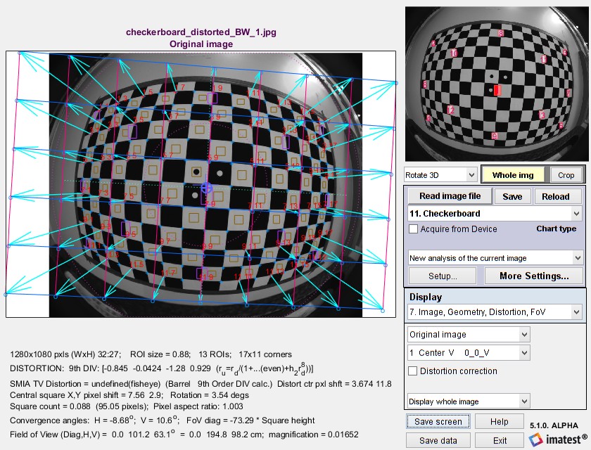 Image, Geometry display showing arrows and corrected image locations
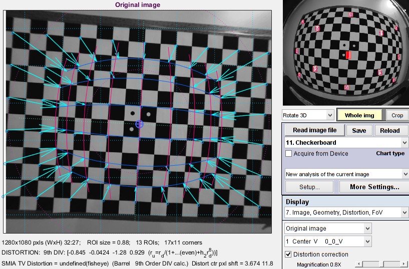
Corrected image showing arrows to original image
Click on the image to view full-sized.
Here is an example of the corrected image, also showing arrows and lines.
This display contains
- Dimensions andROI information (for MTF calculations)
- Distortion coefficients (9th order division model here)
- SMIA TV distortion
- Distortion center shift (in pixels)
- Image (central square) shift
- Field of View (Diagonal, Horizontal, and Vertical; degrees and cm if appropriate settings have been entered)
- Convergence angles (perspective distortion)
Radial distortion plot
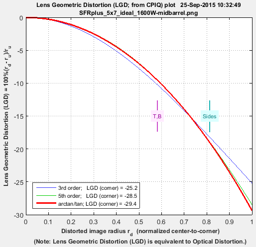
The radial distortion plot is available in modules that calculate distortion. This plot has four display options: 1. Delta-r, or 2. Lens Geometric Distortion (LGD), 3. r undistorted (ru), or d(LGD)/d(rd). LGD is shown below.
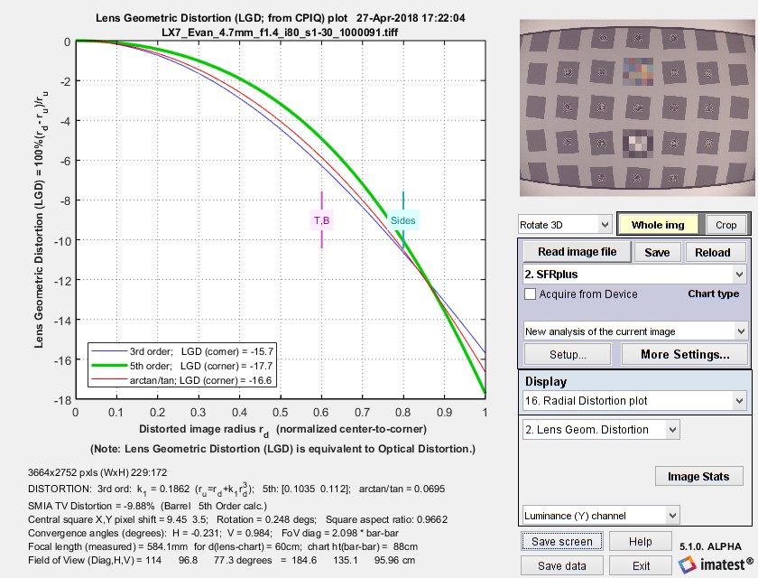 SFRplus Radial Distortion plot showing Lens Geometric Distortion 100% ( rd – ru)/ru
The display options are
- the change in radius Δr (normalized to the center-to-corner distance, i.e., the half-diagonal) as a function of the distorted (input) radius rd.
Δr = r(distorted) – r(undistorted) = rd – ru - Lens Geometric Distortion (LGD), which is included in the CPIQ Phase 2 specification, and is equivalent to Optical Distortion (defined by Edmund Optics).
LGD = 100% ( rd – ru)/ru - Undistorted radius, ru
- Curvature d(LGD)/d(rd). This curvature (new in Imatest 5.0) may be useful for determining the visual degradation caused by distortion, which is likely to be proportional to the maximum-minimum values. A change in sign may be a better indicator of mustache (wave) distortion than a change in 5th order polynomial sign (which isn’t always calculated).
The solid lines show results for correction formulas: ru = rd + k1 rd3 (3rd order polynomial; blue); ru = rd + h1 rd3 + h2 rd5 (5th order ploynomial; green); or the arctan/tan equations (red). The best fit (5th order in this case) is shown in bold. With these equations |Δr| often increases as a function of r(distorted), i.e., it tends to be largest near the image corners. The selected value (or the one with the least error, err) is shown in boldface.
Distortion Contour plot – Checkerboard-only
New in 2021.2. Described in Rescharts Slanted-Edge modules Part 4: Distortion contour plot.
Comparison of results for different modules
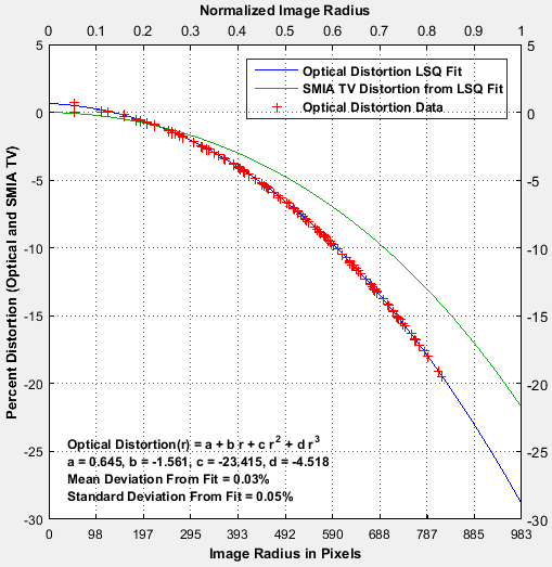
A set of images for comparing different Imatest distortion calculations can be downloaded by clicking on distortion_comparison_barrel_pin.zip. These images were created by the Test Charts module, converted to bitmaps of equal size, then equally distorted. The zip file includes barrel and pincushion-distorted images for Distortion, Checkerboard, Dot Pattern, SFRplus, and eSFR ISO. As the Lens Geometrical Distortion figures for the modules show, agreement is excellent. The Dot Pattern module uses the algorithm specified in the Camera Phone Image Quality (CPIQ) specification, but the other modules produce equivalent results.
Images are shown reduced. Click on the image to view full-sized.
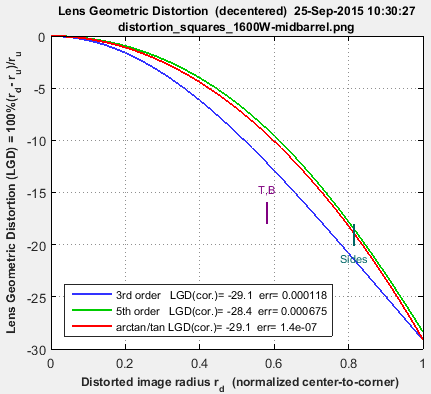 |
 |
 |
| Distortion module | Dot Pattern | SFRplus |
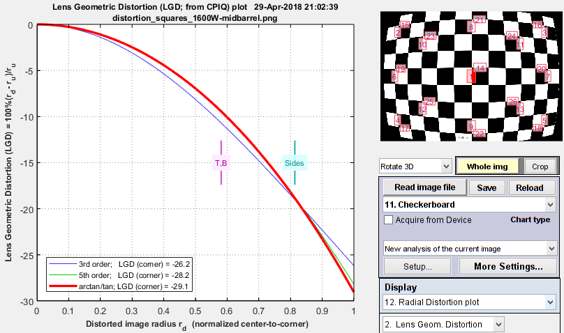 Checkerboard module Checkerboard module |
||
Notes: the third order calculations (Distortion and SFRplus) are less accurate than the fifth order and arctan/tan calculations (i.e., they cannot be as good a fit to the actual distortion.) The green line (SMIA TV Distortion) in the Dot Pattern figure cannot be compared with the other figures.
Links
Wikipedia Distortion (optics) page. A good read (not long). Claims that the division model is more accurate.
Edmund Optics Distortion application note