|
Aliasing |
|
Low frequency artifacts, sometimes quite disturbing, that appear when the image sensor receives significant signal energy above the Nyquist frequency. Color aliasing in Bayer sensors can be particularly troublesome. “Moire fringing” is a type of aliasing. See diagram in Nyquist frequency, below. Controlled by means of Anti-Aliasing (Optical Lowpass) Filters, which blur the image slightly (a classic tradeoff). | |||||||||||||||||||||||||||||||||||||||||||||||||||||||||||||||||||||||||||||
|
Aperture |
|
The circular opening at the center of a lens that admits light. Generally specified by the f-stop (f-number), which is the focal length divided by the aperture diameter. A large aperture corresponds to a small f-stop. This can confuse beginners. |
|||||||||||||||||||||||||||||||||||||||||||||||||||||||||||||||||||||||||||||
|
Bayer sensor |
|
The sensor pattern used in most digital cameras, where alternate rows of pixels are sensitive to RGRGRG and GBGBGB light. (R = Red; G = Green; B = Blue.) The four possible arrangements of R, G, and B are shown here. To be usable, the sensor output must be converted into a standard file format (for example, JPEG, TIFF, or PNG), where each pixel represents all three colors, by a RAW converter (in the camera or computer), which performs a “demosaicing” function. The quality of RAW converters varies: separate converter programs run in computers may provide finer results than the converters built into cameras. That is one of the reasons that RAW format is recommended when the highest image quality is required. Imatest Master can analyze Bayer raw files. In Foveon sensors (used in Sigma cameras), each pixel site is sensitive to all three colors. Foveon sensors are less susceptible to color aliasing than Bayer sensors; they can tolerate greater response above Nyquist with fewer ill effects. |
|||||||||||||||||||||||||||||||||||||||||||||||||||||||||||||||||||||||||||||
|
Chromatic aberration (CA) |
|
A lens characteristic that causes different colors to focus at different locations. There are two types: longitudinal, where different colors to focus on different planes, and lateral, where the lens focal length, and hence magnification, is different for different colors. Lateral CA is the cause of a highly visible effect known as color fringing. It is worst in extreme wide angle, telephoto, and zoom lenses. Imatest SFR measures lateral CA (color fringing). Measurements are strongly affected by demosaicing; accurate measurements for lenses must be done on raw files, which can be done starting with Imatest Master 2.7. See Chromatic aberration and Eliminating color fringing. |
|||||||||||||||||||||||||||||||||||||||||||||||||||||||||||||||||||||||||||||
|
Cycles, Line Pairs, Line Width |
|
A Cycle is the period a complete repetition of a signal. It is used for frequency measurement. A Cycle is equivalent to a Line Pair. Sometimes Line Widths are used for historical reasons. One Line Pair = 2 Line Widths. “Lines” should be avoided when describing spatial frequency because it is ambiguous. It usually means Line Widths, but sometimes it is used (carelessly) for line pairs. |
|||||||||||||||||||||||||||||||||||||||||||||||||||||||||||||||||||||||||||||
|
Demosaicing |
|
The process of converting RAW files, which are the unprocessed output of digital camera image sensors, into usable file formats (TIFF, JPEG, etc.) where each pixel has information for all three colors (Red, Green, and Blue). For Bayer sensors, each RAW pixel represents a single color in RGRGRG, GBGBGB, … sequence. Although demosaicing is the primary function of RAW converters, they perform additional functions, including adding a gamma curve and often an additional tonal response curve, reducing noise and sharpening the image. |
|||||||||||||||||||||||||||||||||||||||||||||||||||||||||||||||||||||||||||||
|
Density . . |
|
The amount of light reflected or transmitted by a given media, expressed on a logarithmic (base 10) scale. For reflective media (such as photographic or inkjet prints), density = –log10(reflected light/incident light). For transmissive media (such as film), density = –log10(transmitted light/incident light).The higher the density, the less light is transmitted or reflected. Perfect (100%) transmission or reflection corresponds to a density of 0; 10% corresponds to a density of 1; 1% corresponds to a density of 2, etc. Useful equations: 1 f-stop (1 EV) = 0.301 density units; 1 density unit = 3.32 f-stops (EV). When an object is photographed, Log10 Exposure = –density + k. (Constant k is generally ignored.) |
|||||||||||||||||||||||||||||||||||||||||||||||||||||||||||||||||||||||||||||
|
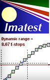
Dynamic range |
|
The range of exposure (usually measured in f-stops) over which a camera responds. Also called exposure range. Practical dynamic range is limited by noise, which tends to be worst in the darkest regions. Dynamic range can be specified as total range over which noise remains under a specified level— the lower the level, the higher the image quality. Dynamic range is measured by Stepchart, using transmission step charts. |
|||||||||||||||||||||||||||||||||||||||||||||||||||||||||||||||||||||||||||||
|
Exposure |
|
The definition depends on the context. 1. In Imatest results, “exposure” is the amount of light reaching a region of the sensor. Imatest plots often use Log Exposure (where Log is log10 in this context) because the human eye’s response is roughly logarithmic. For test chart images, Log exposure is proportional to −optical density. 2. In other contexts “exposure” may refer to the combination of exposure time and lens aperture, which can be expressed quantitatively in EV. |
|||||||||||||||||||||||||||||||||||||||||||||||||||||||||||||||||||||||||||||
|
Exposure value (EV) |
|
A measure of exposure (definition 2), where a change of one EV corresponds to doubling or halving the total light reaching the image plane. Often synonymous with f-stop (in the context of exposure change). By definition, 0 EV is a 1 second exposure at f/1.0. EV = log2(N2/t) where N = f-stop and t = exposure time. Note that EV is based on log2 while density is based on log10. (Here in Boulder, Colorado, residents prefer to use “enlightenment”, which is based on natural logarithms (loge, where e = 2.71828…). Boulderites strongly prefer products labeled “natural”, “organic”, or “green”, or prefixed “eco-“, “enviro-“, etc. 1 Enlightenment Unit (€) = 0.4343 Density units = 1.443 EV.) |
|||||||||||||||||||||||||||||||||||||||||||||||||||||||||||||||||||||||||||||
|
f-stop . |
|
A measure of the a lens’s aperture (the circular opening that admits light). A a change of “one f-stop” implies doubling or halving the exposure. This is the synonymous with a change of 1 EV (or zone from Ansel Adams’ zone system). F-stop = focal length / aperture diameter. The notation, “f/8,” implies (aperture diameter = ) focal length/8. The larger the f-stop number, the smaller the aperture. F-stops are typically labeled in the following sequence, where the admitted light decreases by half for each stop: 1, 1.4, 2, 2.8, 4, 5.6, 8, 11, 16, 22, 32, 45, 64, … Each f-stop is the previous f-stop multiplied by the square root of 2. |
|||||||||||||||||||||||||||||||||||||||||||||||||||||||||||||||||||||||||||||
|
Gamma |
|
Exponent that relates pixel levels in image files to the brightness of the monitor or print. Most familiar from displays, where luminance = pixel levelgamma. A camera (or film + scanner) encodes the image so that pixel level = brightness(camera gamma) (approximately). Several Imatest modules report camera gamma: Stepchart, Colorcheck, Multicharts, SFRplus and SFR (when chart contrast is known), and Star Chart. Gamma is equivalent to contrast. This can be observed in traditional film curves, which are displayed on logarithmic scales (typically, density (log10(absorbed light) vs. log10(exposure)). Gamma is the average slope of this curve (excluding the “toe” and “shoulder” regions near the ends of the curve), i.e., the contrast. See Kodak’s definition in Sensitometric and Image-Structure Data. For more detail, see the descriptions of gamma in Using Imatest SFR and Monitor calibration. For digital cameras, log pixel level is plotted as a function of log exposure (– chart density). Gamma is the average slope of this curve, excluding the brightest (often saturated) and darkest (not visually significant) patches. For example, for the Colorchecker, patches 2-5 of the bottom row (patches 20-23 of the entire chart; light to dark gray) are used. Confusion factor: Digital cameras output may not follow an exact gamma (exponential) curve: A tone reproduction curve (usually an “S” curve) may be superposed on the gamma curve to boost visual contrast without sacrificing dynamic range. Such curves boost contrast in middle tones while reducing it in highlights and shadows. Tone reproduction curves may also be adaptive: camera gamma may be increased for low contrast scenes and decreased for contrasty scenes. (Hewlett-Packard advertises this technology.) This can affect the accuracy of SFR measurements. But it’s not a bad idea for image making: it’s quite similar to the development adjustments (N-1, N, N+1, etc.) Ansel Adams used in his zone system. |
|||||||||||||||||||||||||||||||||||||||||||||||||||||||||||||||||||||||||||||
|
Image editor |
|
An image editor is a program for editing and printing images. The most famous is Adobe Photoshop, but Picture Window Pro is an excellent choice for photographers (though it doesn’t have all the graphic arts features of Photoshop). If you don’t have one, get Irafanview, which is more of an image viewer— a program for reading, writing, and viewing images. Irafnview can read and write images in almost any known format, and it also includes simple editing capabilities. Image editors contain more sophisticated functions, like masks, curves, and histograms. |
|||||||||||||||||||||||||||||||||||||||||||||||||||||||||||||||||||||||||||||
|
ISO speed |
|
The sensitivity of a camera to light. Sometimes called Exposure Index. The higher the ISO speed, the less exposure is required to capture an image. In digital cameras ISO speed is adjusted by amplifying the signal from the image sensor prior to digitizing it (A-D conversion). This increases noise along with the image signal. ISO speed was called ASA speed in the old days. See Kodak Application Note MTD/PS-0234: ISO Measurement and Wikipedia. |
|||||||||||||||||||||||||||||||||||||||||||||||||||||||||||||||||||||||||||||
|
Lens |
Lens (optical) distortion is an aberration that causes straight lines to curve near the edges of images. It can be troublesome for architectural photography and photogrammetry (measurements derived from images). See Distortion. |
||||||||||||||||||||||||||||||||||||||||||||||||||||||||||||||||||||||||||||||
|
MTF |
|
Modulation Transfer Function. Another name for Spatial Frequency Response (SFR). Indicates the contrast of a pattern at a given spatial frequency relative to very low spatial frequencies. See Sharpness and Understanding image sharpness and MTF curves. |
|||||||||||||||||||||||||||||||||||||||||||||||||||||||||||||||||||||||||||||
|
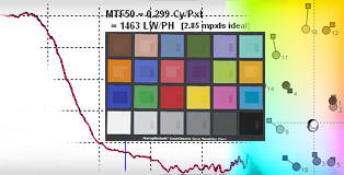
MTF50 |
|
The spatial frequency where image contrast is half (50%) that of low frequencies. MTF50 is an excellent measure of perceived image sharpness because detail is diminished but still visible, and because it is in the region where the response of most cameras is declining most rapidly. It is especially valuable for comparing the sharpness of different cameras. See Sharpness and Understanding image sharpness and MTF curves. |
|||||||||||||||||||||||||||||||||||||||||||||||||||||||||||||||||||||||||||||
|
MTF50P |
|
The spatial frequency where image contrast is half (50%) the peak value. MTF50P is the same as MTF50 in imaging systems with little to moderate sharpening, but is lower for systems with heavy sharpening, which have a peak in their MTF response. MTF50P is increased less than MTF in strongly oversharpened cameras; it may be a better measurement of perceived image sharpness than MTF50 in such cases. See Sharpness and Understanding image sharpness and MTF curves. |
|||||||||||||||||||||||||||||||||||||||||||||||||||||||||||||||||||||||||||||
|
Noise |
|
Random variations of image luminance arising from grain in film or electronic perturbations in digital sensors. Digital sensors suffer from a variety of noise mechanisms, for example, the number of photons reaching an individual pixel or resistive (Johnson) noise. Noise is a major factor that limits image quality. In digital sensors it tends to have the greatest impact in dark regions. It is worst with small pixels (under 3 microns). Noise is measured as an RMS value (root mean square; an indication of noise power, equivalent to standard deviation, sigma). Software noise reduction, used to reduce the visual impact of noise, is a form of lowpass filtering (smoothing) applied to portions of the image that to not contain contrasty features (edges, etc.). It can cause a loss of low contrast detail at high spatial frequencies. The Log F-Contrast module was designed to measure this loss. The visual impact of noise is also affected by the size of the image— the larger the image (the greater the magnification), the more important noise becomes. Since noise tends to be most visible at medium spatial (actually angular) frequencies where the eye’s Contrast Sensitivity Function is large, the noise spectrum has some importance (though it is difficult to interpret). To learn more, go to Noise in photographic images. |
|||||||||||||||||||||||||||||||||||||||||||||||||||||||||||||||||||||||||||||
|
Nyquist frequency |
|
The highest spatial frequency where a digital sensor can capture real information. Nyquist frequency fN = 1/(2 * pixel spacing) = 0.5 cycles/pixel. Any information above fN that reaches the sensor is aliased to lower frequencies, creating potentially disturbing Moire patterns. Aliasing can be particularly objectionable in Bayer sensors in digital cameras, where it appears as color bands. The ideal lens/sensor system would have MTF = 1 below Nyquist and MTF = 0 above it. Unfortunately this is not achievable in optical systems; the design of anti-aliasing (lowpass) filters always involves a tradeoff that compromises sharpness.
In this simplified example, sensor pixels are shown as alternating white and cyan zones in the middle row. By definition, the Nyquist frequency is 1 cycle in 2 pixels. The signal (top row; 3 cycles in 4 pixels) is 3/2 the Nyquist frequency, but the sensor response (bottom row) is half the Nyquist frequency (1 cycle in 4 pixels)— the wrong frequency. It is aliased. A large MTF response above fN can indicate potential problems with aliasing, but the visibility of the aliasing is much worse when it arises from the sensor (Moire patterns) than it is when it arises from sharpening (jagged edges; not as bad). It is not easy to tell from MTF curves exactly which of these effects dominates. The Nyquist sampling theorem and aliasing contains a complete exposition. |
|||||||||||||||||||||||||||||||||||||||||||||||||||||||||||||||||||||||||||||
|
Raw files Raw conversion |
|
RAW files are the unprocessed output of digital camera image sensors, discussed in detail here. For Bayer sensors, each RAW pixel represents a single color in RGRGRG, GBGBGB, … sequence. To be converted into usable, standard file formats (TIFF, JPEG, etc.), raw files must be run through a RAW converter (demosaicing program). RAW converters perform additional functions: they add the gamma curve and often an additional tonal response curve, and they reduce noise and sharpen the image. This can interfere with some of Imatest’s measurements. The best way to be sure an image file faithfully resembles the RAW file— that it has no sharpening or noise reduction— is to read a RAW file into Imatest, which uses Dave Coffin’s dcraw to convert it to a standard format (TIFF or PPM). Imatest documentation sometimes distinguishes between camera RAW files— camera manufacturer’s proprietary formats, and Bayer RAW files— undemosaiced files that contain the same data as camera raw files, but are in standard easily-readable formats such as TIFF or PGM. Dcraw can convert camera RAW files into Bayer RAW files. Starting with version 2.7, several Imatest Master modules can measure camera RAW files directly. |
|||||||||||||||||||||||||||||||||||||||||||||||||||||||||||||||||||||||||||||
|
Resolution |
|
The first thing to remember about resolution is that it has no unique definition. It can be defined in many ways, some of which can be quite misleading. (It is almost as abused as the word “holistic.”) In a generic sense, resolution refers to any measurement of an imaging system’s ability to resolve fine detail. For traditional film cameras, it usually refers to vanishing resolution— the highest spatial frequency where the pattern on a bar chart (usually the USAF 1951 chart) was visible. Since this tells you where detail isn’t, it’s not a very good indicator of perceived sharpness. The pixel per inch (PPI or DPI) rating of a scanner is often called its “resolution.” This can be highly misleading. For example, some inexpensive flatbed scanners can’t come close to resolving the detail of decent film scanners with the same PPI rating; their lenses aren’t up to the job. I prefer MTF50 (the spatial frequency where contrast falls to half its low frequency value) as a measure of resolution. For more on resolution, see Pixels, Images, and Files and Lens testing (the old-fashioned way). |
|||||||||||||||||||||||||||||||||||||||||||||||||||||||||||||||||||||||||||||
|
SFR |
|
Spatial Frequency Response. The response of a system to a pattern at a given spatial frequency, i.e., the contrast. SFR is measured relative to contrast at very low spatial frequencies. It is expressed as a fraction or percentage. Synonymous with MTF. See Sharpness and Understanding image sharpness and MTF curves. |
|||||||||||||||||||||||||||||||||||||||||||||||||||||||||||||||||||||||||||||
|
Sharpening |
|
Signal processing applied to digital images to improve perceived image sharpness. It can be applied in the camera or in post-processing (image editing). Virtually all digital images benefit from some degree of sharpening, but images can be oversharpened, resulting in highly visible “halos” (overshoots) near edges. MTF can have values larger than 1 as a result of sharpening. See Sharpening. |
|||||||||||||||||||||||||||||||||||||||||||||||||||||||||||||||||||||||||||||
|
Standardized sharpening |
|
A now-deprecated algorithm that attempted to enable cameras with different amounts of sharpening to be compared fairly. With standardized sharpening, all cameras have a similar amount of overshoot (around 5%) near edges. Without it, built-in sharpening strongly affects test results, giving oversharpened cameras an unfair advantage. Results with standardized sharpening should not be used for comparing different lenses on the same camera. See Standardized sharpening. |
|||||||||||||||||||||||||||||||||||||||||||||||||||||||||||||||||||||||||||||
|
Tone reproduction curve (TRC) |
|
A curve that describes a camera’s response to light. Usually displayed as Density or Log pixel level vs. Log exposure. Often refers to an “S”-shaped or “shouldered” curve applied on top of the gamma curve during Raw conversion. (The “shoulder” is rounding of the upper part of the curve.) The purpose of such a TRC is to (1) increase visible (midtone) contrast while maintaining detail in the highlights and sometimes shadows, and (2) to reduce the likelihood of highlight saturation in contrasty scenes. Known as the H&D Curve in the good ol’ days of film. |
|||||||||||||||||||||||||||||||||||||||||||||||||||||||||||||||||||||||||||||
|
Uniformity |
|
Uniformity measures lens vignetting (dropoff in illumination at the edges of the image) and other image nonuniformities. For example it can measure evenness of flash illumination (using light bounced off a white wall) or the uniformity of flatbed scanners. In Imatest, Uniformity can also analyze color shading (nonuniformity), hot and dead pixels, display a pixel level histogram, a grid (sector) plot, and a detailed image of fine nonuniformities (i.e., sensor noise). These features are described in Using Uniformity, Part 2. |
|||||||||||||||||||||||||||||||||||||||||||||||||||||||||||||||||||||||||||||
|
Uniformity-Interactive |
|
Uniformity-Interactive measures image nonuniformity, which can be caused by the lens, the sensor, and the lighting— the same parameters measured by Uniformity— in an interactive interface that can be updated in near-realtime. See Using Uniformity-Interactive. |
Links to other glossaries
SPIE Optipedia An outstanding resource for optics.
Hewlett Packard’s Digital Glossary
Canon EF Lens 101 Glossary An excellent resource: more detail than you’d expect.
Solid State Image Sensors: Terminology (a Kodak Application Note) Relatively technical, but valuable.
 |
 |
 |
