More settings window – Secondary Readout – Settings area – Auto mode window
Warnings – Clipping – Summary
Running Checkerboard (Interactive and Auto mode settings)
Imatest Checkerboard performs highly automated measurements of sharpness (expressed as Spatial Frequency Response (SFR), also known as Modulation Transfer Function (MTF)), Lateral Chromatic Aberration , and optical distortion from tilted checkerboard images.The primary advantage of Checkerboard is that the field of view, i.e., the framing, does not need to be tied to the chart size (as it does with SFRplus and eSFR ISO). You can zoom in as much as you want as long as there are sufficient edges to analyze, and you can zoom out as far as you want (though the outer parts of the image might not be analyzed if you zoom out too far).
This document shows how to run Checkerboard in Rescharts and how to save settings for automated runs. Part 1 introduced Checkerboard and explained how to obtain and photograph the chart. Part 3 illustrates the results.
 Open Imatest by double-clicking the Imatest icon
 ![]() on
on
- the Desktop,
- the Windows Start menu,
- the Imatest folder (typically C:Program files\Imatest\vm.n\Edition (where m.n is the version, e.g., 4.2, and Edition can be Master, Image Sensor, etc.) in English language installations).
Checkerboard operates in two modes: interactive/setup and automatic.
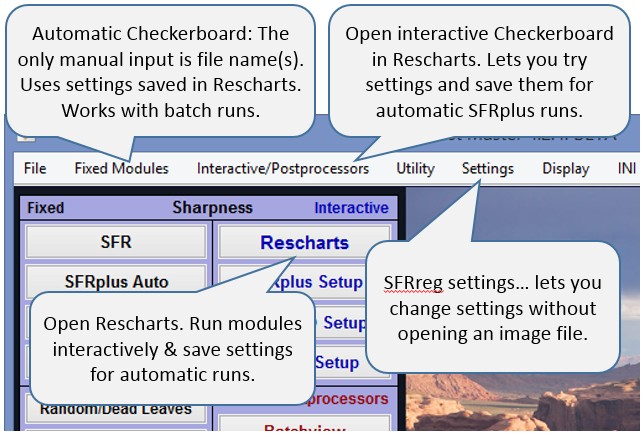
To initiate an interactive Checkerboard run (in Rescharts), press then 11. Checkerboard or press the Interactive/Postprocessors dropdown menu then Checkerboard setup. This opens a dialog box for reading an Checkerboard image file; pressing is more general; it lets you open any Rescharts module. Either of these buttons allows you to analyze a checkerboard image, examine detailed results interactively, and save settings for the highly automated Checkerboard auto runs (or the even more automated Imatest IT EXE or DLL versions). Checkerboard should be run at least once interactively prior to the first Checkerboard auto run. Checkerboard settings can also be updated by pressing Settings, Checkerboard Auto settings from the Imatest main window.
Rescharts Checkerboard
Selecting file(s)
 The portion of the Rescharts window used for opening files is shown on the right. You can open a file by clicking on if the correct chart type is displayed, or by selecting a Chart type. One or more files may be selected, as shown below. If you select multiple files, they can be combined (averaged), and you’ll be given the option of saving the combined file.
If the folder contains meaningless camera-generated file names such as IMG_3734.jpg, IMG_3735.jpg, etc., you can change them to meaningful names that include focal length, aperture, etc., with the View/Rename Files utility, which takes advantage of EXIF data stored in each file.
The folder saved from the previous run appears in the Look in: box on the top. You are free to change it. The file name from the previous run is displayed at the bottom. You can open a single file by simply double-clicking on it. You can select multiple files for combined runs (for interactive or Checkerboard auto runs) or for batch runs (for Checkerboard auto-only) by the usual Windows techniques: control-click to add a file; shift-click to select a block of files. Then click . Three image files are highlighted. Large files can take several seconds to load.
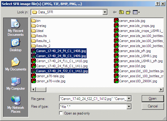
File selection
| Multiple file selection Several files can be selected in Imatest Master using standard Windows techniques (shift-click or control-click). For Colorcheck interactive (Rescharts) runs, files can be combined to reduce noise or (in some instances) observe the effects of camera shake or image stabilization. For Colorcheck Auto runs, you can run large batches of images. The multi-image dialog box gives you the option of saving the combined file, which will have the same name as the first selected file with _comb_n appended, where n is the number of files combined. |
| RAW files Imatest can analyze raw files from cameras (using dcraw) or from development systems (using Generalized Read Raw). The files can be demosaiced or converted to Bayer raw: standard files (TIFF, etc.) that contain undemosaiced data. Undemosaiced files are not very useful for measuring MTF because the pixel spacing in each of the four image planes is twice that of the image as a whole; hence MTF is lower than for demosaiced files. But Chromatic aberration can be severely distorted by demosaicing, and is best measured in Bayer RAW files (and corrected during RAW conversion). Details of RAW files can be found here |
Checkerboard setup window
When the file (or files) have been opened, the Checkerboard setup window, shown below, appears. This window allows you to select groups of regions (ROIs; shown as violet rectangles) for analysis. It also lets you select the size of the regions, whether to analyze vertical or horizontal edges, and much more. Pressing on the left opens the Checkerboard More settings, which allows you to select additional settings that affect the calculations and display. Pressing lets you select the output figures and files (for Checkerboard auto mode runs). The light yellow-orange rectangles are for calculating the Color/lightness uniformity profiles.
 Checkerboard setup window
| Checkerboard setup window |
|
| Settings area | |
| Gamma | Assumed Gamma (contrast) of the chart. Has a small effect on the MTF results. Default is 0.5. Overwritten if the Use for MTF checkbox (below Chart contrast) is checked. Gamma is described in more detail below. |
| Channel | Select channel to analyze: R, G, B, Y, R-only, G-only, B-only, Y-only. (Y is Luminance channel). Use one channel only to speed up calculations or where other channels are dark or may not contain valid data. Selecting one channel-only can significantly speed up calculations. |
| Chart contrast (for gamma calc.) |
Chart contrast– for the contrasty squares (i.e., most of them). Used to estimate gamma from the image. |
| Use for MTF | (Checkbox, normally unchecked) When checked, the gamma derived from the chart is used for the MTF calculation. This may result in a small improvement in accuracy. |
| Open the Checkerboard More settings window, shown below. | |
| Open the Checkerboard Auto mode settings window, shown below, for controlling . | |
| ROI Selection & analysis area Selects which regions (ROIs) to analyze. Corners are located automatically. Choices below. These are particularly important settings. |
|
| Target Detection Settings (lower-left of ROI selection area) |
The routine for checkerboard corner point detection can be selected from the Checkerboard Target Detection window. Tuning options are available for images for which default detection fails to cover the required target area. |
| Region selection (Selects which regions to locate. Actual ROIs are located automatically) |
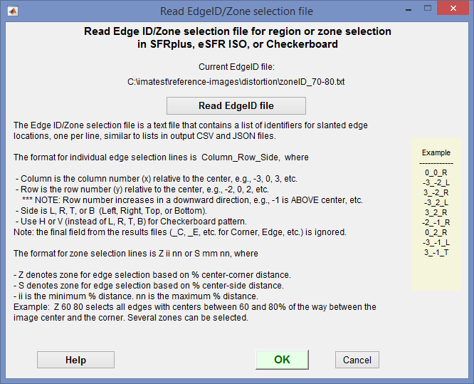
Select the regions (ROIs) to analyze. Choices below. The number of regions is in parentheses. This is a particularly important setting. We encourage users to become familiar with the settings below. At least 13 regions are required for 3D plots. 1. Center (1) 2. Read Edge ID/Zone selection file. An Edge ID/Zone selection file contains a list of identifiers for slanted edge ROI locations or selection zones, one per line, similar to lists in CSV and JSON output files. There are two types of data line: for individual ROIs and for ROI selection zones. It allows you to freely select edges or zones.
Click Read EdgeID file to read the file. Then click OK. Individual edge ROI selection lines: the format is Column_Row_Side, where
Example: -2_1_V selects a vertical edge of the square two columns left of center and one row below center (defined as the intersection of the three dots, shown above). Zone selection lines (Imatest 5.0+): the format is Z ii nn or S ii nn, where
Example: Z 60 80 selects all edges with centers between 60 and 80% of the way between the image center and the corner. Several zones can be selected. 3. Use most recent EdgeID file. 4. Center & corners (5) 5. Center, corners, part-way (9) (Part-way on diagonal between center & corners) 6. Center, L, R, T, B (5) 7. Center, corners, L, R, T, B (9) 8. Center, corners, part-way, L, R, T, B (13) This is the smallest selection that can be used with 3D displays. This setting is often a good compromise between speed and detail. 9. 5 rows, 5 columns (for odd number of rows ≥ 5) (25) (edges on a 5×5 grid). Detailed results, well-suited for 3D displays. 10. All sqares. Very detailed. May run somewhat slow (depending on number of rows and columns).
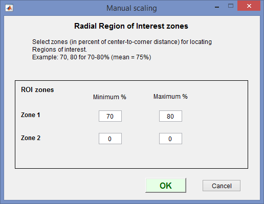
12. Alt squares 1 (start at 1,2) 13. Alt squares 1 (start at 3,1) 14. Alt squares 1 (start at 2,2) 15,16 (Currently not used) 17. Selected ROI zones (% from ctr). Lets you select edges (you can specify Horizontal or Vertical elsewhere) within one or two radial zones. The default is shown in the figure on the right: one zone where edges whose edge centers are located at 70-80% of the center-to-corner distance. 18. NO regions: fast geometry calculation (for distortion calculation-only) |
| Vertical, Horizontal edges (or both) |
Chooses between Vertical and Horizontal edges (or both). Usually Vertical, but Horizontal is useful on occasion. Use both for Lens-style MTF plots. For 3D plots it’s best to plot Horizontal or Vertical-only. |
| Speedup (checkbox) | Speed up the run by eliminating some calculations that many users don’t require, including SQF/Acutance, noise statistics and histograms. |
| ROI size | Slider that determines the size of the ROI. Use the largest value that keeps a save distance from edges of squares and top and bottom bars. May need to be reduced where distortion is severe. |
| Allows borders to be cropped to remove interfering patterns that might otherwise be included in the image. This button is tinted pink whenever the image is cropped. | |
| ROI width (below ROI size slider) |
Width of ROI selection. Normal width for the standard rectangular ROI. Choose Wider or Widest for very fuzzy edges, for enhanced noise analysis, or for more extended low frequency response. |
| Other controls | |
| Title | Title. Defaults to file name. You can add a description. |
| Open this web page in a web browser. | |
| Display … image | Selects image for Setup window display: Original (RGB) image, R, G, or B channel, lightened, color-boosted, etc. |
| Save settings (for use in auto Checkerboard), but do not continue with run. | |
| Save settings and continue with run: Calculate results for all selected region. You will be able to view results interactively. | |
| Cancel run; do not save settings | |
After you’ve finished making settings, click to save settings and continue with the run. You can Click to save the settings without continuing.
More settings window
The Checkerboard More settings window, shown below, opens when
- is pressed in the Checkerboard setup or Rescharts windows.
- Settings, Checkerboard settings is pressed in the Imatest main window, then is pressed in the Checkerboard setup window.
The settings are read from the imatest-v2.ini file, and saved when is pressed. Settings are similar to settings in the SFR input dialog box and also the SFRplus and eSFR ISO More settings windows with several settings removed.
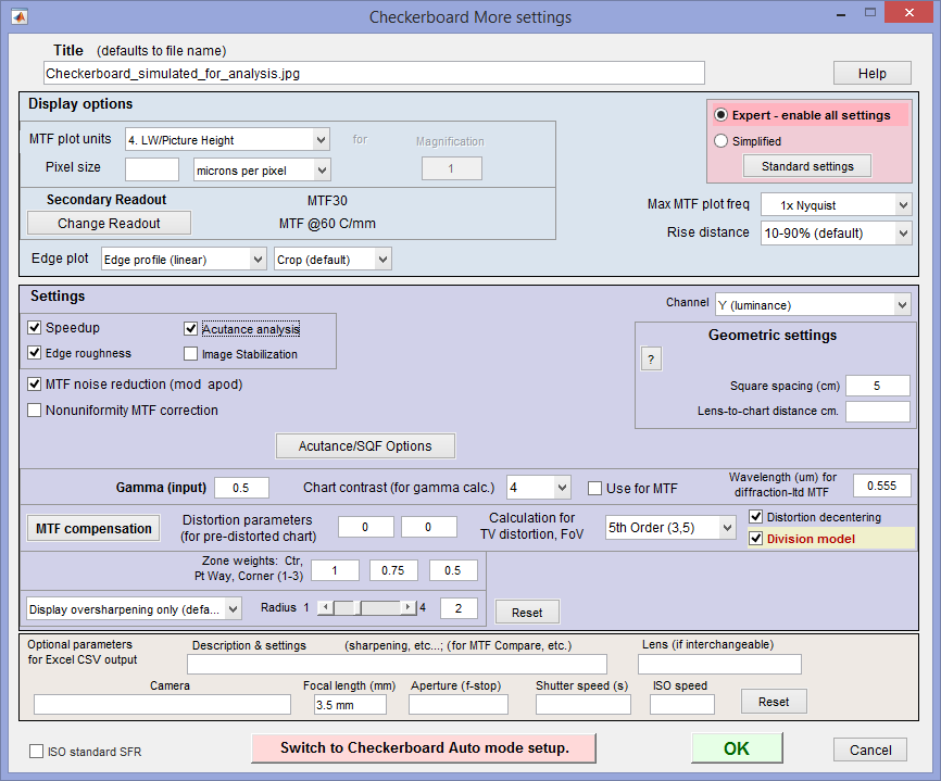 Checkerboard More settings window
| You can select either Expert or Simplified mode for the settings window. In Simplified mode many settings are grayed out so they can’t be set. If you press , commonly used settings (recommended for beginners) are selected. |
This window is divided into sections: Title and on top, then Display options, Settings, Optional parameters, and finally, or at the bottom.
Title defaults to the input file name. You may leave it unchanged, replace it, or add descriptive information for the camera, lens, converter settings, etc.— as you please.
opens a browser window containing a web page describing the module. The browser window sometimes opens behind other windows; you may need to check if it doesn’t pop right up.
| Display options (below Plot) contains settings that affect the display (units, appearance, etc.).
MTF plot units selects the spatial frequency scale for MTF plots for for the summary plot. Cycles/pixel (C/P), Cycles/mm (lp/mm), Cycles/inch (lp/in), Line Widths per Picture Height (LW/PH), Line Pairs per Picture Height (LP/PH), cycles/angle, and cycles/object distance are some of the choices. See the full list on the Sharpness page. (Note that one cycle is the same as one line pair or two line widths.) If you select Cycles per inch or Cycles/mm, you must enter a number for the pixel size— either in pixels per inch, pixels per mm, or microns per pixel. For more detail on pixel size, see the box below. note: for using picture height (LW/PH) or (LP/PH) units with cropped images enter the original picture height into the more settings dimensions input.
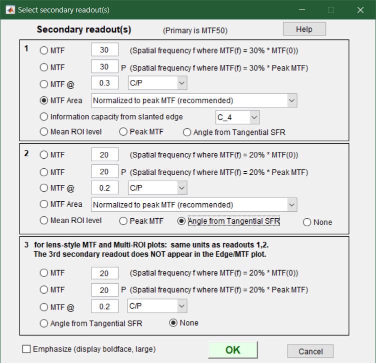
Maximum MTF plot frequency selects the maximum display frequency for MTF plots. The default is 2x Nyquist (1 cycle/pixel). This works well for high quality digital cameras, but not for imaging systems where the edge is spread over several pixels. In such cases, a lower maximum frequency produces a more readable plot. 1x Nyquist (0.5 cycle/pixel), 0.5x Nyquist (0.25 cycle/pixel), and 0.2x Nyquist (0.1 cycle/pixel), and others are available. Secondary readout controls the secondary readout display in MTF plots. The primary readout is MTF50 (the half-contrast spatial frequency). Two secondary readouts are available with several options. The first defaults to MTF30 (the spatial frequency where MTF is 30%). The third is used only for Lens-style MTF plots. Clicking Change opens the window shown on the right. Secondary readout settings are saved between runs. Choices:
|
Edge plot selects the contents of the upper (edge) plot. The edge can be cropped
(default) or the entire edge can be displayed. Three displays are available.
- Edge profile (linear) is the edge profile with gamma-encoding removed. The values in this plot are proportional to light intensity. This is the default display.
- Line spread function (LSF) is the derivative of the linear edge profile. MTF is the fast fourier transform (FFT) of the LSF.
- Edge pixel profile is proportional to the edge profile in pixels, which includes the effects of gamma encoding.
- Edge linear, unnormalized is similar to Edge profile (1.), but not normalized. Useful in diagnosing situations where one channel may be saturating (and affecting MTF measurements).
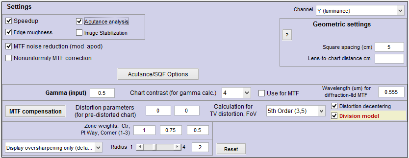
| Settings affect the results as well as the display.
Speedup Speed up calculatons by eliminating some calculations that many users don’t require, including noise statistics and histograms. Checking Speedup can significantly speed up calculations. Edge roughness Calculate edge roughness (for inclusing in CSV output). Slows calculations slightly. Required if Edge roughness plot is to be displayed. MTF noise reduction (mod apod) Reduce noise using the modified apodization technique. Improves MTF accuracy, especially with noisy images, but not an ISO standard calculation. Generally recommended. Channel specifies the primary channel to display (all channels are analyzed). It’s normally left at it’s default value of Y for the luminance channel, Square spacing in cm is used to calculate the Field of View (FoV) when Pixel spacing (pitch) has been entered. It is optional (not normally entered). For pre-distorted charts, use the square spacing closest to the center. FoV is displayed in Image & Geometry and reported in the CSV and JSON output files if calculated. Lens-to-chart distance in cm is used to calculate the actual lens focal length when Pixel spacing (pitch) and bar-to-bar chart height have been entered. It is optional. The distance from the lens to target is most conveniently measured with a laser measuring device. Focal length is displayed in Image & Geometry and reported in the CSV output file if calculated. Gamma (the average slope of log pixel levels as a function of log exposure for light through dark gray tones) is used to linearize the input data, i.e., to remove the gamma encoding applied by the camera or RAW converter. It defaults to 0.5 = 1/2, which is typical of digital cameras, but may be affected by camera or RAW converter settings. Small errors in gamma have little effect on MTF measurements (a 10% error in gamma results in a 2.5% error in MTF50 for a normal contrast target). Gamma should be set to 0.45 or 0.5 when dcraw is used to convert RAW images into sRGB or a gamma=2.2 (Adobe RGB) color space. It is typically around 1 for raw images that haven’t had a gamma curve applied. If gamma is set to less than 0.3 or greater than 0.8, the background will be changed to pink to indicate an unusual (possibly erroneous) selection. If the chart contrast is known and is ≤10:1 (medium or low contrast), you can enter the chart contrast in the Chart contrast (for gamma calc.) box, then check the Use for MTF checkbox. Gamma will be calculated from the chart and displayed in the Edge/MTF plot. If chart contrast is not known you should measure gamma from an image of a grayscale stepchart (a huge variety of grayscale charts is available) by running Colorcheck, Stepchart , Color/Tone Interactive (interactive), or Color/Tone Auto. A nominal value of gamma should be entered, even if the value of gamma derived from the chart (described above) is used to calculate MTF. |
| Gamma | |
| Gamma is the exponent of the equation that relates image file pixel level to luminance. For a monitor or print, Output luminance = (pixel level)gamma_display When the raw output of the image sensor, which is linear, is converted to image file pixels for a standard color space, the approximate inverse of the above operation is applied. pixel level = (RAW pixel level)gamma_camera ~= exposuregamma_camera The total system gamma is gamma_display * gamma_camera. Standard values of display gamma are 1.8 for older color spaces used in the Macintosh and 2.2 for color spaces used in Windows, such as sRGB (the default) and Adobe RGB (1998). In practice, gamma is equivalent to contrast. More on gamma can be found in SFR Instructions, part 2. |
|
Wavelength (um) for diffraction-limited MTF plot. If a number is entered (0.555 um is the default for visible light systems) and pixel spacing is also entered, the diffraction-limited MTF is displayed on the MTF plot and the diffraction-limited edge or Line Spread Function (cross-section of Airy disk) is shown on the edge plot as a faint dashed line MTF compensation (Imatest 5.1+) allows you to compensate for the measured chart MTF. This can double the megapixel suitability of a chart. Also allows you to remove a simple model of sensor MTF to get closer to lens MTF. Details in MTF compensation. Distortion Parameters (for pre-distorted chart) have not yet been implemented in Checkerboard.
Zone weights Weights of the center, part-way, and corner zones. Used for calculating weighted means of key results, displayed in the Multi-ROI and 3D plots. The defaults of 1 (center), 0.75 (part-war), and 0.5 (corners) are for typical pictorial photography; corners should probably be given more weight for technical photography. Standardized sharpening was intended to facilitate comparison of cameras with different degrees of sharpening, but is no longer recommended. If Standardized sharpening is ON, standardized sharpening results are displayed as thick red curves and readouts in the edge and MTF plots. If OFF (preferred), results for individual R, G, and B channels are displayed with more prominence and edge noise is displayed. Display oversharpening-only (described here) is recommended. See SFR instructions for more details. restores the settings in Checkerboard More Settings to their default values. |
| Additional parameters (all optional) for Excel .CSV output contains a detailed description of the camera, lens, and test conditions. EXIF data is entered, if available, but can be overridden by manual settings. Description & settings is particularly useful for annotating the test system (it is displayed in MTF Compare).These settings are optional but can be useful when several tests are run for different lenses, focal lengths, apertures, or other settings. The settings are displayed next to the MTF plots. If EXIF data is available (currently, only in JPEG files) it overrides any saved settings. The Reset button clears all entries. |
ISO standard SFR If this checkbox is checked, SFR calculations are performed according to the ISO 12233 standard, and the y-axis is labeled SFR (MTF) (ISO standard). This method is slightly less accurate than the normal Imatest calculation, which incorporates a number of refinements, including a better edge detection algorithm and a second-order polynomial fit to the average edge for a more accurate estimate of SFR in the presence of lens distortion. This box is normally left unchecked; it should only be used for comparing normal Imatest calculations to the ISO standard. The difference is typically very small.
When entries are complete, click to return control to the Checkerboard setup window or to save settings and return to the Imatest main window. When all entries are complete, click either , , or . saves the settings for use in automated Checkerboard runs, which can be initiated by clicking Fixed Modules (dropdown menu), Checkerboard Auto. (A button may be added in the future.) saves the settings then calculates results for interactive viewing. A sequence of Calculating… boxes appear to let you know how calculations are proceeding. When calculations are complete, results are displayed interactively in the Rescharts window.
Auto mode settings window
Auto mode settings affect plots and output files for Checkerboard Auto runs as well as Imatest IT/EXE and DLL. It does not directly affect interactive (Rescharts) runs. The Checkerboard Auto mode settings window, shown below, opens when
- Auto mode settings is pressed in the Checkerboard setup window.
- More settings is pressed in the Rescharts window, then Switch to Checkerboard Auto mode setup is pressed in the More settings window.
- Settings, Checkerboard Auto settings is pressed in the Imatest main window.
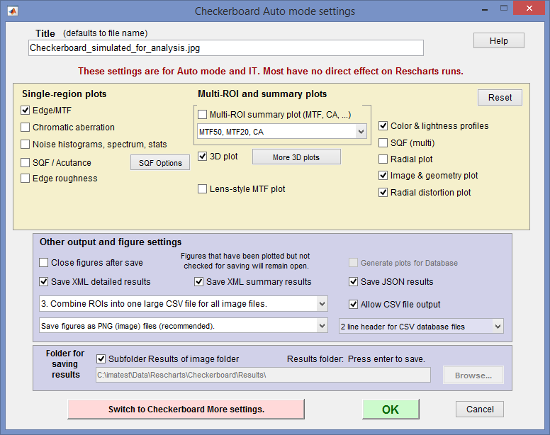 Checkerboard auto mode settings
The upper box allows you to select single and multi region figures to be plotted and saved in Checkerboard auto output. For the most part they are self-explanatory. Note that all plotted figures are saved.
Saved figures, CSV, XML, and JSON files are given names that consist of a root file name (which defaults to the image file name) with a suffix added. Examples:
Canon_17-40_24_f8_C1_1409_YR7_cpp.png
Canon_17-40_24_f8_C1_1409_YR7_MTF.csv
When 3D plot is checked, Checkerboard Auto plots the last 3D plot displayed in Rescharts unless the button has been pressed and one or more plots has been selected. More 3D plots will be displayed in pink in this case. This allows several 3D plots to be displayed and saved by Checkerboard auto.
Close figures after save should be checked if a large number of figures are to be displayed. It prevents a buildup of figures, which can slow processing.
Figures can be saved as PNG or FIG files. PNG files (a losslessly-compressed image file format) are the default— they require the least storage. Matlab FIG files allow the data to be manipulated– Figures can be resized, zoomed, or rotated (3D figures-only), but FIG files should rarely be used because they can be huge. PNG files are preferred if no additional manipulation is required.
A CSV summary file is saved for all runs. An XML file is saved if Save XML results is checked.
You can select either Save CSV files for individual ROIs or Save summary CSV file only (the summary file is always saved).
Save folder determines where results are stored. It can be set either to subfolder Results of the image folder or to a folder of your choice. Subfolder Results is recommended because it is easy to find if the image folder is known.
Limiting Distortion Analysis to The Image Circle
Distortion measurements may be limited to an image circle. Enabling limiting distortion analysis to an image circle is only available for distortion measurements (other measurements will be disabled). When enabled, the distance normalization factor is the image circle radius. When disabled, the distance normalization factor is the center-corner distance.
This setting is only available from the new Imatest front end. Go to Settings → Sharpness → Checkerboard → Image Circle.
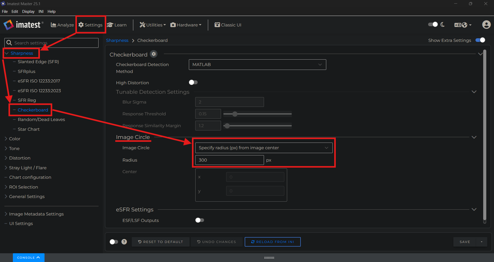
Location of Image Circle Settings
The options are
| Option | Description | Additional Inputs |
|---|---|---|
| None | Do not limit to the image circle | |
| Specify radius (px) from image center | Specify an image circle radius about the numeric center of the image | Radius [px] |
|
Specify radius and center
|
Specify an image circle radius about a user-provided point. The point is in IEEE Std 2020:2024 Type IV image coordinates (one-indexed from upper left). | Radius [px], Center |
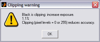
Warnings
| A Clipping warning is issued if more than 0.5% of the pixels are clipped (saturated), i.e., if dark pixels reach level 0 or light pixels reach the maximum level (255 for bit depth = 8). This warning is emphasized if over 5% of the pixels are clipped. Clipping reduces the accuracy of SFR results. It makes measured sharpness better than reality. |
 |
|
| The percentage of clipped pixels is not a reliable index of the severity of clipping or of MTF measurement error. For example, it is possible to just barely clip a large portion of the image with little loss of accuracy. The plot on the right illustrates strong clipping, indicated by the sharp corner near the “shoulder” on the black line. The MTF measurement is better than reality. The absence of a sharp corner indicates that there is little MTF error.Clipping can usually be avoided with a correct exposure— neither too dark nor light— and by avoiding high contrast targets (like the old ISO-12233 chart). The maximum recommended edge contrast is 10:1; 4:1 contrast (recommended in the upcoming revision to the ISO-12233 standard) is even better. Low-contrast targets are more reliable overall: in addition to better exposure latitude (reduced risk of clipping), they tend to have less sharpening in cameras with variable signal processing, and MTF results are less sensitive to errors in estimating gamma. |
Clipping warnings |

Checkerboard summary
- Checkerboard analyzes images of checkerboard patterns. Framing is not critical as long as at least four corners can be detected (more are usually recommended). There should be few or no interfering patterns (resembling checkerboard corners) outside the chart.
- Lighting should be even and glare-free. Lighting and alignment recommendations are given in The Imatest test lab.
- The first time Checkerboard is run, it should be run through Rescharts. This allows
- parameters to be adjusted and saved for later use in the automatic version of Checkerboard, which is opened by pressing Fixed modules (dropdown menu), Checkerboard Auto in the Imatest main window.
- results (listed above) to be examined interactively in the Rescharts window.
Next: Using Checkerboard Part 3: Results
Pixel sizePixel size is closely related to image quality. For very small pixels, noise, dynamic range and low light performance suffer. Pixel size is rarely given in camera spec sheets: it usually takes some math to find it. If the sensor type and the number of horizontal and vertical pixels (H and V) are available, you can find pixel size from the table on the right and the following equations. pixel size in mm = (diagonal in mm) / sqrt( H2 + V2 ) Pixel size in microns (microns per pixel) can be entered directly into the SFR settings box. Example, the cute little 5 megapixel Panasonic Lumix DMC-TZ1 has a 1/2.5 inch sensor and a maximum resolution of 2560x1980 pixels. Guessing that the diagonal is 7 mm, pixel size is 2.1875 (rounded, 2.2) microns.You can find detailed sensor specifications in pages from Sony, Panasonic, and Kodak. |
|
