|
Related pages Dynamic Range a comprehensive introduction: strongly affected by flare light. Veiling glare (lens flare) describes several measurement techniques, including the new Contrast Resolution method. Making Dynamic Range Measurements Robust Against Flare Light |
Introduction – Background – The Contrast Resolution chart – Photographing & analyzing –
Tonal response and SNR – Visualization – Visual analysis – Contrast Resolution Dynamic Range –
Tone mapped results – Flare Mask & two-image measurement – Summary – Verification – References
Introduction
 This page describes the Imatest Contrast Resolution chart and analysis (supported by Imatest 5.0+), which is designed to measure the visibility of low contrast objects in larger fields over a wide range of brightness. These measurements are expressed as the Contrast Resolution Signal-to-Noise Ratio (SNRCR) and Dynamic Range (DRCR). They are of particular interest to the automotive and security industries. This method of dynamic range measurement was inspired by a talk by Ulrich Seger of Robert Bosch at AutoSens 2016. It is compared with other methods in the Dynamic Range page.
Compared to standard Dynamic Range measurements, Contrast Resolution results are insensitive to errors caused by uncompensated black level offsets, flare light, and tone mapping, and the visibility of low contrast features can be clearly visualized over a wide range of tones.
We are introducing the chart to relevant standards committees, especially the IEEE P2020 Automotive System Image Quality group. We described the chart at AutoSens 2017 and Electronic Imaging 2018. The paper is available for download here.
Background
Camera Dynamic Range (the range of tones a camera responds to with good contrast and Signal-to-Noise Ratio (SNR)) is a function of the sensor and lens (and to some extent, the signal processing). Modern High Dynamic Range (HDR) sensors boast impressive dynamic ranges of 120 dB (a 1,000,000:1 brightness ratio) or more, but when a lens is placed in front of a sensor, flare light (stray light reflected between lens elements and off the lens barrel) limits the system (camera) dynamic range to 100 dB or less. (If you think your system can do better and you have data to back it up, please write us at [email protected]. We’ll be delighted to engage with you.)
Flare light is frequently measured from small pure black fields (“black holes” or light traps in reflective charts) in white fields, which usually extend beyond the image boundaries. Imatest’s older measurement of veiling glare (which indicates susceptibility to flare) is from the Stepchart module; Imatest 5.0+ has added the ISO 18844 flare measurement to the Uniformity module. After the image has been linearized and black level offsets (if any) have been removed,
Veiling glare = dark level/white level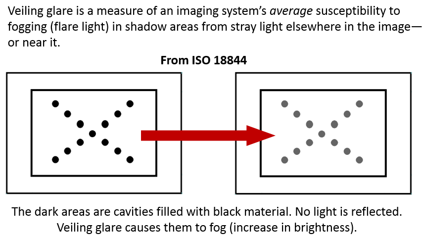 The problem with ISO 18844 flare/veiling glare measurements is (1) they cannot be directly related to the visibility of low contrast features in dark areas of the image, (2) they tend to exaggerate the damage caused by flare (i.e., a camera with a 120 dB HDR sensor may show only 50 dB of apparent dynamic range with this measurement), and (3) they are based on an inadequate model of the origin of flare, which is primarily caused by secondary reflections in multi-element lenses. The fogging from there reflections, which are not focused when they reach the image sensor, falls off with distance from bright features.
Standard dynamic range measurements are typically made with transmissive grayscale step charts that have a density range greater than the dynamic range of the camera. While they show overall density response, they don’t give good results for tone-mapped images, which widely used for HDR images processed for human viewing. Tone mapping selectively adjusts the tones in the image, lightening dark areas to make them visible in monitors with limited dynamic range. The tone-mapped image on the right below was obtained by applying the Matlab tone map function with 8 tiles (the default) in the Imatest Image Processing module to the image on the left.
| Crop of an image of the Imatest High Dynamic Range test chart, showing effects of tone mapping | |
 Original Original |
 Tone mapped Tone mapped |
 Density response— Original Density response— Original |
 Density response— Tone mapped Density response— Tone mapped |
Plots of log pixel level vs. exposure (-chart density) for tone-mapped images show low and inconsistent differences between patches, which is not at all indicative of the actual visibility of low contrast features within the patches. Tone mapping generally spoils tonal response measurements from conventional grayscale charts.
Standard Dynamic Range measurements are also subject to errors caused by flare light, which increases the signal level in SNR calculations— but signals from flare light are spurious since flare light arises from image features (generally brightly lit areas) outside the measurement area.
The Contrast Resolution chart was developed to overcome shortcomings of both traditional flare/veiling glare and dynamic range measurements.
The Contrast Resolution chart
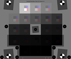
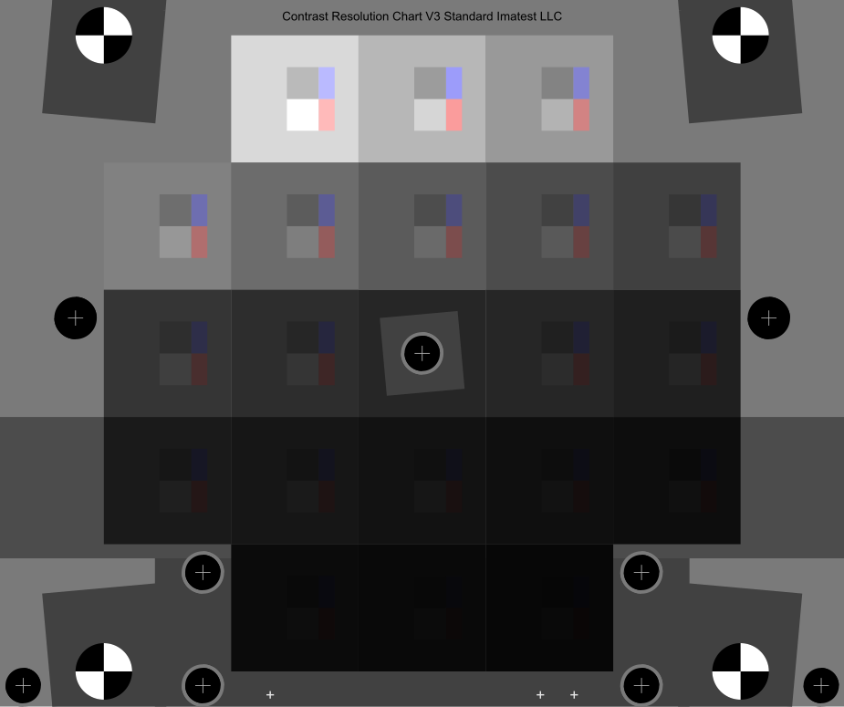
Here is a concept image (different from the actual chart, which has a range of tones too large to be reproduced on a web page).
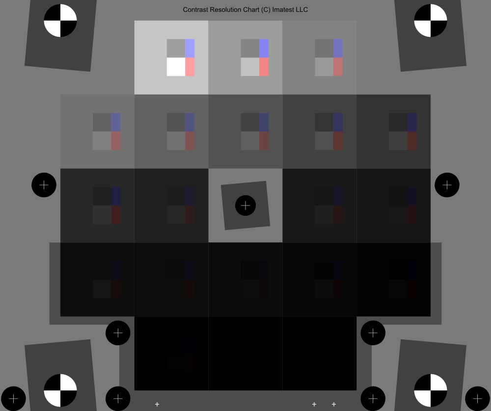 Contrast Resolution chart concept image
|
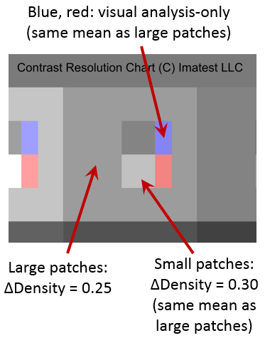
The physical Contrast Resolution Chart is made from two layers of 8×10 inch photographic film. It contains 20 large patches with Optical Densities (OD) ranging from base + 0.15 to base + 4.90 in steps of 0.25 OD (5 dB), equivalent to 95 dB*. (If the lightest and darkest small patches are included, the total density range is 5.05 OD = 101 dB.) The large patches are used for noise measurements because the small patches are usually too small for good noise statistics. *1 OD (optical density unit) = 20 dB (decibels) = 3.32 f-stops (or EV or Zones). Inside each large square (illustrated on the right) there are four small patches: light and dark gray, red and blue. The gray patches are 0.15 OD above and below the surrounding square. The difference, 0.30 OD (6 dB), is a 2:1 (simple) contrast ratio (100% Weber contrast). The mean density of the light and dark gray patches is identical to the density of the surrounding gray patch to minimize effects on tone mapping. (The same holds true for the blue and red patches.) The pixel levels of the small light and dark gray patches are used for a detailed quantitative analysis; the blue and red patches are used for a visual estimate-only). |
 |
|
Three contrast definitions are used in imaging literature. It’s important to know which one is used. Weber contrast: \(C_{Weber} = \frac{L_{max}-L_{min}}{L_{min}} = \frac{L_{max}}{L_{min}}-1 = 1\;\; (100\%)\) Simple contrast: \(C_{Simple} = \frac{L_{max}}{L_{min}} = 2\) Michelson contrast (modulation): \(Modulation = \frac{L_{max}-L_{min}}{L_{max}+L_{min}} = 0.333\) |
Many recent HDR image sensors claim a dynamic range of 120 to 150 dB. This may be the case for the sensor in isolation, but the dynamic range of real cameras with real optical systems isn’t even close. The practical limit is 100 dB at most, limited by flare light from bright areas inside or near the image field.
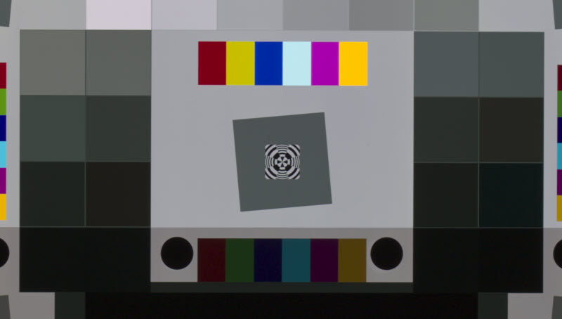
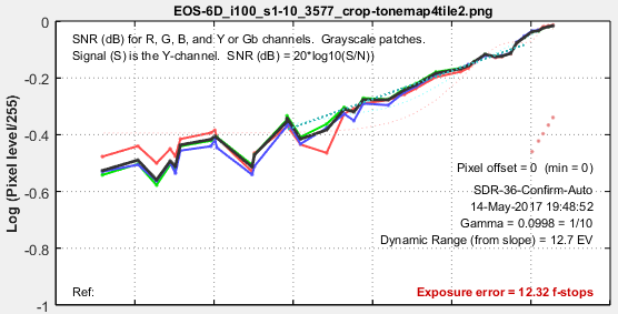
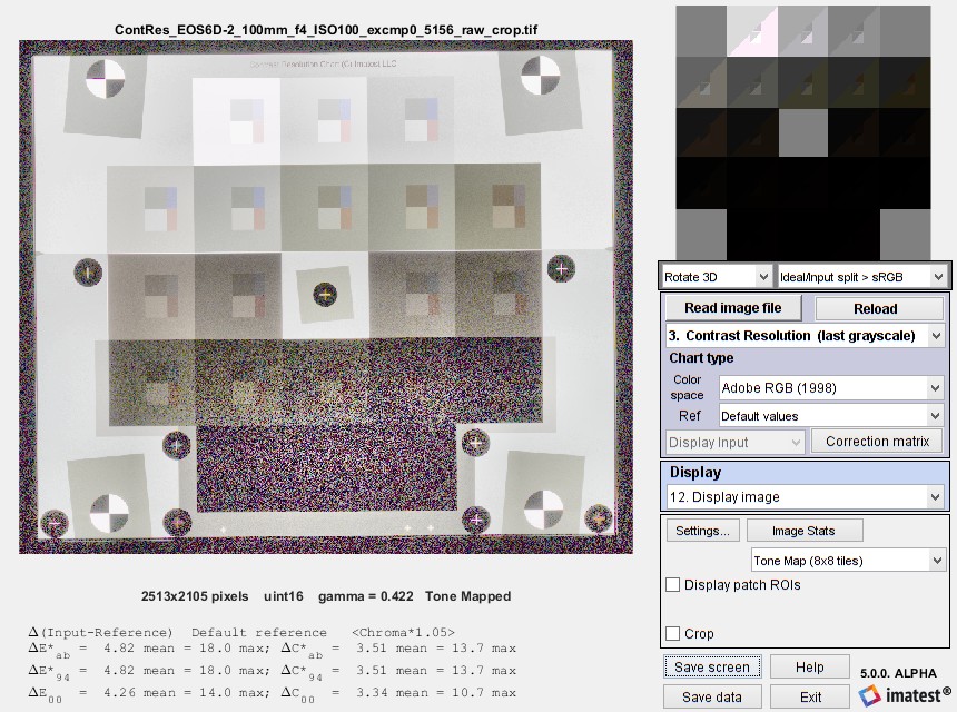
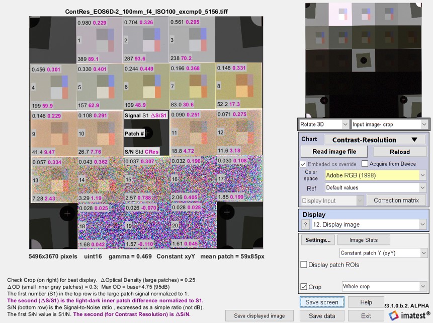
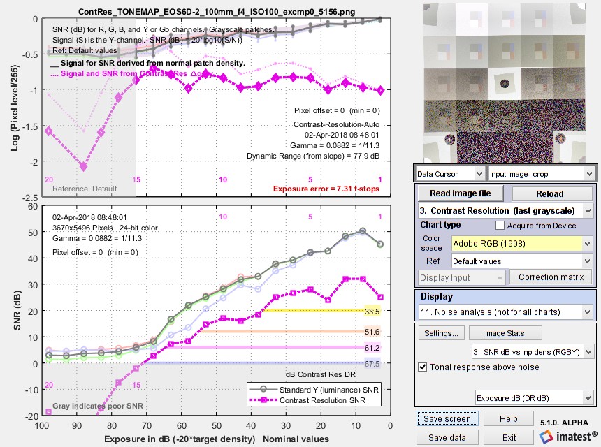
Here is an image of the chart taken by a Canon EOS-6D (a full-frame DSLR) with a high quality 100mm macro lens set to ISO 100, originally captured in raw format, converted to a DNG file (because LibRaw may not properly remove black level offsets (pedestals) from Canon CR2 files), converted to a 48-bit Adobe RGB TIFF file for analysis (with no sharpening or noise reduction), then cropped. The image below is an 8-bit JPEG derived from the very large 48-bit TIFF file.
 Contrast Resolution chart image, originally captured in RAW format.
Click on image to open a fill-sized image, which can be downloaded for analysis.
Photographing and analyzing the chart
The Contrast Resolution chart, which can be purchased from the Imatest store, is a two-layer 8×10 inch (20x25cm) transparency that needs to be back illuminated. Although any relatively uniform, non-flickering lightbox will work, we recommend the ITI Lightbox, which is extremely uniform (97%), can be dimmed over a wide range (300:1), and has two color temperatures (normally 3100 and 5100K, but other combinations can be custom-ordered).
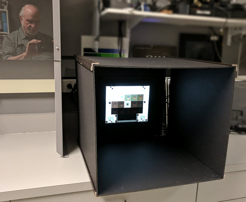 The chart should be photographed in a completely darkened environment. Care must be taken to avoid any light from reflecting back to the front surface of the chart. We ordinarily surround the light box with a box made from black foam board and corner molding to prevent local reflections. We are thinking of lining the box with blackout material to improve the light absorption. The area behind the camera should be as dark as possible. Light-colored clothing— which can reflect light back to the chart— should be avoided.
Test setup showing black box around the lightbox and chart
Pay no attention to that man behind the curtain.
Frame the chart so that the chart height in the image is at least 400 pixels— more is desirable for high resolution systems. In typical high resolution systems the chart should fill approximately 40% of the vertical or horizontal field. We recommend that you avoid filling the image with the chart because light falloff from the lens could reduce the measurement accuracy.
Analysis of the Contrast Resolution chart is included in the interactive Color/Tone Interactive and batch-capable Color/Tone Auto modules in Imatest 5.0+.
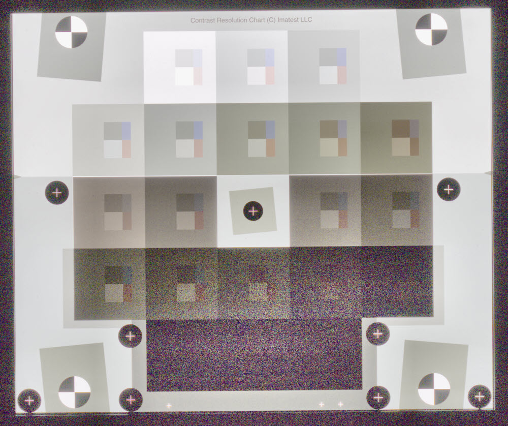
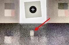 Reflections can be a serious issue. We recommend covering everything near the camera, except the lens, with black velvet or fleece. Reflections from the lens itself are hard to avoid, but their effects can be mitigated it by placing the camera so that its reflection is in the exact center of the image (for charts with circular layouts). This places the reflection outside of the density patches. In the image on the right, a reflection below the chart center spoils the measurement of patch 15. It’s easy to miss when taking the picture, but it can be painfully obvious when the image is viewed lightened (tone-mapped in this case). The camera needs to be raised slightly go get the reflection out of the density patches. Reflections can be a serious issue. We recommend covering everything near the camera, except the lens, with black velvet or fleece. Reflections from the lens itself are hard to avoid, but their effects can be mitigated it by placing the camera so that its reflection is in the exact center of the image (for charts with circular layouts). This places the reflection outside of the density patches. In the image on the right, a reflection below the chart center spoils the measurement of patch 15. It’s easy to miss when taking the picture, but it can be painfully obvious when the image is viewed lightened (tone-mapped in this case). The camera needs to be raised slightly go get the reflection out of the density patches. |
To run the image in Color/Tone Interactive,
- Click the Color/Tone Interactive button in the Imatest main window,
- Select 7. Multi-row Grayscale & Color charts from the dropdown menu just below the Read image file button.
- Select the image. This opens the Color/Tone Interactive Special Chart selection window.
- Select 13. Contrast Resolution.
- Reference source should be either Default values or a file name we can supply that contains the densities of the 20 large patches.
- Click OK.
For succeeding runs, you can simply click 3. Contrast resolution (last grayscale) in the Color/Tone Interactive window (this eliminates the Color/Tone Interactive Special chart selection) or Read image file if 3. Contrast Resolution… is displayed in the dropdown menu. You only need to press 7. Multi-row… if you are changing the chart type.
To run the image in Color/Tone Auto (the non-interactive, batch-capable version of Color/Tone Interactive, which should be run first to make sure settings are correct),
- Press the Setup button just to the right of Color/Tone… (middle-left of the Imatest main window).
- Chart type should be set to either 7. Multi-Row Grayscale... or 3. Contrast Resolution… (if the Contrast Resolution chart was used for the last run).
- Special (multi-row) grayscale chart type should be set to 13. Contrast Resolution.
- The only relevant plots are B&W Density & White Bal., Noise/SNR (two plots can be selected), and Image plot. (The others are all for color.)
- Click OK. Color/Tone: Contrast-Resolution will appear in the Imatest main window.
- Press this button to run Color/Tone. More details in the full Color/Tone instructions.
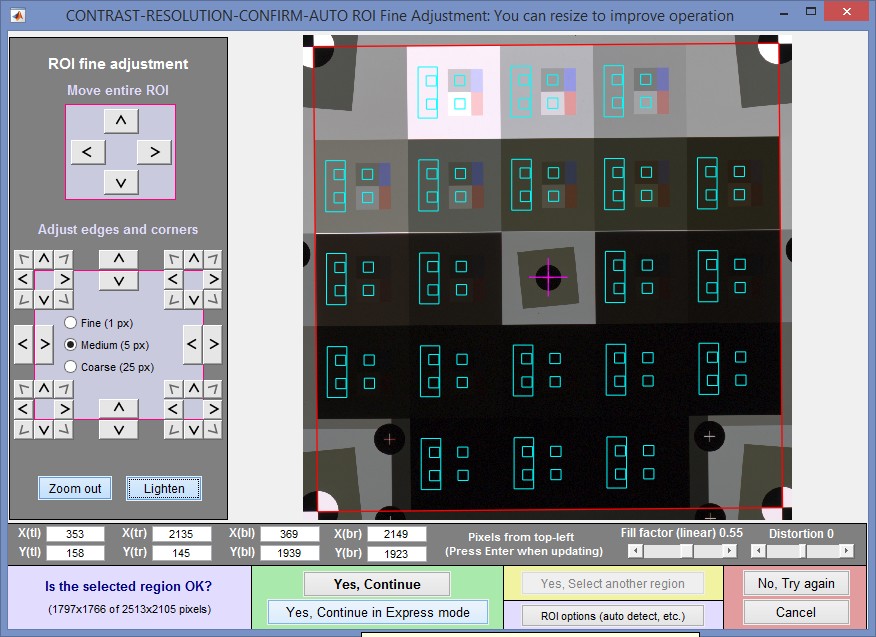
Chart detection is fully automatic when Auto detection for the 36-patch Dynamic Range and Contrast Resolution charts has been selected in ROI settings. Auto detection has become very robust (manual selection is also available). Here is the fine adjust window following automatic detection (or manual selection). If the adjustment is correct (distortion can be added if needed) click Yes, Continue in Express mode (or Yes, Continue). In Color/Tone Interactive, which is highly interactive, settings can always be changed later. (For Color/Tone, settings need to be made prior to the run.)
 Contrast Resolution fine adjustment window
Five regions are selected for each of the twenty large patches. The large rectangle is for the uniform gray area: if you’ve framed the image properly it should be large enough for good noise statistics. The two small rectangles to the right are for the dark and light gray areas. The two small squares inside the large rectangle are used to subtract the effects of vertical nonuniformity (due to flare light) from the light-dark gray patch measurement.
The Display settings of interest for the Contrast Resolution analysis are
7. B&W density & White Balance
11. Noise analysis
12. Display image
Results and Visualization
Tonal response and Signal-to-Noise Ratio (SNR)
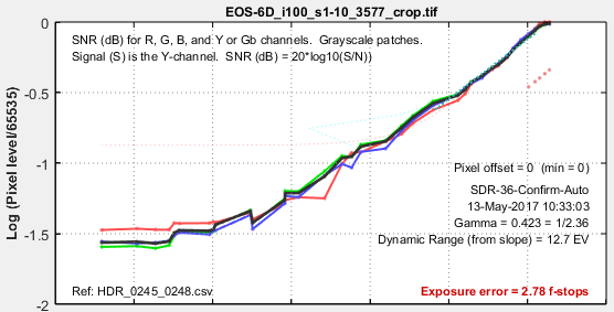
Here are the key results for tonal response and Signal-to-noise Ratio (SNR).
 Tonal Response and SNR for the 48-bit TIFF file derived from the RAW Canon EOS-6D image
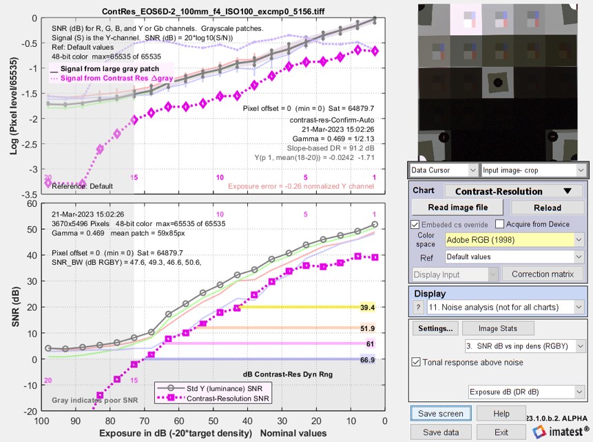
 Upper plot (log pixel level, i.e., tonal response) — The thin Red, Green, Blue, and Gray (for the Luminance (Y) channel) curves are from the large gray patches. They correspond to standard results for Dynamic Range charts. The small spikes in the gray curves (shown on the right) are the response for the light and dark gray patches within the larger gray patches.
The strong Magenta curve (– – – – –♦– – – – –) represents the difference signal ΔS = Slight − Sdark for the light−dark inner gray patches. This is a very good representation for the signal for determining the visibility of these patches. The weaker Magenta curve (– – – – –) is the difference signal normalized to the regular signal ΔS/Smid (the level of the large gray patch). The normalized difference signal stays relatively constant until patch 16, where is starts to drop abruptly.
|
The difference between the large gray patch response, Smid, and ΔS — a bit of math Let Rmid be the reflectance of the large gray patch. The light and dark gray inner patches (R1 and R2) are designed so their mean reflectance (R1+R2)/2 = Rmid and their ratio R1/R2 = 2. This is satisfied when \(R_1 = 4R_{mid}/3\) and \(R_2 = 2R_{mid}/3\). The image is encoded with an approximate encoding gamma (γ) curve, S ≅ Rγ, where for standard color spaces such as sRGB or Adobe RGB, γ ≅ 1/2.2 = 0.4545. Since the tonal response plot (above) has a logarithmic y-axis, what we really want is is log10 of the ratio between ΔS = S1–S2 and Smid. \(\Delta S/S_{mid} = (S_1-S_2)/S_{mid} = ((4R_{mid}/3)^{\gamma} – (2R_{mid}/3)^{\gamma})/R_{mid}^\gamma = (4/3)^\gamma -(2/3)^\gamma\) For encoding \(\gamma = 1/2.2 = 0.4545, \ \Delta S/S_{mid} = 1.1397-0.8317 = 0.3080. \) Finally, \(\log_{10}(\Delta S / S_{mid}) = \log_{10}(0.3080) = -0.5114 \) More generally, \(\Delta S/S_{mid} = \log_{10}((4/3)^\gamma – (2/3)^\gamma)\) This is the difference between the dark gray curve (Smid) and the Magenta curve for the contrast resolution signal Δgray = ΔS in the (upper) tonal response curve, above. This difference is displayed as a pale purple line that stays near -0.5 until it crashes around patch 16. |
Lower plot (Contrast Resolution SNR & Dynamic Range) — The strong Magenta curve (– – – – – with square markers) is the Signal-to-Noise Ratio derived from the light−dark gray difference signal ΔS. This is called the Contrast Resolution SNR, SNRCR *. The colored horizontal lines are the Contrast Resolution Dynamic Range, DRCR, described below. These are the most important results from the Contrast Resolution analysis. The plot background is gray where SNR drops below 0 dB (S/N < 1) to indicate that the image quality is too low for detail to be visible.
*SNRCR is a closely related to Contrast-to-Noise Ratio, CNR.
To make sense of these curves we need to look carefully at the image, and we need to deal with the poor visibility of the dark patches in most monitors under normal viewing conditions.
Visualization
A key attribute of the Contrast Resolution analysis is that it enables clear visualization of low-contrast objects within larger fields. This is not possible with standard grayscale charts with sequential patches.
|
One way patch contents can be visualized is by selecting Display image then selecting Tone Map (which applies the Matlab tonemap function) or one of the Constant patches options. Tone map (shown on the right) does not produce consistent results— it is affected by noise and minimum pixel level— but it’s of interest because the output of automotive cameras designed for human vision (Camera Monitor Systems) will almost certainly be tone mapped (though likely with more sophisticated routines). Tone mapping lightens the dark patches so that interior features can be visualized. It typically flattens the differences between large patches while maintaining contrast for the smaller inner patches. Tone mapped image (display-only): |
 |
Constant patches (available only in Color/Tone Interactive) provides a better display. The Constant patches display options (in the small dropdown window in the Settings region) have similar results.
- Constant patches (xyY) The image is converted in to xyY color representation, where Y is the (linear) luminance. This calculation uses the image Color space (typically sRGB, though Adobe RGB is occasionally used). The mean value of Y is calculated for each patch, then the entire parch is divided by mean(Y) and scaled for display. This typically gives the best display for color space images, but results are quite similar to Constant patches (simple).
- Constant patches (L*) The image is converted into CIELAB L*a*b* (using the image Color space). The mean value for L* is calculated for each patch and used to scale the image for constant mean L*. Patches in dark areas are typically undersaturated.
- Constant patches (simple) The mean value of each patch is calculated, then the entire patch is divided by the mean and scaled for display. No assumptions regarding color space or linearity are applied.
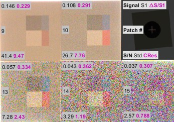
 Constant patch image (from Y in xyY): a good indicator of feature visibility.
Several numbers are shown in each patch this display. Here they are for a typical patch (#10).
| Line | Contents (patch #10) |
Description |
| 1 | S 0.108 0.291 |
The first entry in patch #10 (S1 = 0.108) is the signal for the patch normalized to 1.0. The second entry (ΔS/S1 = 0.291) is the difference between the small light and dark gray patches inside the larger patch, normalized to the signal (S1) in the first entry. Log10(S1) and log10(ΔS/S1) are displayed in the upper plot of the Tone and Noise (or SNR) figure. Log(0.291) = -0.536. This is the difference between the large gray patch signal and the Contrast Res Δgray signal. |
| 2 | 10 | Indicates the patch number (10) |
| 3 | 26.7 7.76 |
Signal-to-Noise Ratios. Noise N is calculated in the large patch. The signal for the first SNR (SNR(S)) is the mean pixel level of the large patch (S1 in line 1). The signal for the second SNR (SNR(ΔS) = SNRCR) is the difference between the small light and dark patches, ΔS. This number relates to how well the two gray patches with 2:1 (100% Weber) contrast can be distinguished. SNR(S) and SNRCR are displayed logarithmically (as simple ratios or dB) in the lower plot of the Tone and Noise (or SNR) figure (——— and – – – – –, respectively). SNRCR is closely related to Contrast-to-Noise Ratio (CNR). |
Visual analysis
By comparing the Constant patch image with the Tonal Response/SNR plots above we can learn quite a lot about Contrast Resolution.
From the above Constant patch image we make a preliminary observation.
- The inner patches are clearly visible to patch 13, where SNRCR = 2.43.
- The inner patches are weakly visible and noisy in patch 14, where SNRCR = 1.19.
- The inner patches are difficult to see (visible only because they resemble patches in regions with better SNR) in patch 15.
- The inner patches are invisible in 16 and beyond.
Note that the normalized signal ΔS/S1 stays fairly consistent through patch 16, and only seriously drops for patches 15 and beyond. This is a pretty clear indicator that the normalized signal is not a good indicator of performance. Contrast Resolution SNR, SNRCR is much better.
Contrast Resolution Dynamic Range
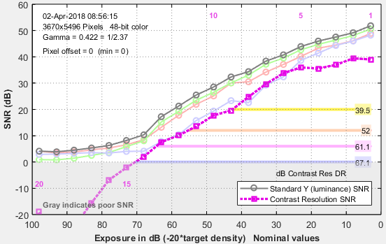
Illustration of Contrast Resolution Dynamic Range, based on SNRCR
Contrast Resolution SNR (SNRCR) can be used as the basis for defining a Contrast Resolution Dynamic Range (DRCR) — the range of tones over which the SNR and/or signal stays above specified values. The light and dark DRCR limits are defined differently because noise is very low for the light patches, hence signal-only is used.
Dark DRCR limit is the minimum exposure where SNRCR is in the range of 6 to 12 dB (2:1 to 4:1) for good visual discrimination. DRCR is defined using the same SNR levels used for standard Imatest Dynamic Range calculations, 20, 12, 6, and 0 dB (S/N = 10, 4, 2, and 1) for “High”, “Medium-High”, “Medium”, and “Low” quality levels, respectively. (These designations are somewhat optimistic.)
The value of SNR used to define the dark DRCR limit can be adjusted for specific applications. For example, if a lower contrast feature were of interest, the SNR value for calculating DRCR (based on the chart image) could be increased.
Light DRCR limit is maximum exposure that excludes saturated regions, where contrast is too low for good visual discrimination. It is based on two signal differences for each large patch: ΔSLM = Slight – Smiddle and ΔSMD = Smiddle -Sdark , where middle denotes the large middle gray patch and light and dark denote the small light and dark patches, respectively. The algorithm is
- Find the maximum value of ΔSLM and ΔSMD for all patches. Call these values ΔSLM(max) and ΔSMD(max).
- Starting with the lightest patch, find the first patch where either (A) ΔSLM ≥ 0.1*ΔSLM(max) or (B) ΔSMD ≥ 0.1*ΔSMD(max).
- If both conditions (A) and (B) are met, the upper DRCR limit is the exposure corresponding to the patch.
- If only one condition ((A) or (B)) is met (it will typically be (B)-only), the upper DRCR limit is the mean of the exposures for current and next patch. This is typically about 2.5 dB lower than the current patch (for a nominal 5 dB patch difference).
Finally, DRCR = Light DRCR limit – Dark DRCR limit Shown as 4 horizontal lines in the above plot: –– –– –– –– .
A paper, “Signal-to-noise optimization of medical imaging systems” by I.A. Cunningham and R. Shaw, describes a measurement called SNRRose similar to this SNRCR and indicates that a value of 5 or greater is required for reliable detection of an object. From looking at these results it appears that a lower SNRCR as low as 2 might be sufficient (though marginal), at least for 2:1 contrast patches. More work needs to be done to determine a good lower limit, which is very likely to be close to the value of 5 from the paper. We recently discovered Wikipedia pages describing Contrast Resolution and Contrast-to-Noise Ratio (CNR) that lack practical measurement methods.
Tone mapped results
|
It is instructive to look at results for a tone mapped image. To obtain such an image we applied the Matlab tonemap tone mapping algorithm with the default value of 8 tiles to the above image using the Imatest Image Processing module. Tone mapped image, derived from above image, The tone curve in the upper plot (below) is very different from the original image. The tonal response has been flattened so that the gamma (the average slope in gray regions) has been reduced from 0.422 to 0.0734— a meaninglessly low value. But the normalized light-dark gray difference signal ΔS/S (the thin dashed Magenta line: – – – – –) and the light-dark gray difference Signal-to-Noise Ratio ΔS/N (the strong Magenta curve – – – – – with square markers) in the lower plot are fairly close. |
 |
These results clearly show that Contrast Resolution measurements— especially the difference-based Signal to Noise Ratio ΔS/N— are affected very little by tone mapping, i.e., good measurements can be made in tone mapped systems.
 Tonal Response and SNR for the tone mapped image derived from the RAW Canon EOS-6D image
The reason that noise and SNR are relatively stable when tone mapping is applied is that the Imatest noise calculation is quite robust against nonuniform illumination within regions of interest— created by tone mapping. Noise is ordinarily equivalent to the standard deviation (σ) of the levels in a smooth (flat) region, but this simple calculation can misinterpret nonuniformity as noise. Imatest subtracts a second-order fit to the mean horizontal and vertical pixel levels from the region prior to calculating noise— effectively removing nonuniformity from the calculation. The difference between the simple and nonuniformity-corrected calculations can be observed by running the Imatest Image Statistics program.
Flare mask and two-image flare measurement
In 2021.2 we have added support for a flare mask, which greatly reduces the flare in Contrast-Resolution chart measurements, enabling two Dynamic Range measurements (representing normal and low flare) as well as a flare (veiling glare, i.e., stray light) measurement from two images. An image of the mask, which fits tightly in the frame that holds the chart, is shown on the right, below. The circular openings (for the registration marks) are covered by neutral density gel filters with an optical density of 1.2 to minimize flare and (in most cases) allow automatic region detection. Autoexposure should not be used for this method: most autoexposure algorithms cause the brightest patches to become overexposed, sometimes severely. Manual exposure control is strongly recommended. The exposure should be set (if possible) so the lightest regions of patch 1 (the inner square and the outer background) are saturated, but the darker inner square is not.
 Contrast Resolution concept chart Contrast Resolution concept chart |
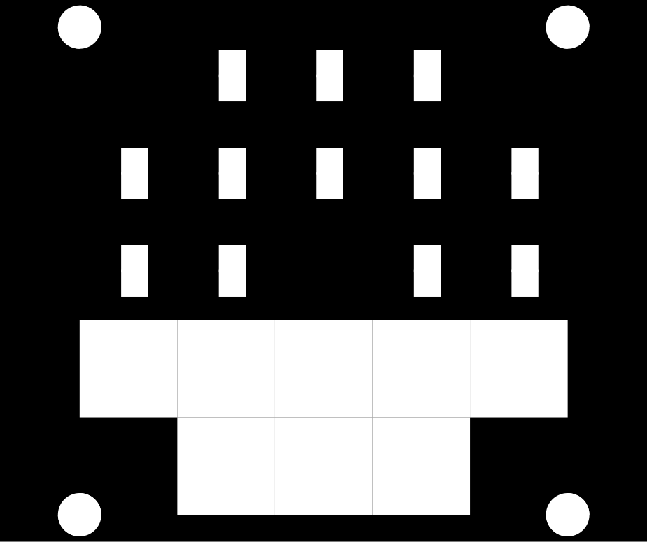 Contrast Resolution flare mask Contrast Resolution flare mask |
When the image is masked, the signal normally calculated from the left side each patch is replaced by the average of the two smaller (lighter and darker) squares, and the noise is calculated from one of the two squares (the lighter square, except for the top row). Most of the results are similar with and without the mask, except for one major difference. The flare is greatly reduced with the mask, which may increase the Dynamic Range, but most importantly, the mean of log pixel levels in the bottom row (patches 18-20), which are closely related to flare light, is reduced. The flare measurement is the difference in the log pixel levels in the bottom row measured without and with the mask.
More details can be found on Veiling Glare AKA lens flare.
Summary
We have shown that the Contrast Resolution chart produces a clear indication of the visibility of low contrast objects (using small patches with a 2:1 transmittance ratio (a 0.3 Optical Density difference; 100% Weber contrast) inside larger squares). Unlike standard grayscale step charts, it works well with tone mapped images and is insensitive to errors caused by flare light and uncompensated black level offset.
Contrast Resolution SNR = SNRCR = ΔS/N, which is based on the light-dark patch difference, provides an excellent indication of the visibility of the light and dark objects of similar contrast. When SNRCR is larger than a value in the range of 2 to 4 (6-12dB)) the objects can be effectively distinguished.
 This criterion has been used to establish a set of Contrast Resolution Dynamic Range DRCR measurements, which are defined as the range of scene brightness (exposure) where small objects with a OD difference of 0.3 have SNRCR > n, with n = 10, 4, 2, or 1 (20, 12, 6, or 0dB). 10 is “high” quality; 1 is low quality, where objects cannot be distinguished. n is in the range of 2 to 4 for distinguishable objects.
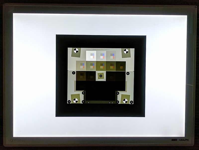
Contrast Resolution chart on a 17×24 inch Artograph Lightpad
for alternative veiling glare measurement
The Contrast Resolution chart could also be mounted (preferably without a frame) on a large lightbox, such as the 17×24 inch Artograph Lightpad, to measure veiling glare, which would be indicated by the measurement difference (the difference in SNR(ΔS)) between images without and with the light surround.
Verification
The darker patches in the images used in this page contain no visible detail in images we’ve acquired. This naturally leads to the question, is detail present in the charts themselves? This took some effort to verify. What we did is to mask off all but the bottom two rows of the chart (to minimize fogging from flare light), then acquire some images. Here are the results showing that the darkest patches do indeed contain detail.
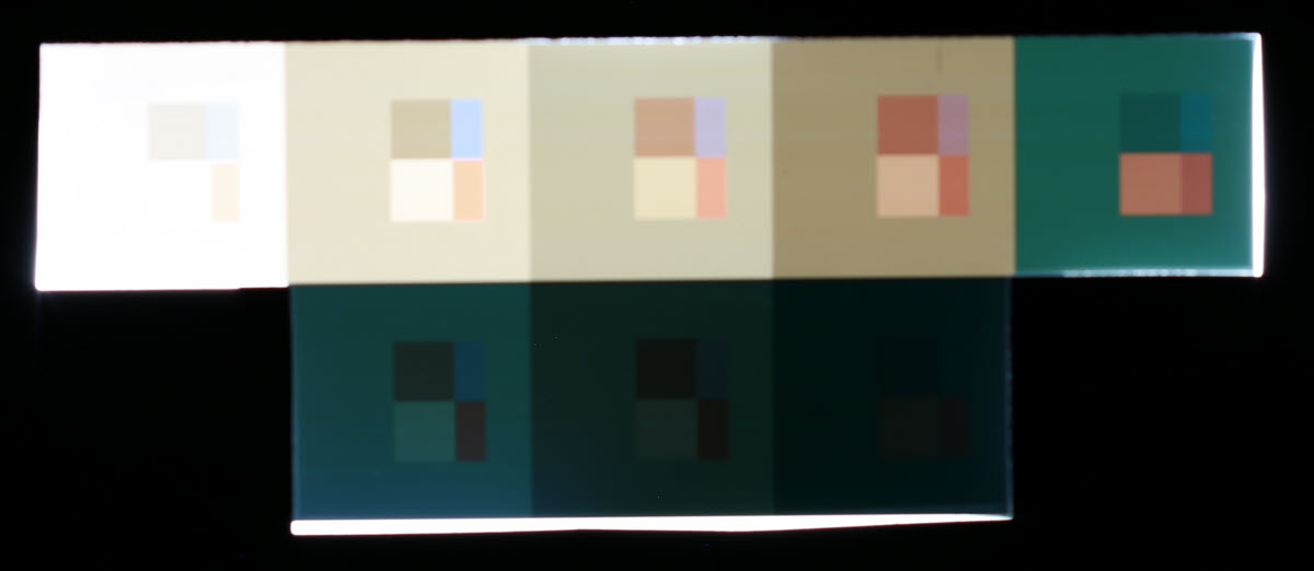 Bottom two rows (with others masked), Normal exposure
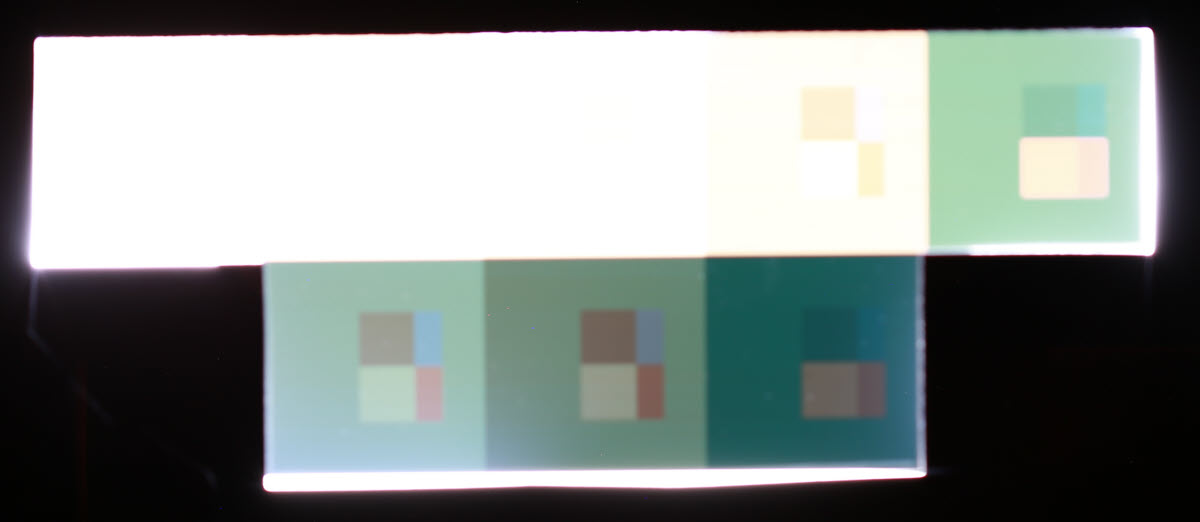 Bottom two rows (with others masked), Extreme overexposure
Note some unevenness from flare light (from the thin unmasked strip) is visible in the bottom row.
These images clearly show that information is present in the darkest patches. some discoloration is noted. This comes from our process, which has some issues in very dark patches. It has little effect on the results, and is not visible in patches bright enough to be visible in normal viewing conditions.
Reference
F. Timischl, The Contrast-to-Noise Ratio for Image Quality Evaluation in Scanning Electron Microscopy,
JEOL Technics Ltd., 2-6-38 Musashino, Akishima-shi, Tokyo, Japan (can be read online; difficult to download) Contrast Resolution SNR is closely related to CNR.