Gamutvision main page – Gamutvision Table of Contents/Site map – Using Gamutvision – Using Gamutvision 2: Displays
There is a significant difference between a printer’s total (maximum) gamut and the achievable gamut when printing from a working color space. With Gamutvision you can display both and compare them side-by-side. You can also compare the gamuts available from different working color spaces.
|
To see how the difference is displayed, let’s review Gamutvision’s data flow. The total gamut of a device is obtained when its ICC profile is used as an input profile, i.e., one of the RGB gamut patterns (RGB input) is mapped to device-independent L*a*b*, xy, or uv using the profile. The total gamut for a device (i.e., printer, monitor) profile can be obtained by
|
 |
|
This broader picture of Gamutvision’s structure illustrates the display possibilities. You can select up to four ICC profiles: two input profiles and two output profiles.
|
 |
You might, for example,
- Enter a printer profile into Profile 1. The profile 1 display will contain the total gamut.
- Enter a working color space profile into Profile 3 and the (same) printer profile into profile 4. The gamut actually achieved (with rendering intent 3→4) is displayed as Profile 4.
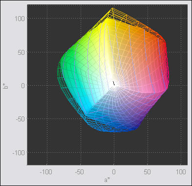
- Display Profiles 1 and 4 simultaneously using Display A or Display B. This is shown below. The display is 3D L*a*b* (wire input, solid output). has been pressed. ( is shown in its place.) so the a*b* gamut is displayed. Results are shown below.
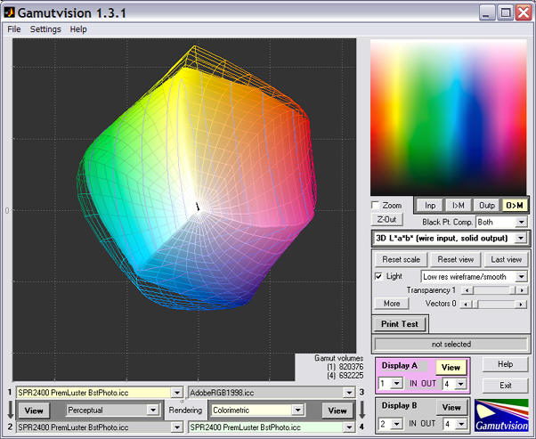
Mapped (solid) vs. total (wireframe) gamut
The gamut volumes are displayed on the lower-right of the image. The volumes are 820,376 for the unmapped profile and 692,225 for the profile mapped from Adobe RGB.
For clarity, the background color has been set to 0.2 using the button. Clicking enlarged the gamut image from its normal (small) size. You can also enlarge the gamut image by clicking , then selecting a value for 3D plot axis setting other than the default vis3d. Although the image will be larger, the a*b* axes may not display properly.
For example, to compare the effects of two working color spaces with a single printer/profile combination, you would enter the two working color space profiles into input Profiles 1 and 3 and the same printer profile into output Profiles 2 and 4. You could then view profiles 1 and 2 or 3 and 4 (showing the effects of the gamut mapping), or you could use Display boxes A or B (shown above) to compare the output gamuts in profiles 2 and 4. The gamuts for Epson R2400 Premium Luster prints made from Adobe RGB (1998) (wireframe) and sRGB (solid) working color spaces are shown on the right, using the 3D L*a*b* display set to . The gamut volumes are 698,960 and 562,168, respectively; the volume is 24% larger when mapped from Adobe RGB. (Displays on this page use Epson-supplied X-rite “premium” profiles, released around October 2005; different from earlier profiles supplied with the R2400). |
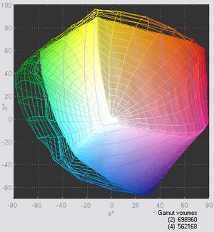 Mapped gamuts from sRGB (solid), and Adobe RGB (1998) (wireframe) |
Caution:
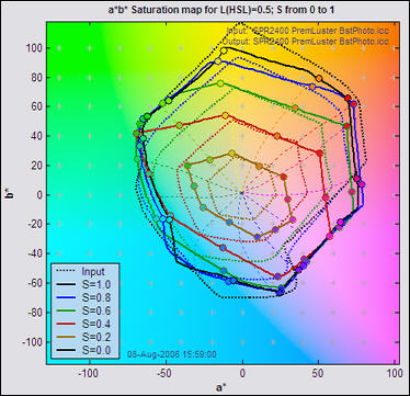
To see the entire gamut of a printer profile you should always use the 3D L*a*b* view, set for Top view. You should never use the 2D a*b* Saturation view, which works well for color space profiles or mapped printer profiles, but does not work well when a printer profile is used as an input profile or an output profile with Rendering set to None. The reason: The 2D a*b* Saturation map is based on a gamut image where L(HSL) = 0.5. (This is L in the HSL color representation, not L*.) In normal color spaces, colors have their maximum saturation where L(HSL) = 0.5. But printers are highly nonlinear devices: they don’t necessarily reach maximum saturation at for L(HSL) = 0.5; hence the 2D a*b* saturation map can produce the strange result shown on the left, which is not the true device gamut.
|
Mapped vs. total gamuts (displayed incorrectly (left) and correctly (right))
|
|
|
|
 3D L*a*b* (top view): correct |
|
Comparing the gamut of Adobe RGB (1998) mapped with (relative) colorimetric rendering intent
to Epson R2400 Premium Luster (output profile) to the total gamut of Epson R2400 Premium Luster (input profile) |
|
Real-world images and color spaces
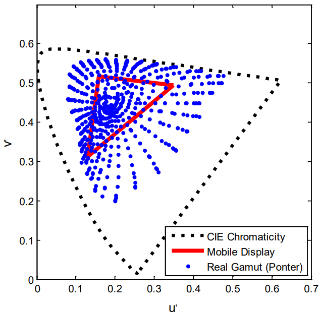
In the presentation Metrics for Comparison of Color Encodings (CIE TC8-05) by Kevin Spaulding and Gus Braun of Kodak, formerly available online from colour.org, the authors have created a CIE xy diagram representing the full range of colors available from reflective surfaces. They used a wide variety of sources (graphic arts spot colors, etc.) to assemble this diagram (slide 5 in the presentation). Their results are similar to the Pointer’s gamut, which hard to find on the internet. It is instructive to compare their results to the two best known color spaces, sRGB and Adobe RGB (1998).
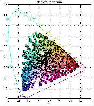 xy Real-world reflective colors xy Real-world reflective colorsuv Pointer’s gamut colors |
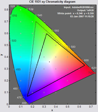 xy Adobe RGB (dotted), sRGB (solid) xy Adobe RGB (dotted), sRGB (solid)u’v’ Adobe RGB (S = 1, 0.8, 0.6, …) |
 from Color.org
|
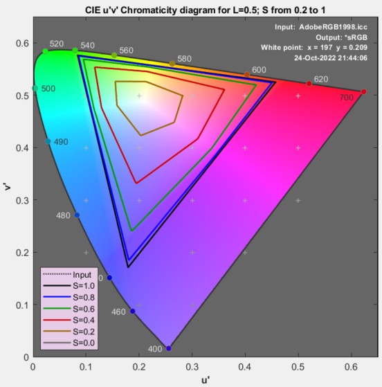 |
Although the eye can see more highly chromatic colors than these (represented by the outer horseshoe), they are extremely rare in nature. The best examples are the vibrant colors of a prism in the sun and some rare irridescent butterflies (generated by optical interference)— colors that can’t be reproduced by standard output devices (monitors or printers). Adobe RGB (1998) encompasses most of the reflective colors; only a few reds and cyans are out of gamut, and not by much. The eye is not extremely sensitive to chroma differences in highly saturated colors. So Adobe RGB is a safe, conservative choice for a working color space. sRGB is clearly weaker in greens and cyans. It’s the standard color space of Windows and the internet— by far the most convenient, foolproof choice , but Adobe RGB is preferred when the intended output is high quality inkjet prints.
The reader is cautioned that the CIE 1931 xy chromaticity diagram has several well-known limitations. The space occupied by the greens is exaggerated, and the 2D representation has no information on the lightest or darkest colors.