Chromatic Aberration, noise, and Shannon capacity plot details
The camera chosen for the plot below has significant Chromatic Aberration. The Noise spectrum and Shannon capacity plots, shown below beneath Chromatic Aberration, are plotted only if the Noise Spectrum and Shannon capacity (in CA plot) checkbox in the Imatest SFR input dialog box has been checked. It is unchecked by default.
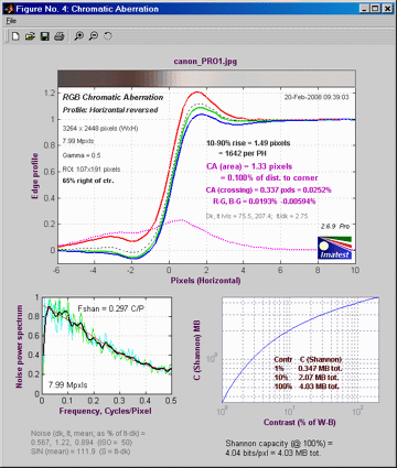
Upper plot: Chromatic Aberration |
||||||||
| More about this plot can be found in the page on Chromatic Aberration. Much of this plot is grayed out if the ROI is too close to the center for reliable CA measurements (less than 30% of the distance to the corner). |  |
|||||||
| Red, Green, and Blue lines (bold) |
Edge profiles for the R, G, and B channels (original, uncorrected). (Standardized sharpening is not used for chromatic aberration.) | |||||||
| Black line (dashed) | Edge profile for the luminance (Y) channel. | |||||||
| Dashed magenta line (bold) |
The difference between the highest and lowest channel levels. (All channels are normalized to go from 0 to 1.) The visible chromatic aberration is proportional to the area under this curve. | |||||||
| Left column text |
Input settings: Plot title, profile orientation (Horizontal profile corresponds to a vertical edge, etc.), image dimensions (WxH), total megapixels, gamma, ROI size, ROI location. | |||||||
| Right column text
(results) |
|
|||||||
| Below the plot |
These items are only displayed if the Noise Spectrum and Shannon capacity box is unchecked. Noise in the dark and light areas, described below. A thumbnail of the image showing the region of interest (ROI). |
|||||||
Noise and Shannon information capacityLower part of figure: Noise and Shannon information capacity plots for for the selected channel, normally luminance (Y)Shannon capacity is an experimental measurement that is strongly affected by signal processing (especially sharpening and noise reduction). It is not a reliable way of quantifying camera performance (though it’s better with RAW files than with processed files (in-camera JPEGs)). |
||
| Noise spectrum plot (left side) |
The noise spectrum plot is somewhat experimental. Bayer interpolation causes the noise spectrum to roll off to about 0.5 at 0.5 Cycles/Pixel; noise reduction causes additional rolloff. Low to middle frequency noise components tend to be more visible. The spiky light cyan and green curves represent two different directions. The thick black line is the smoothed average of the two. The red line is a third order polynomial fit to the noise. | Noise spectrum and Shannon capacity are only plotted if the selected region is large enough to provide reasonable noise statistics. 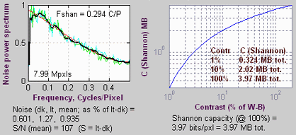 |
| Shannon capacity plot (right sde) |
Shannon capacity C as a function of signal S (closely related to image Contrast), where S is expressed as the percentage of the difference between the white and black regions of the target (Sstd ). A Contrast of 100% represents a fairly contrasty image, 10% represents a low contrast image, and 1% represents a smooth area like skies. These numbers are only meaningful for comparing digital cameras. They should be used with caution because signal processing, especially noise reduction, has a strong effect on Shannon Capacity. There is a table of results in the page on Shannon information capacity. | |
| Text at bottom |
Noise in the dark and light areas, and the mean of the two. Measured after the input data has been linearized (corrected for the gamma encoding). Expressed as a fraction of the difference between the average levels of the light and dark areas (Sstd ). This difference is the standard signal, S, used in the calculation of Shannon information capacity. The noise measurements in Q-13 Stepchart and Colorcheck are more reliable and useful. Signal-to-noise ratio S/N for the mean of the light and dark areas. This is the inverse of the noise for the mean of the light and dark areas, above. Used in the calculation of Shannon capacity. Shannon information capacity of the camera for signal S = Sstd, measured in bits per pixel and megabytes total. This is an approximate calculation that provides an estimate of overall image quality for moderately contrasty images, as affected by sharpness and noise. |
|