NOTE: This will be deprecated in a future release
Auto-exposure – Saving – Dynamic range (DR) – DR definitions – Algorithm
Stepchart measures the tonal response, noise, dynamic range, and ISO sensitivity of digital cameras and scanners using
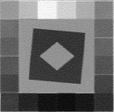
- Reflective grayscale step charts such as the Kodak Q-13 and Q-14 Gray Scales, which have a single row of patches (a linear arrangement), or charts such as the ISO-14524 or ISO-15739 charts, with non-linear (multiple rows; may be circular) patch arrangements, shown below, or
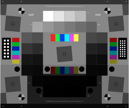
- Transmissive (backlit) grayscale step charts such as the Imatest 36-patch Dynamic Range or 36-patch High Dynamic Range chart, as well as charts from Stouffer, Kodak, DSC Labs, and Danes-Picta. Transmissive charts, which have higher maximum densities than reflective charts, can be used to measure dynamic range from a single image.
Stepchart can also measure veiling glare (susceptibility to lens flare).
| Most Stepchart functions are now included in Color/Tone Setup and Color/Tone Auto; a fixed; batch-capable module with identical calculations to Setup). Both are newer and offer a greater selection of results plots and noise and dynamic range analyses. These modules are recommended for new work. |
| News: Nonuniformity correction, long-available, has been documented. Imatest 5.1 (starting December 2018) The exposure error calculation has been improved to be more consistent over a range of contrast (gamma) values. Details here. Imatest 5.1 ALL Stepchart functions including temporal noise are now included in Color/Tone Auto. Most were included in Imatest 4.0. Stepchart chart type can be selected prior to running Stepchart with Stepchart Chart Selection (in the Settings dropdown menu). Automatic region detection is supported with the 36-patch Dynamic Range, ISO 14524 (with registration marks) and ISO 15739 (with registration marks) charts. |

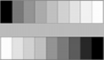
Stepchart was originally written for the Kodak Q-13 and Q-14 Gray Scales are inexpensive 8 and 14 inch long charts consisting of 20 zones, labeled 0-19, which have optical densities from 0.05 to 1.95 in steps of 0.1 (reflectance from 0.891 to 0.011). The charts are printed on a luster (semigloss) surface. The Q-13 image on the right was photographed very slightly out of focus to minimize noise from chart texture.
Additional (multiple-row or circular) charts for Imatest Master
Several monochrome targets, shown below, can be analyzed with Imatest Master. To run them, open the image file, then select the approximate region of interest for the key features in the target, following the instructions in Stepchart with Special/ISO targets. Additional dialog boxes allow you to specify the target type and refine the crop.
 QA-61 ISO- 16067-1 Scanner |
 QA-62 |
 ST-51 EIA Grayscale |
 ST-52 ISO- 14524 12-patch OECF target |
 ISO-15739 Noise target |
|
Imatest 36-patch |
 20-patch OECF targets |
 ITE Grayscale |
 SFRplus 20-patch stepchart |

Photographing the chart
- Light. Be sure the light is uniform and free of glare. Lighting uniformity can be measured with an illuminance (Lux) meter. A variation of no more than ±5% is recommended. If possible, the surroundings of the Step chart should be gray or black to minimize flare light (unless you are measuring flare light). An 18% gray surround is recommended for cameras with auto-exposure.
- For reflective charts, as little light as possible should come from behind the camera— it can cause glare and flatten image tones. At least two lamps with an incident angle of about 20-45° are recommended. Lighting recommendations can be found in Building a Low-Cost Test Lab. Be especially careful to avoid glare in the dark zones on the right of the Q-13/Q-14 charts; it can hard to avoid with wide angle lenses. The light should not emphasize the texture of the chart, which would cause erroneous noise measurements.
- For transmissive charts, as little stray light as possible should reach the front of the chart. Use black curtains if needed.
- Focus. The chart may be photographed slightly out of focus to minimize noise measurement errors due to texture in the patches. Slightly is emphasized— the boundaries between the patches should remain distinct.
- Distance. Distance is not critical. The width of the chart image should be no more than about 2/3 of the total image width to minimize vignetting (light falloff, which can be serious with wide-angle lenses). The noise analysis will be most accurate if each patch is 50 pixels wide, but fewer are adequate for low resolution cameras. Increasing the size improves the accuracy of the noise measurement up to a point, but there is little improvement for patches over 100 pixels wide. Tonal response can be measured with very small images, as long as the zones are distinctly visible.
- Photograph the chart.
- Save the image as a RAW file, TIFF, or high quality JPEG, then load it on your computer. Raw images can be converted using dcraw (for commercial files) or Read Raw (for binary files). If you are using another RAW converter, convert to JPEG (maximum quality), TIFF, or PNG.
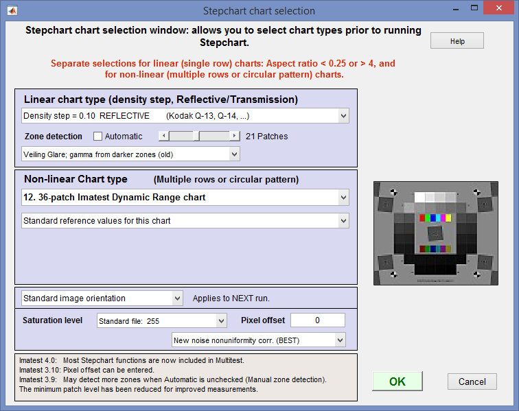
Stepchart chart selection window
Running Stepchart
- Run Imatest.
- Stepchart setup may be simplified by clicking Settings (dropdown menu in the Imatest main window), Stepchart selection… This opens the Stepchart chart selection window (shown on the right) that lets you select chart types for linear (single-row) or non-linear (multiple-row) charts prior to running Stepchart. This can be helpful with automatic region detection.
- Click on the button in the Imatest main window.
- Open the input file using the dialog box. Imatest remembers the directory name of the last input file opened (for each module, individually).
Multiple file selection Several files can be selected in Imatest Master using standard Windows techniques (shift-click or control-click). Depending on your response to the multi-image dialog box you can combine (average) several files or run them sequentially (batch mode).
Combined (averaged) files are useful for measuring fixed-pattern noise (at least 8 identical images captured at low ISO speed are recommended). The combined file can be saved. Its name will be the same as the first selected file with _comb_n appended, where n is the number of files combined.
Batch mode allows several files to be analyzed in sequence. There are three requirements. The files should (1) be in the same folder, (2) have the same pixel size, and (3) be framed identically. For the first image the settings window is identical to standard non-batch runs. Additional runs use the same settings. Since no user input is required they can run extremely fast.
Temporal noise (noise representing the difference between images) can be measured by selecting 2 files of identical (but separately acquired) step chart images, then selecting Read two files for measuring temporal noise in the Multi image file list dialog box.
One caution: Imatest can slow dramatically on most computers when more than about twenty figures are open. For this reason we recommend checking the Close figures after save checkbox, and saving the results. This allows a large number of image files to be run in batch mode without danger of bogging down the computer.
- Crop the image. The crop aspect ratio determines whether the analysis is for a linear (single-row) or nonlinear (multiple row) chart. For linear charts, the Zone detection setting shown below determines how regions are selected, and hence how you crop.
- When Automatic is unchecked (or for nonlinear charts), small blue rectangles for each of the patches will be displayed in the Fine Adjustment window, i.e., you immediately see the selected regions. For linear charts you need to enter the number of patches.
- When Automatic is checked, the patches are located automatically: no rectangles are shown during the region selection. Because this can cause problems in noisy images and dark regions, we recommend leaving Automatic (zone detection) unchecked.
- To measure veiling glare, Automatic must be unchecked. Make the appropriate selection in the dropdown menu on the right and select 21 regions (for the Q14) (the total grayscale patches plus one).

|
Typical crops (for Automatic zone detection are shown on the right, indicated by red rectangles. The orientation does not need to be correct; Imatest will rotate the image to the correct orientation. To display the exposure error correctly (reflective targets only), select the entire chart, including any clipped highlight patches that may be present. If the aspect ratio (length / width) of the crop is less than 4:1, a settings window for one of the nonlinear (multiple-row or circular) charts will appear (for Imatest Master and IS). If you plan to use manual Zone detection (selected in the Stepchart input dialog box, below), the selection can be approximate: a Fine adjustment window will open after the Stepchart settings window to enable you to refine the crop. |
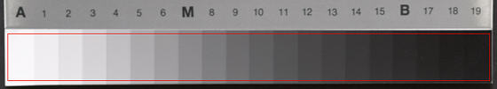 Crop of a Kodak/Tiffen Q-13 chart |
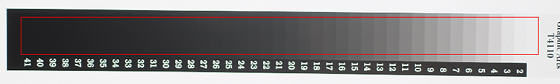 Crop of a Stouffer T4110 chart (better without the tilt). |
- Make any needed changes to the Stepchart settings box.
Stepchart settings
| You can select either Expert or Simplified mode for the settings window. In Simplified mode many settings are grayed out so they can’t be set. If you press , commonly used settings (recommended for beginners) are selected. |
Title Defaults to file name. Feel free to add useful descriptive material.
Chart type A reflective target with density steps of 0.10 (the Q-13/Q-14) is selected by default. If you are using a transmission target, be sure to choose the correct target type. In Imatest Master and IS you can enter a table of densities from an text file (one density per line) or a CGATS file (which may contain densities of L*a*b* values). Automatic (default) must be unchecked to enable Veiling glare measurements. (See Dynamic range, below.)
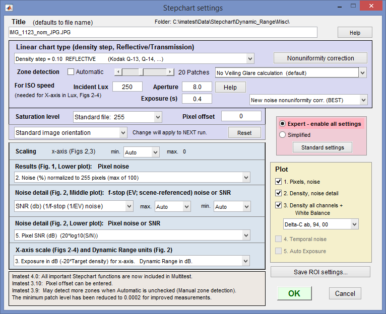
Stepchart settings window
Nonuniformity correction (available since Imatest 3.9) allows you to correct for nonuniform illumination using a separate flat field image taken under identical conditions. Opens the Nonuniformity correction window described in Nonuniformity Correction in grayscale and color chart modules.
Zone detection For linear (single-row) charts you select either Automatic or Manual Zone detection with the Automatic checkbox. If Automatic is unchecked, select a fixed number of patches (6-41) with the slider for Stepchart analysis, and a fine ROI adjustment box appears after is pressed. This option is useful when there is high noise in dark regions or when veiling glare is to be calculated. (Zone detection can also be set from in the Imatest main window.) We strongly recommend leaving Automatic (zone detection) unchecked.
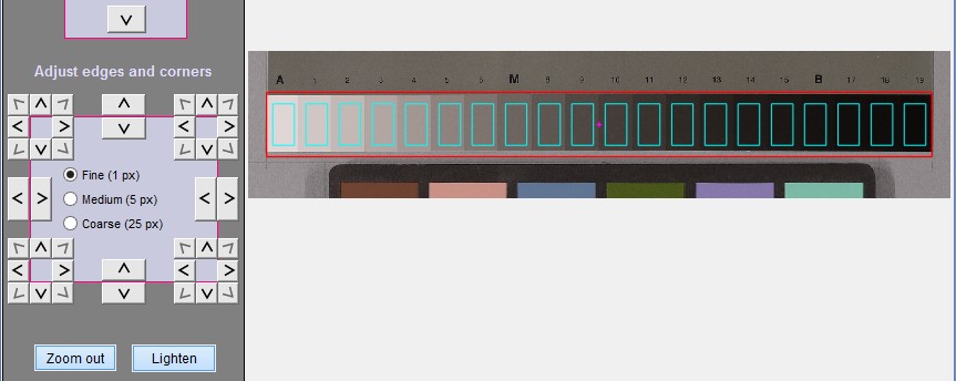 Fine ROI selection (dialog box detail) lets you preview region locations: Details here.
Incident lux (for ISO Sensitivity calculations) When a positive value of incident light level (not blank or zero) in lux is entered in this box, ISO sensitivity is calculated and displayed in the Stepchart noise detail figure. More details are on the ISO Sensitivity and Exposure Index page. Also required if Lux is selected for the X-axis scale (figs 2-4).
Aperture and Exposure must be entered for the x-axis of Figures 2-4 to be displayed in units of Lux. They are normally obtained from EXIF datan if available, but they may be entered manually if needed.
Saturation level The maximum pixel level for the input image, corresponding to saturation level, used for normalizing image data for certain calculations. Selections:
| Standard file: 255 | The saturation level is automatically set based on the data type and container size of the image data. This is the default setting. The image file is assumed to have standard bit depth (e.g., 8, 16, or 32 -bit data) and standard saturation level. For example, for standard 8-bit image data, saturation level will be set to 255. For a 16-bit image, saturation level will be set to 65535, and for a 32-bit image, saturation level will be set to 4294967295. |
| ITU-R Rec. 601 (BT.601): 235 | The saturation level is set to 235. |
| Maximum detected patch level | The saturation level is set to the maximum detected value from the patch regions in the image. Can be useful if the image data is of nonstandard bit depth (e.g., 12-bit data stored in a 16-bit container) or if there is a custom saturation level, so long as the image is exposed to saturate the brightest patches. |
| Manually-entered saturation level | The saturation level is set to the value entered by the user. Can be useful if the image data is of nonstandard bit depth or if there is a custom saturation level. For example, for an image that has 12-bit data stored in a 16-bit container, enter 4095 as the saturation level (2^12 – 1 = 4095). |
Scaling You can select the minimum value of the x-axis for figures 2 and 3. This setting defaults to Auto. Setting it manually allows several successive runs to be scaled identically, which can clarify comparisons between different cameras.
Results (Fig. 1), Lower plot: Pixel noise Three noise displays are available for the lower-left plot in first figure.
| Noise (%) normalized to image density range = 1.5 (not recommended) |
Values 0-1. (This setting is an approximation to scene-referenced noise, and is no longer recommended.) |
| Noise (%) normalized to 255 pixels (max of 100) |
Values 0-1. Noise will be worse for higher contrast cameras (affected by the gamma encoding) |
| Noise in pixels (maximum of 255) | Values 0-255. |
Noise Detail (Fig. 2), Middle plot: f-stop noise or SNR Two types of display are available for the middle-left plot of the second figure. The effects of gradual illumination nonuniformities have been removed from the results.
| f-stop noise | Scene-referenced noise, based on f-stops (factors of 2 in exposure or illumination) |
| SNR (based on f-stops) | Scene-references Signal-to-Noise Ratio, based on f-stops. Note that there are many ways of defining SNR. Most are image (or pixel)-referenced. Results are different from S/N in the lower plot (which is more standard). |
The scaling (minimum and maximum values) can be set in the dropdown menus to the right of the radio buttons. Most of the time these should be left at Auto. The values are inverted when the display is toggled between F-stop noise and SNR. For example, the minimum value of the x-axis in both Figures 2 and 3 can be set between -4 and -1.5.
Noise Detail (Fig. 2), Lower plot: Pixel noise or SNR Five types of display are available for the lower-left plot of the second figure. The first three are the same as the lower plot of Fig. 1. The effects of gradual illumination nonuniformities have been removed from the noise results. All displays are derived from Noise in pixels (the third selection below). In the notation below Ni is RMS noise and Si is signal (pixel) level for patch i.
| Noise (%) normalized to image density range = 1.5 | 100% * (Noise in pixels) divided by (the difference in pixel levels between light and dark patches that have a density difference of 1.5). This difference is close to the 1.45 White-Black difference in the ColorChecker. Useful because it references the noise to the scene: noise performance is not affected by camera contrast. |
| Noise (%) normalized to 255 pixels (max of 100) | 100% * (Noise in pixels) / 255 = Ni/2.55. Values 0-100. This noise measurement will be worse for higher contrast cameras. (It is affected by the gamma encoding.) |
| Noise in pixels (maximum of 255) | Noise in pixels ( Ni ). Values 0-255. |
| Pixel S/N (Signal in patch/RMS noise) dimensionless | Noise in pixels ( Ni ). Values 0-255. |
| Pixel SNR (dB) (20*log10(S/N)) | 20 Log10(signal/noise) for each patch (where signal = pixel level). Units of dB (decibels). Doubling S/N increased dB measurement by 6.02. |
| For this selection, SNR_BW is also displayed. SNR_BW is an average SNR based on White-Black patch levels (density difference = 1.5), close to the W-B difference in the ColorChecker. It’s designed to be relatively independent of the chart type and system contrast (gamma). SNR_BW = 20 log10((SWHITE–SBLACK )/Nmid ), where Nmid is the noise in a middle gray patch (closest to nominal chart density = 0.7). |
X-axis scale (Figs 2-4) and Dynamic Range units (Fig. 2) Several choices are available, including Density units, EV, Lux (if incident Lux, Aperture, and Exposure are available) and dB (decibels: 20*density units). DR units may or may not be the same as the scale units. The old default was scale in Log exposure and Dynamic Range in EV (the first selection). Note: 1 Density unit = 3.322 EV = 20 dB; 1 EV = 6.02 dB. Selections:
Log exposure (-target density) for x-axis. Dynamic Range in EV.
Lux (incident Lux / 10^density) for x-axis. Dynamic Range in EV.
Exposure in dB (-20*Target density) for x-axis. Dynamic range in dB.
Log exposure for x-axis. Dynamic Range in Density units.
F-stops (EV) for x-axis. Dynamic Range in EV (F-stops).
The Plot box on the right lets you select figures to display. Two files must be read in to obtain the Temporal noise plot.
When all settings have been made, click to continue.
Results
The example was photographed with the Canon EOS-10D at ISO 100 and converted from RAW format using Capture One with default settings (no curves applied).
The results include tonal response and noise. Colorcheck produces a similar result, but with less tonal detail. Three figures are produced for color images; two for B&W.
First Figure: Stepchart results
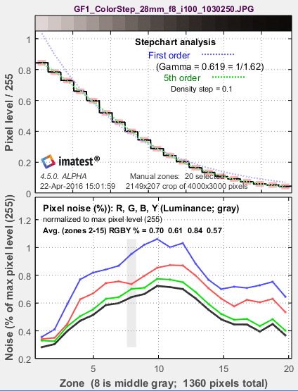
The upper plot shows the mean normalized pixel level of the grayscale patches (black curve) and first and second order density fits (dashed blue and green curves). The horizontal axis is the zone (patch number; proportional to the distance along the target for linear charts). A portion of the patches themselves are shown just above the plot. The equations for the density fits are given in the Algorithm section, below. The second order fit typically closely matches the patches. For automatic zone detection, the differentiated and smoothed steps used to find the boundaries between zones are displayed as light cyan spikes (not shown).
The lower plot shows the RMS noise for each patch: R, G, B, and Y (luminance) in units selected in the Settings Window (above). For this display, noise measured in pixels can be calculated by multiplying the percentage noise by 255.
Noise can be normalized to 255 pixels, expressed in pixels (maximum of 255), or normalized to the pixel difference corresponding to a target density range of 1.5 (the same as the white – black patches on the X-Rite ColorChecker). Options are described above.
Noise is largest in the dark areas because of gamma encoding: In the conversion from the sensor’s linear output to the color space (sRGB, here) intended for viewing at gamma = 2.2, the dark areas are amplified more than the light areas and the noise is boosted as well.
See Noise in photographic images for a detailed explanation of noise: its appearance and measurement.
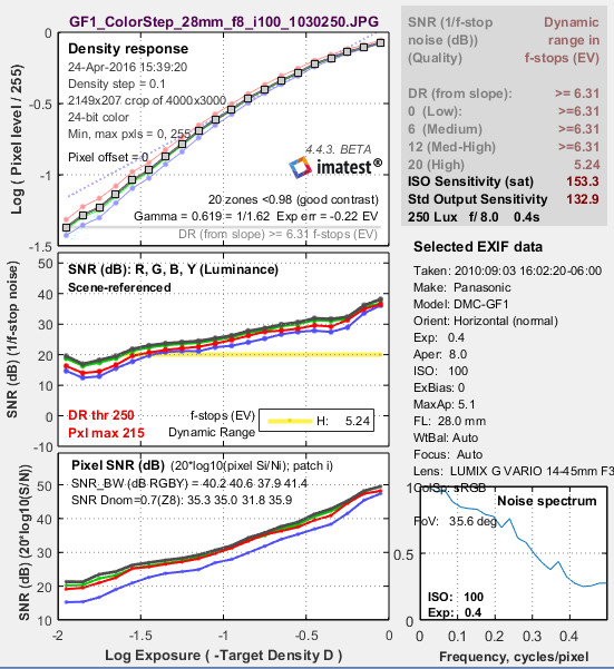
Second figure: Stepchart noise detail
The second figure (Noise detail) contains some of the most important results:
- the tonal response curve (displayed on a log scale, similar to film response curves),
- noise expressed as either a fraction of an f-stop (or EV or zone), or Scene-referenced Signal-to-Noise Ratio (SNR = S/N = 1/f-stop noise),
- noise or SNR (signal-to-noise ratio), based on pixel levels, expressed in one of several ways, and
- dynamic range (only reliable for transmission step charts because reflective charts have a smaller tonal range than most cameras).
The horizontal axis for the plots below is Log Exposure, which equals (minus) the nominal target density (log10(light(out)/light(in) ) = 0.05 – 1.95 for the 20-step Q-13/Q-14 charts). This axis is reversed from Figure 1. The axis can also be set to f-stops (EV; factors of 2; -3.32*density) or decibels (dB; -20*density)
|
The upper left plot shows the density (tonal) response (gray squares), as well as the first and second order fits (dashed blue and green lines). Density (logarithmic) plots correspond to the workings of the human eye. They resembles a traditional film density response curves. Dynamic range is grayed out because the reflective Q-13 target has too small a density range to measure a camera’s total dynamic range. See Dynamic range, below. This curve is closely related to the Opto-Electronic Conversion Function (OECF), which is a linear curve of exposure vs. pixel level. Exposure error (Exp err) is described here.
|
The upper right box contains dynamic range results: the slope-based dynamic range (Imatest 4.5+) and the range for several quality levels, based on luminance (Y) noise. Details below. It is shown in gray when a reflective target is selected. |
|
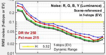
The middle left plot shows the scene-referenced Signal-to-Noise Ratio (SNRscene) in dB (the inverse of the noise in f-stops (or EV), shown below, which is the noise scaled to (divided by) the difference in pixel levels between f-stops). SNR tends to decrease (noise increases) as brightness decreases. The logarithmic vertical axis displays dark area noise levels clearly. Dynamic range information is displayed when the range for a specific quality level (defined by maximum f-stop noise or minimum SNR) is within the range of the plot. It is omitted if noise or scene-referenced SNR is better than the specified level for all patches: it is not reported for quality levels lower than H in the above plot because SNR never drops below 12dB (f-stop noise < 0.25): the M-H level).
f-stop (scene-referenced) noise (1/SNRscene ) can bedisplayed in the middle-left plot in place of SNRscene.
|
The x-axis (log exposure) is reversed in direction from Figure 1, |
|
The lower left plot shows pixel noise or SNR displayed in one of several different ways. The above-right illustration shows pixel SNR (dB) = 20 log10(Si/Ni), where Si is the signal (mean pixel level) of patch i and Ni is the noise (standard deviation of the pixel level, with slow variations removed) of patch i. The plot below is the lower left plot set for pixel noise normalized to 100%.
|
The middle right region shows selected EXIF data (metadata). The lower right plot shows the noise spectrum for a middle gray region. Demosaicing by itself causes the spectrum to drop to about 0.5 at the Nyquist frequency (0.5 cycles/pixel). Digital camera images with strong noise reduction will have more rapid falloff. SNR_BW is an average SNR for signal S based on white-black patch levels (density difference = 1.5), which is the Black-White density difference for the Colorchecker. It’s designed to be relatively independent of the chart type and system contrast (gamma). |
 Second figure: noise detail, ISO 100
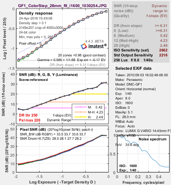 Second figure: noise detail, ISO 1600 Second figure: noise detail, ISO 1600 |
Here are the results for ISO 1600. Tonal response is similar to ISO 100, but SNR is significantly decreased (noise is increased). The noise is highly visible, but the image is still useful for many purposes. It might not be suitable for fine portraits, but it would be acceptable when a grainy “Tri-X” or “available light” look is desired. The middle-left plot displays dynamic range for several quality levels, specified by the minimum SNRscene (maximum noise) within the range. The dynamic range for low quality (L; blue) has a minimum SNRscene of 0dB (1:1; a maximum noise of 1 f-stop); the dynamic range for high quality (H; yellow) has a minimum SNRscene of 20dB (10:1; a maximum noise of 0.1 f-stop). |
Third Figure: Density and contrast response
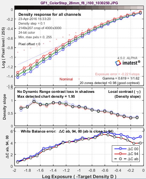
The upper plot shows the density response (small circles) of the luminance (Y), red, green, and blue channels, as well as the first and second order fits (dotted and dashed gray lines). It resembles a set of traditional film density response curves. The R, G, and B curves are not displayed in Imatest Studio.
For reflection step charts only, the nominal exposure is shown as pink dots (•), and the exposure error in f-stops is displayed. Exposure error is less critical than for Colorcheck, where it strongly affects the a*b* color values: that’s why it isn’t displayed in the other figures. The equation for nominal exposure is similar to equation that calculates the grayscale pixel levels of the ColorChecker:
pixel level = 255 * (10–density/1.01)(1/2.2)
The middle plot shows the slope of the density curve, which can also be regarded as the local contrast or gamma. This curve is the derivative of the density, d(Density) / d(Log Exposure).
The lower plot is the color error, measured as ΔCab (geometrical distance in the CIELAB a*b* plane), ΔC94 , and ΔC2000. They are quite close because chroma tends to be quite low for grayscale patches.
Lens flare (stray light that bounces between lens elements and off the barrel) can be measured by photographing a reflective step chart (a Q-13 or Q-14) against dark and white backgrounds. When flare light is present (white background) it will reduce the slope of the density response in dark regions of the step chart (on the left of the plot). This curve makes it easy to measure the decrease in the slope.
Fourth figure: Temporal noise
Temporal (time-varying) noise is the random difference between otherwise identical images. It is measured as the noise (standard deviation) of the difference two identical test chart images divided by the square root of 2 (1.414).
Ntemporal = Noise(Image1-Image2) / 1.414
Subtracting two images removes fixed pattern noise. The square root of 2 is needed because noise powers add, even though image pixels are subtracted. Dividing by the square root of 2 scales temporal noise to be the same as noise measured in an individual image.
To measure temporal noise, select two images for analysis. In the dialog box shown on the right, select Read two files for measuring temporal noise. The analysis proceeds normally (for the first file), but a fourth figure, displayed if 4. Temporal noise is checked in the input dialog box Plot area, contains the temporal noise analysis. This figure is intended to be self-contained, hence repeats some features of previous plots.
Temporal noise display
- The upper-left plot displays the density response, similar to the upper-left plot of Figure 2.
- The lower-left plot (RMS noise (f-stops)) displays scene-referenced noise or SNR using the same scale as the middle-left plot of Figure 2. In these plots, noise (or SNR) for a single image is shown as a pale curve.
- The upper-right plot (Pixel SNR (dB)) displays noise or SNR using the same scale as the lower-left plot of Figure 2.
- The lower-right plot (Noise in pixels) displays pixel noise scaled the same as the lower plot of Figure 1 (for the vertical axis; the x-axis is different).
Saving the results
|
When the Stepchart calculations are complete, the Save Stepchart Results? dialog box appears. It allows you to select figures to save and choose where to save them. The default is subdirectory Results in the data file directory. You can change to another existing directory, but new results directories must be created outside of Imatest— using a utility such as Windows Explorer. (This is a limitation of this version of Matlab.) The selections are saved between runs. You can examine the output figures before you check or uncheck the boxes. Figures, CSV, and XML data are saved in files whose names consist of a root file name with a suffix and extension. The root file name defaults to the image file name, but can be changed using the Results root file name box. Be sure to press enter. Checking Close figures after save is recommended for preventing a buildup of figures (which slows down most systems) in batch runs. After you click on or , the Imatest main window reappears.
|
 Save dialog box |
Dynamic range of cameras and scanners
| For a more comprehensive and up-to-date explanation of Dynamic Range, we recommend the Dynamic Range page. |
Imatest can calculate Dynamic Range in several modules using several types of test chart.
| Dynamic range from a single transmissive chart image. | Stepchart, Color/Tone Interactive, Mutitest | A transmissive chart is such as the Imatest 36-patch Dynamic Range or HDR chart is required because reflective charts do not have sufficient tonal range. |
| Dynamic range from multiple (differently exposed) images | Dynamic Range module | Uses CSV output of Stepchart of Color/Tone Auto for several differently exposed images. Usually used with reflective charts, but transmissive charts may also be used. No longer recommended because it fails to account for the effects of flare light. |
| ISO 15739 Dynamic Range from patch with density ≈ 2 | Color/Tone Interactive, Color/Tone Auto, eSFR ISO | Extrapolates Dynamic Range from a single patch with density ≈ 2. |
| Raw sensor Dynamic Range | Color/Tone Interactive, Color/Tone Auto | Fits raw data to an equation from the EMVA 1288 standard, then extrapolates to find DR. The test chart does not have to have as large a tonal range as the DR, but transmissive charts with tonal range ≥ 3 are recommended. |
Dynamic Range definitions
Dynamic Range (DR) is the range of scene brightness (tones) over which a camera responds with good contrast and/or a good Signal-to-Noise Ratio (SNR).
Imatest Dynamic range can be defined in two ways.
| Quality-based | the range of tones over which the scene-referenced SNR (SNRscene) is greater than a specified minimum amount (the f-stop noise remains below a specified maximum value). The higher the SNRscene (the lower the noise) in a region, the better the image quality. SNR tends to be worst in the darkest regions. Imatest calculates the dynamic range for four SNR levels, SNR. Recommended in most cases. | SNR = 10 (20dB; high quality) SNR = 4 (12dB medium-high quality) SNR = 2 (6dB; medium quality) SNR = 1 (0dB; low quality) |
| Slope-based (introduced in Imatest 4.4) |
The range of tones where slope of the density curve is greater than 7.5% of the maximum slope (on the dark side) and less than 98% of the saturation level (on the light side). This has to be done with care since noise and irregular density steps in the original data affects patch levels, and hence slope measurement. Test chart density is interpolated to have 101 evenly-spaced points, then the log pixel level for these points is found using the Matlab interp1 function. The curve is smoothed using a rectangular kernel 7 points wide (approximately 1/13 of the total range). This algorithm gives stable, robust results, much better than earlier (pre-4.4) Patch range and detected DR measurements. This method is not typically used for pictorial imaging because noise can be severe in the darkest regions. |
|
Dynamic range can be expressed in any of the following units.
- f-stops, or equivalently, zones or EV (factors of two; log2 units),
- density (log10) units, where one density unit = 3.322 f-stops, or
- decibels (dB), where 1 density unit = 20dB; 1 f-stop = 6.02dB.
The dynamic range corresponding SNRscene = 1 (0dB; 1 f-stop of noise) corresponds to the intent of the ISO 15739 Dynamic range definition in section 6.3 of the ISO noise measurement standard: ISO 15739: Photography — Electronic still-picture imaging — Noise measurements. The Imatest measurement differs in several details from ISO 15739; hence the results are not identical. Imatest may well produce more accurate results because it measures DR directly from a transmission chart, rather than extrapolating results for a reflective chart with maximum density = 2.0.
The most straightforward way to measure a camera’s (or scanner’s) dynamic range is with a transmission step chart illuminated from behind by a lightbox. Reflection step charts such as the Kodak/Tiffen Q-13 or Q-14 are inadequate because their density range of around 1.9 is equivalent to 1.9 * 3.32 = 6.3 f-stops, well below that of digital cameras (though several different exposures can be combined in the Dynamic Range postprocessor for Stepchart and Color/Tone Auto).
Transmission step chart
The table below lists several transmission step charts, all of which have a density range of at least 3 (10 f-stops). Kodak Photographic Step Tablets can be purchased calibrated or uncalibrated. Uncalibrated is usually sufficient. The Stouffer charts are attractively priced.
| Product | Steps | Density increment | Dmax | Size |
| Imatest 36-patch Dynamic Range test chart (recommended) |
36 | ~0.10 (1/3 f-stop); Reference file included |
3.4 | 8×10″ |
| Imatest 36-patch High Dynamic Range test chart (also recommended) |
36 | ~0.10 – 0.30 (1/3 – 1 f-stop); Reference file required |
>6 | 8×10″ |
| Kodak Photographic Step Tablet No. 2 or 3 | 21 | 0.15 (1/2 f-stop) Linear pattern | 3.05 | 1x5.5″ (#2) larger (#3) |
| Stouffer Transmission Step Wedge T2115 | 21 | 0.15 (1/2 f-stop) Linear pattern | 3.05 | 0.5x5″ |
| Stouffer Transmission Step Wedge T3110 | 31 | 0.10 (1/3 f-stop) Linear pattern | 3.05 | 3/4x8″ |
| Stouffer Transmission Step Wedge T4110 | 41 | 0.10 (1/3 f-stop) Linear pattern | 4.05 | 1x9″ |
| Danes-Picta TS28D (on their Digital Imaging page) |
28 | 0.15 (1/2 f-stop) Linear pattern | 4.2 | 10x230 mm (0.4x9″) |
| DSC Labs 72-dB 13-step Greyscale | 13 | 0.30 ( 1 f-stop) Linear pattern | 3.7 | (large) |
| Esser Test Charts TE 241 | 20 | from table; large in dark regions Circular pattern of squares |
4.1 | (large) |

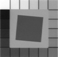
The Stouffer T4110 (13.3 f-stops range), Danes-Picta TS28D (13.6 f-stops range), or TE 241 (13.6 f-stops range) are often used for Digital SLRs, which can have dynamic ranges over 10 f-stops. The Stouffer T4110 (shown on the right) is inexpensive and has Dmax = 4.0, but is difficult to frame, difficult to expose properly with auto-exposure cameras, and susceptible to light falloff due to its linear arrangement.
The Imatest 36-patch Dynamic Range test chart, with density steps of approximately 0.1 from base density to base+3.4 (an 11.3 f-stop range) or the 36-pach High Dynamic Range (HDR) test chart, with density steps from 0.1 to 0.3 and a maximum density of at least base+6 (20 f-stops), are strongly recommended. A nearly circular patch arrangement ensures that vignetting has minimal effect on results. A CSV or CGATS reference file with actual densities (required with the HDR chart) is supplied. the chart has an active area of 7.75×9.25 inches on 8×10 inch film.
It also contains slanted edges in the center and corners with 4:1 contrast for measuring MTF. The edges have an MTF50 >= 16 cycles/mm, which is about 3 times better than the best inkjet charts. Registration marks make the regions easy to select, and fully automated region detection is available in Imatest 4.0+. A neutral gray background helps ensure that the chart will be well-exposed in auto exposure cameras (compared to charts with black backgrounds, which are sometimes strongly overexposed).
The standard 36-patch Dynamic Range chart can be used with the Dynamic Range postprocessor to measure dynamic ranges larger than 11 f-stops if several manual exposures are available. Dmax = 3.4 is sufficient for camera phones and digital cameras with small pixel sizes, but high-end DSLRs and HDR security and automotive cameras generally have higher dynamic ranges, which makes them well suited for measurements with either Dynamic Range or the HDR chart (which never requires the Dynamic Range postprocessor).
 Imatest 36-patch Dynamic Range chart Imatest 36-patch Dynamic Range charton 8×10 film. Dmax ≈ 3.4. |
 Imatest 36-patch High Dynamic Range chart Imatest 36-patch High Dynamic Range charton 8×10 film. Dmax > 6.0. |
This chart is produced with a high-precision LVT film recording process for the best possible density range, low noise, and fine detail.
Lightbox
 You’ll need a lightbox that can evenly illuminate the transmission step chart. 9×12 inches is large enough in most cases. Avoid thin or “mini” models, which may not have even enough illumination. Fluorescent light boxes should have high frequency ballasts to eliminate flicker. The GLE-10 and GLE-16E, available in the Imatest store are recommended. LED light boxes (for example, the Artograph 12×9 inch model) are nice because they’re inexpensive, flicker-free (DC power supplies) and easy to dim (if you have a current-limited DC power supply), but they are not reliable for color measurements.
Lightboxes available from the Imatest Store are compared in the Lightbox Comparison Guide.
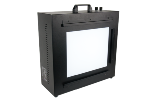
The best available lightbox is the Imatest LED Lightbox (shown on the right), available from the Imatest store. It has several advantages over the lightboxes mentioned in the previous paragraph.
- Much more uniform illumination: up to 95% uniformity.
- High quality spectral response. The standard version allows you to choose from 3100K, 4100K, 5100K, 5500K, 6500K and NIR color temperatures (850nm or 940nm) with a Color Rendering Index (CRI) of 97.
- Intensity is adjustable via a hardware knob, Bluetooth, or USB from as low as 1 lux and up to 100,000 lux: a range of over 300:1, making it suitable for measurements from near-daylight to extremely dim light.
| INCIDENT LIGHT MEASUREMENT
Reflective charts: Incident light measurement is relatively straightforward. Place an incident illumination meter with a flat diffuser (such as the inexpensive BK615) just in front of the chart, pointed towards the camera, making sure not to block any of the illumination. Use the lux measurement directly. Transmissive charts: These are not so straightforward: the lux measurement cannot be used directly. You will need to measure a clear (white) area of the chart (not the lightbox itself). For meters like the BK 625, where you can switch the orientation of the sensor, set it to point towards the light source (on the opposite side from the display). Measure the illumination in a white area of the chart. For the 36-patch Dynamic Range chart, use the lightest grayscale patch. You need to make an adjustment because the input to Imatest is designed for reflective charts, where white areas reflect about 90% of the incident light. To compensate for this, use Lux (input to Imatest) = Lux (measured) * 1.11. Useful equation: If your meter reads in EV (Exposure Value): Lux = 2.5 * 2EV @ ISO 100 |
Measuring dynamic range
- Place the chart on the lightbox— or any source of uniform diffuse light. Be sure to block direct light from the lightbox outside of the chart: Stray light can reduce the measured dynamic range; it should be avoided.
- Photograph the chart in a darkened room. No stray light should reach the front of the target; it will distort the results. The surroundings of the chart should be kept as dark as possible to minimize flare light.
- Use your camera’s histogram to determine the minimum exposure that saturates the lightest region of the chart. Overexposure (or underexposure) reduces the number of useful zones. The lightest region should have a relative pixel level of at least 0.98 (pixel level 250 or 255); otherwise the full dynamic range of the camera will not be detected. If the lightest zone is below this level, and a transmission chart is selected, a Dynamic range warning is issued.
-
For flatbed scanners with transparency units (TPUs, i.e., light sources for transparencies), you can simply lay the step chart down on the glass. Stray light shouldn’t be an issue, though there is no harm in keeping it to a minimum. 35mm film scanners may be difficult to test since most can only scan 36mm segments. (Most transmission targets are longer.) For scanners specified as having Dmax greater than 3, the charts of choice are the Stouffer Transmission Step Wedge T4110 or Danes-Picta TS28D, which are too large to be tested easily with 35mm film scanners.
- Follow the remainder of instructions in Photographing the chart and running Stepchart, above. Be sure to select the correct chart type from the Stepchart input dialog box (right).
Interpreting Dynamic Range
The dynamic range is the difference in scene brightness ( (–) chart density) between the zone where the pixel level is 98% of its maximum value (250 for 24-bit color, where the maximum is 255), estimated by interpolation, and the darkest zone that meets the measurement criterion (minimum SNRscene or density response slope). The repeatability of this measurement is better than 0.5 f-stop.
| Dynamic Range criterion | Limits | Comments |
| Quality (minimum scene-referenced SNR) | 10, 4, 2, or 1 (ratio) 10, 12, 6, or 0 (dB) |
The recommended measurement in most cases. Image sensor spec sheets typically define DR using a minimum SNR = 1 (0dB). |
| Slope (> fraction of maximum slope) | 0.05 of maximum | The slope measurement involves careful interpolation to make it robust. Darkest regions may be very noisy. |
Measured dynamic range is typically less than specified sensor dynamic range, primarily because of lens flare— stray light reflected between lens elements and off the barrel (on the interior of the lens). Different chart designs have different distributions of illumination, hence different amounts of lens flare. Some sensor manufacturers claim dynamic ranges over 120dB (for special High Dynamic Range (HDR) sensors), but no camera system (which include optics) can reach that level of performance. (100dB is about as good as we’ve heard of.)
Sensor dynamic range can be measured from absolutely raw images (no demosaicing or processing of any king) with Color/Tone Interactive or Color/Tone Auto using the technique described in Color/Tone Interactive/Color/Tone Auto/eSFR ISO Noise. It can also be measured with a sequence of flat field exposures (often involving calibrated neutral density filters). But these measurements should never be confused with a camera system measurements (especially for HDR systems) because each image has essentially zero dynamic range.
Here is a result for the Panasonic G3 (a Micro Four-Thirds camera with 3.75 micron pixel pitch) at ISO 160, converted from raw using dcraw with the following settings: Demosaicing: Normal RAW conversion (demosaiced), Output gamma: 2.2, White Balance: Camera, Output color space: 48-bit, Quality: Default.

Panasonic G3, ISO 160, Converted with dcraw.
The slope-based dynamic range is greater than 11 f-stops. The Dynamic Range at low quality level (scene-referenced SNR = 1 = 0dB) is 9.33 f-stops, decreasing to 5.68 f-stops at high quality level (SNR = 10 = 20dB). These results are unchanged for 24-bit raw conversion.
The shape of the response curve is a strong function of the conversion software settings. The plot below is for the same exposure, saved as a JPEG file inside the camera. Note that the transfer curve is quite different: it has a “shoulder” in the highlights, which improves pictorial quality by reducing the tendency of highlights to saturate (“burn out”). Dynamic Range is increased due to software noise reduction (absent in the dcraw conversion).

Panasonic G3, ISO 160, in-camera JPEG. Note the “shoulder.”
Dynamic range is improved due to software noise reduction.
Units for displaying Dynamic Range can be set in the X-axis scale (Figs 2-4) and Dynamic Range units (Fig. 2) dropdown menu. To convert dynamic range from f-stops into decibels (dB), the measurement normally given on sensor data sheets, multiply the dynamic range in f-stops by 6.02 (20 log10(2)). The dynamic range for low quality (f-stop noise = 1; SNR = 1) corresponds most closely to the number on the data sheets.
Summary .CSV and XML files
An optional .CSV (comma-separated variable) output file contains results for Stepchart. Its name is [root name]_summary.csv. An example is Canon_EOS10D_Q13_ISO400_crop_summary.csv.
The format is as follows:
| Module | SFR, SFR multi-ROI, Colorcheck, or Stepchart. |
| File | File name (title). |
| Run date | mm/dd/yyyy hh:mm of run. |
| (blank line) | |
| Tables | Tables are separated by blank lines. |
| The first table contains measured and ideal pixel levels and densities. | |
| The second table contains density = -log(exposure) and Y, R, G, and B densities (-log(pixel level/255)), assuming 8 bits/pixel. | |
| The third table contains the density differences (slopes) between the Y, R, G, and B patches. | |
| The fourth table contains two sets of Y, R, G, and B noise measurements for the the patches in the bottom two rows, described above. – Noise (%) normalized to image density range = 1.5 – f-stop noise |
|
| The fifth table contains S/N and SNR (dB) for the Y, R, G, and B channels, described above. | |
| (blank line) | |
| Additional data | The first entry is the name of the data; the second (and additional) entries contain the value. Names are generally self-explanatory (similar to the figures). |
| (blank line) | |
| EXIF data | Displayed if available. EXIF data is image file metadata that contains important camera, lens, and exposure settings. By default, Imatest uses a small program, jhead.exe, which works only with JPEG files, to read EXIF data. To read detailed EXIF data from all image file formats, we recommend downloading, installing, and selecting Phil Harvey’s ExifTool, as described here. |
This format is similar for all modules. Data is largely self-explanatory. Enhancements to .CSV files will be listed in the Change Log.
The optional XML output file contains results similar to the .CSV file. Its contents are largely self-explanatory. It is stored in [root name].xml. XML output will be used for extensions to Imatest, such as databases, to be written by Imatest and third parties. Contact us if you have questions or suggestions.
| Algorithm |
A simplified (first-order) equation for a capture device (camera or scanner) response is, normalized pixel level = (pixel level/255) = k1 exposuregamc Gamc is the gamma of the capture device. Monitors also have gamma = gamm defined by monitor luminance = (pixel level/255)gamm Both gammas affect the final image contrast, System gamma = gamc * gamm Gamc is typically around 0.5 = 1/2 for digital cameras. Gamm is 1.8 for Macintosh systems; gamm is 2.2 for Windows systems and several well known color spaces (sRGB, Adobe RGB 1998, etc.). Images tend to look best when system gamma is somewhat larger than 1.0, though this may not hold for contrasty scenes. For more on gamma, see Glossary, Using Imatest SFR, and Monitor calibration. log10(normalized pixel level) = log10( k1 exposuregamc) = k2 – gamc * density This is a nice first order equation with slope gamc, represented by the blue dashed curves in the figure. But it’s not very accurate. A second order equation works much better: log10(normalized pixel level) = k3 + k4 * density + k5 * density2 k3, k4, and k5 are found using second order regression and plotted in the green dashed curves. The second order fit works extremely well. |