Obtain and photograph chart – Lighting – Distance – Exposure – Tips – Links
Imatest Checkerboard performs highly automated measurements of sharpness (expressed as Spatial Frequency Response (SFR), Lateral Chromatic Aberration, and optical distortion from images of checkerboard patterns (with a recommended tilt angle of ~5-8 degrees for sharpness measurements).
The primary advantages of Checkerboard are:
- Compared to Imatest’s other automatically-detected sharpness modules: It is relatively insensitive to framing. You can zoom in or out as much as you like, as long as there are detectable corner features.
- Compared to the Distortion (legacy) module: It works with highly-distorted (fisheye lens) images. Calculations are more accurate, and it contains all results available in Distortion.
The disadvantages of Checkerboard are:
- Significant optical aberrations, blooming, or blemishes may cause the corner points to be missed, resulting in a loss of analysis area. (Distortion has similar issues.)
- Color and tonal response, available with SFRplus and eSFR ISO, are not available.
- Chart detection is slower than SFRplus and eSFR ISO, especially for large or strongly distorted images. (This is a Matlab issue that might be fixed in the future.)
- Some display images with visible pixel patterns can cause the detection algorithm to go into a (near) infinite loop.
Details of the regions to be analyzed are based on user-entered criteria (similar to SFRplus, eSFR ISO, or SFRreg, which it closely resembles).
Sharpness is derived from light/dark edges in the checkerboard pattern (which should be tilted), as described in Sharpness: What is it and how is it measured?
Checkerboard operates in two modes.
- Interactive/setup mode (run by pressing Rescharts in the Imatest main window, then selecting 11. Checkerboard, or by run by pressing the Interactive/Postprocessors dropdown menu, then selecting Checkerboard setup), allows you to select settings and interactively examine results in detail. Saved settings are used for Auto Mode.
- Auto mode (run by pressing the Fixed modules dropdown menu in the Imatest main window, then selecting Checkerboard— a button may be added later), runs automatically with no additional user input. ROIs are located automatically based on settings saved from the interactive/setup mode. This allows images of different sizes and framing to be analyzed with no change of settings. Auto mode works with large batches of files, and is especially useful for automated testing, where framing may vary from image to image.
This document introduces Checkerboard and explains how to obtain and photograph the chart. Part 2 shows how to run eSFR ISO interactively inside Rescharts and how to save settings for automated runs. Part 3 and Part 4 illustrates the results for slanted-edge and other measurements, respectively.
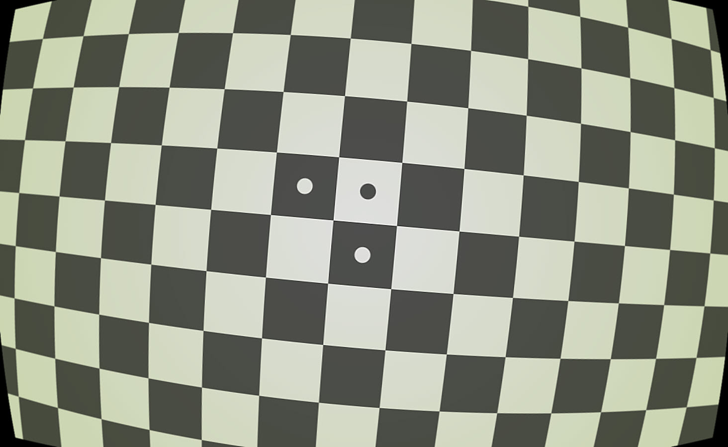 Checkerboard image (simulated): Click on image to download for analysis.
| Options | Notes | |
|---|---|---|
| Media | Inkjet (reflective), LVT film (transmissive) |
Inkjet (reflective) is usually the most practical choice. |
| Contrast |
4:1, 10:1, 45:1, 100:1 |
4:1 contrast is specified in the ISO 12233:2014 standard. |
| Surface | Matte or glossy film |
Matte surfaces are recommended for wide angle lenses or difficult lighting situations. The glossy high precision charts are sharper, but more susceptible to glare (specular reflections), especially with wide angle lenses. |
| Slanted-edge algorithm The algorithms for calculating MTF/SFR were adapted from a Matlab program, sfrmat, written by Peter Burns ( |
Example: highly distorted image with lines and arrows
The relationship between the original and corrected image can be displayed (in Checkerboard-only) when Display arrows & lines is selected in the Display options area of the More settings window. The lines in the original image (below, left) give a good visual indication of how well the calculated coefficients correct the distortion.
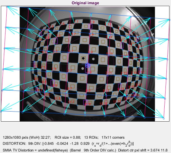 Original image Original image |
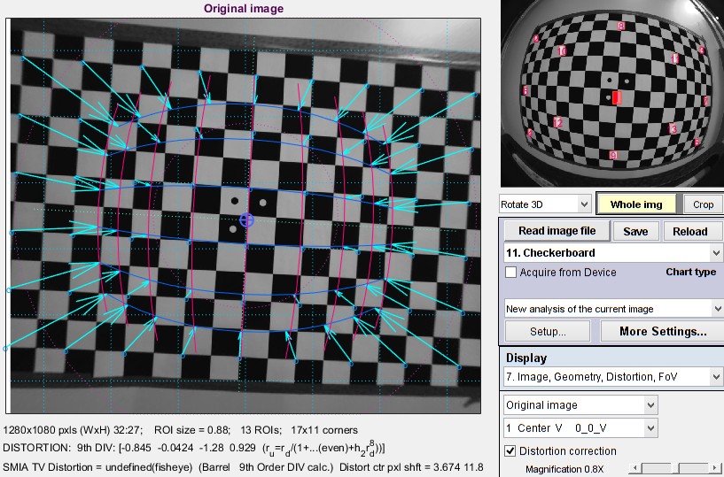 Corrected image Corrected image |
The magnification for the corrected image can be adjusted a slider on the lower-left of the Rescharts display area.
Obtain the chart
Checkerboard charts are available from the Imatest store on a variety of reflective and transmissive medium. Although we recommend that you purchase the charts, they can be printed on photographic-quality inkjet printers if you have high quality materials, skill, and a knowledge of color management. Here are the settings.
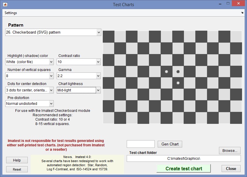 Typical settings for printing Checkerboard patterns
We recommend either 8 or 12 vertical squares. With fewer than 8, the distortion measurement may be less accurate. At least 5 rows of corners (1 less than the number of rows of squares) is required for a 5th order distortion calculation (needed for “mustache” or “wave” distortion). With more than 12, edges may become smaller than optimum for MTF measurements and calculations become slower. There is no practical advantage to more than 12 vertical squares unless you plan to print very large and do a lot of zooming (in and out).
The chart center is defined by the corner between the two light circles inside dark squares. When the circles are present the shift of the chart center (from the image center) is reported.
Charts can be mounted on sheets of 1/2 inch (12.5 mm) thick foam board with a spray adhesive (such as 3MTM 77 or Photo Mount) or double-sided tape (such as 3MTM #568 Positionable Mounting Adhesive). 1/2 inch foam board stays flatter than standard 1/4 or 3/8 inch foam board. PVC board is also very promising: it may be more durable and it comes in a variety of sizes.
|
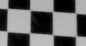
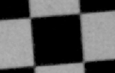
The Checkerboard algorithm searches for clean corners. We have seen cases where corners failed, for example, the patterns shown in the crops on the right. |
Photograph the chart
Framing the chart is not critical. Extreme flexibility is one of Checkerboard’s principal attributes.
The sides of the chart may extend beyond the image or be well within the image. The software is designed to accommodate a wide variety of framing and aspect ratios. If the sides of the chart are inside the image, you should try to minimize interfering patterns that could be mistaken for checkerboard corners. If possible, chart surroundings inside the image should be neutral gray, but this is not critical.
The Checkerboard Setup window image below shows the detected corners for an ideally-framed image. To measure regions near corners, the image should not be tilted too much. The image below is tilted 3 degrees, which is sufficient for slanted-edge measurements (except possibly for tiny images) and allows measurements reasonably close to the corners. It the tilt becomes much larger, measurements near the corners become more difficult. This is especially true for the Checkerboard (Matlab) detection algorithm (selected in the dropdown menu on the lower-left), which only detects complete rows and columns. The alternative detection algorithm (Checkerboard (Custom)) is much slower, but often picks up corners that aren’t in complete rows or columns.
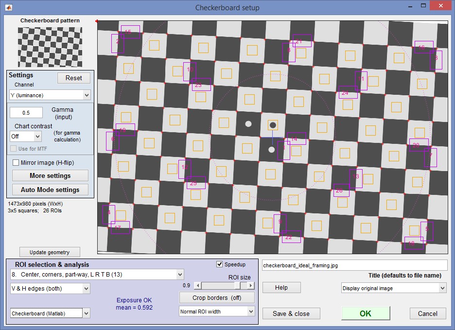 Checkerboard setup window for ideally-framed image
Tips:
- If possible, the chart should fill the image.
- If possible, the image should contain at least 6 and at most 16 vertical squares. Fewer than 6 will reduce the accuracy of distortion calculations; more than 16 slows the calculations and may cause regions (ROIs) to be smaller than optimum.
- For color and uniformity profile measurements, there must be at least 4 vertical light squares for vertical profiles (left/center/right), and at least 4 horizontal light squares for horizontal profiles (top/center/bottom). If there are fewer than 4 light horizontal/vertical squares in a region, the corresponding profiles will not be calculated.
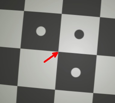
 Care should be taken to avoid interfering patterns outside the chart that could be mistaken for checkerboard corners.
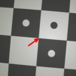
- If the chart contains the three dots that represent the image center, the corner between the three dots, indicated by the red arrow→ in the image on the right, should be as close as possible to the center of the image. It is used to calculate the x and y pixel shift.
- The environment should be close to middle gray (very roughly 18% reflectance) in order to obtain good exposures. (This may not be necessary if manual exposure control, i.e., exposure compensation, is available.)
- Avoid glare (shiny specular reflections). This easy for charts with a matte surface.
- Keep lighting reasonably even.
- For MTF measurements, the chart should be tilted around 2 to 7 degrees to avoid pure horizontal or vertical edges. Other orientations may work, but the region of analysis will be reduced. (The tilt is unnecessary for distortion-only measurements.)
- The image can be cropped to remove interfering features near the edges, using the Crop borders button in the Checkerboard setup window.
Lighting
The chart below shows ideal lighting, which may not be achievable for a set of registration mark patterns with fisheye lenses, but it’s good to be aware of. The goal is even, glare-free illumination and to avoid lights shining directly into the camera (which may be an issue with ultrawide fisheye lenses). Lighting angles between 25 and 45 degrees are ideal in most cases. At least two lights (one on each side) is recommended; four or six is better. Avoid lighting behind the camera, which can cause glare. Check for glare and lighting uniformity before you expose. Matte charts are recommended for wide angle lenses; it’s very difficult to control glare with semigloss surfaces.
Some recommended lighting configurations can be found in Building a Low-Cost Test Lab. The BK Precision 615 Light meter (Lux meter) is an outstanding low-cost instrument (about $100 USD) for measuring the intensity and uniformity of illumination.
 Simplified lighting diagram
Distance
|
A letter-sized (8.5×11 inch) chart printed on Premium Luster paper on the Epson 2200 (a high quality pigment-based inkjet photo printer) was analyzed for MTF using the 6.3 megapixel Canon EOS-10D. There was no change when the image field was at least 22 inches (56 cm) wide— twice the length of the chart. Performance fell off slowly for smaller fields.
Choose a camera-to-target distance that gives at least this image field width. The actual distance depends on the sensor size and the focal length of the lens. The minimum image field is illustrated on the right.
Cameras with more pixels, and hence higher potential resolution, should have a larger image field width, hence printed chart width.
Distance/field width guidelines for high quality inkjet charts
|
|
|||||||||||||||||||||||||||||||||||||||||||||||||
| Image field width (in inches) > 8.8 × sqrt(megapixels) Image field width (in cm) > 22 × sqrt(megapixels) — or —There should be no more than 140 sensor pixels per inch of target or 55 sensor pixels per centimeter of the target. — or —The distance to the target should be at least 40X the focal length of the lens for 6-10 megapixel digital SLRs.(25X is the absolute minimum for 6 megapixel DSLRs; 40X leaves some margin.) For compact digital cameras, which have much smaller sensors, the distance should be at least 100X the actual focal length: the field of view is about the same as an SLR with comparable pixel count. The recommended distance is described in more detail in Chart quality and distance, below. |
||||||||||||||||||||||||||||||||||||||||||||||||||
| There is some confusion about lens focal lengths in compact digital cameras. They are often given as the “35mm-equivalent,” which many photographers can relate to viewing angle. 35-105mm or 28-140mm are typical “35mm-equivalent” numbers, but they are not the true lens focal length, which is often omitted from the specs. What is given is the sensor size in 1/n inches, a confusing designation based on the outside diameter of long-obsolete vidicon tubes. It The table on the right relates the 1/ndesignation to the diagonal dimension of the sensor. True focal length = “35mm-equivalent” × (diagonal mm.) / 44.3 | ||||||||||||||||||||||||||||||||||||||||||||||||||
Exposure
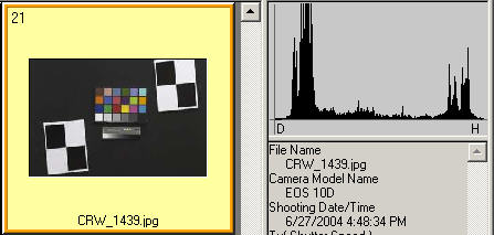
Good exposure is important for accurate Checkerboard results. Neither the dark nor the light regions of the chart should clip— have substantial areas that reach pixel levels 0 or 255. The best way to ensure proper exposure is to use the histogram in your digital camera. Blacks (the peaks on the left) should be above the minimum and whites (the peak(s) on the right) should be below the maximum.
The above image (taken from the Canon File Viewer Utility) is close to a perfect exposure. Some exposure compensation may be helpful.
|
Save the image as a RAW file or maximum quality JPEG. If you are using a RAW converter, convert to JPEG (maximum quality), TIFF (without LZW compression, which is not supported), or PNG. If you are using film, develop and scan it.
If the folder contains meaningless camera-generated file names such as IMG_3734.jpg, IMG_3735.jpg, etc., you can change them to meaningful names that include focal length, aperture, etc., with the Rename Files utility, which takes advantage of EXIF data stored in each file.
You are now ready to run Imatest Checkerboard.
Links
How to Read MTF Curves by H. H. Nasse of Carl Zeiss. Excellent, thorough introduction. 33 pages long; requires patience. Has a lot of detail on the MTF curves similar to the Lens-style MTF curve.
Understanding MTF from Luminous Landscape.com has a much shorter introduction.
Understanding image sharpness and MTF A multi-part series by the author of Imatest, mostly written prior to Imatest’s founding. Moderately technical.
Slanted-Edge MTF for Digital Camera and Scanner Analysis by Peter D. Burns (2000) (alternate source). An excellent introduction to the ISO 12233 slanted-edge measurement. Closely related: Diagnostics for Digital Capture using MTF by Don Williams and Peter D. Burns (2001), Applying and Extending ISO/TC42 Digital Camera Resolution Standards to Mobile Imaging Products by Don Williams and Peter D. Burns (2007) (Contains an image of an early version of the low-contrast slanted-edge test chart proposed for the revised ISO 12233 standard.)
Bob Atkins has an excellent introduction to MTF and SQF. SQF (subjective quality factor) is a measure of perceived print sharpness that incorporates the contrast sensitivity function (CSF) of the human eye. It will be added to Imatest Master in late October 2006.
How to Measure MTF and other Properties of Lenses by Optikos.