Create a synthetic test chart from several individual image files
Running – 1×N Linear charts – What to do with the Composite image – Settings
Photon Transfer Curves
Composite Chart can be used for two essential purposes.
- You may want to analyze colors in a microscopic image that has a field too small to capture an entire test chart (for example, a replica of the X-Rite Colorchecker, which is available in 35mm film size (24x36mm).
- You may want to combine several images to obtain tonal response and noise, following recommendations in certain ISO standards. This method is potentially useful for calculating Photon Transfer Curves.
To run Composite Chart, click the Utility dropdown menu (in the Imatest main window) and select Composite Chart. The following window opens.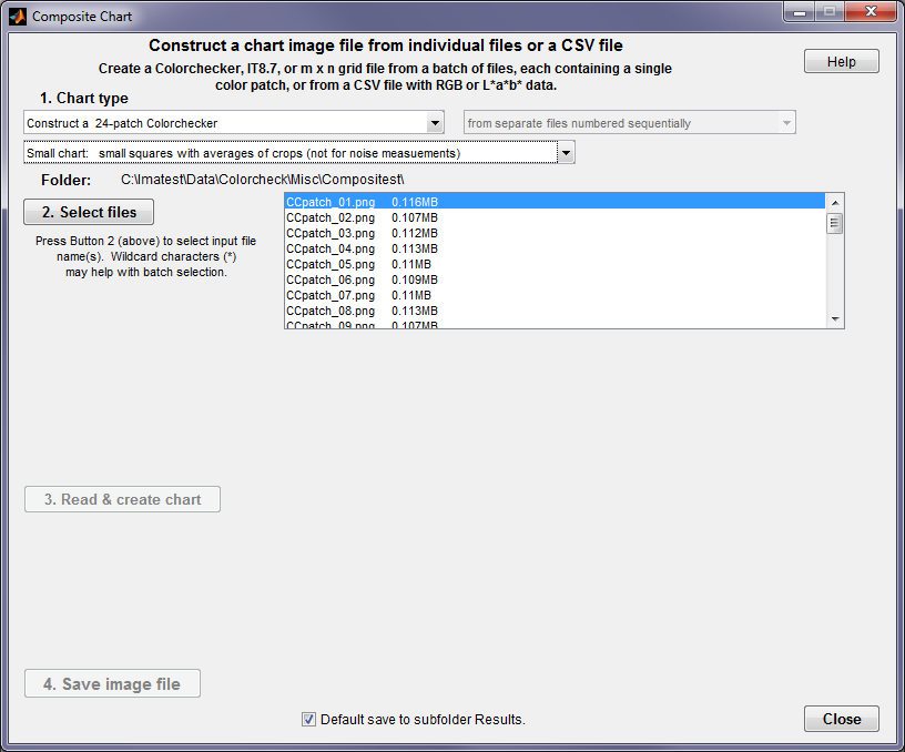
Composite Chart start window
First, select the chart type.
Options for chart types are
- Construct a 24-patch Colorchecker*.
- Construct an IT8.7 (rows A-L, columns 1-19: 228 patches). The first two were requested by a customer with a microscopic system where the field of view was too small to capture the entire chart. We don’t generally recommend the IT8.7 because has too many patches to be practical (it’s easy to make sequence errors).
- Construct a 1×N linear step chart*. This combines several images for certain ISO standard calculations. Any chart can be turned into a 1×N chart. This method may be used to create Photon Transfer Curves. You’ll need to save the L*a*b* or density reference file, as described below.
- Construct a 4×12 grid chart. This was a special customer request. We can easily add additional charts on request.
*These are the most popular charts: they are recommend unless you have a specific need for a different chart.
The second dropdown menu has two selections:
- Small chart: small squares with averages of crops (not for noise measurements) This is a good choice when colors and tones are to be analyzed (but not noise). patches are always square.
- Large chart: Use full crops (good for noise measurements, except for IT8.7) Patches maintain the aspect ratio of the crop (below, after images are read).
Second, press to choose the files to combine. The order will be based on a sort of the file name: we recommend that the names contain a numeric sequence. Use the usual techniques (shift-click, control-click; wildcard characters if needed) for selecting multiple files.
| Tip: To be ordered properly the input file names should contain a numeric sequence, where each number contains leading zeros. For example, file001.png, file002.png, … , filennn.png. |
Third, click .
You’ll be asked to crop the chart with the normal sequence of windows. If a crop selection has been saved, you’ll be asked if you want to repeat it. If not, you’ll be asked to enter a new crop. Here is a typical fine crop window.
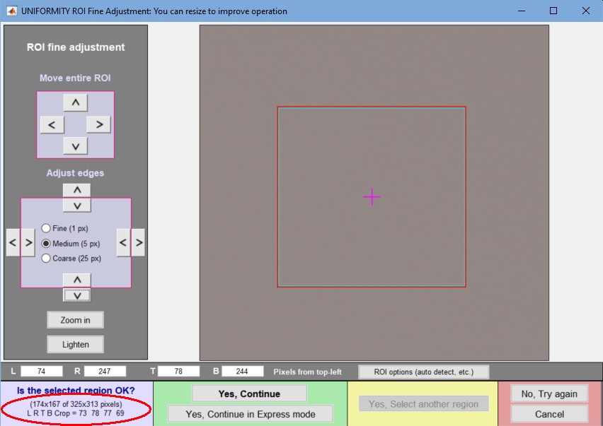 Fine adjustment window for cropping
The crop size is not critical, but if noise statistics are required the crop should be at least 100×100 pixels; between 200×200 and 400×400 is optimum. Very large crops (over 800×800) are unnecessary and may slow down the analysis of the results. Remember the final image will be larger than any of the crops, so for example, a 1×12 linear chart with a 400×400 pixel crop will have a total size of 400×4800 pixels.
Once the crop has been selected, the chart will be displayed.
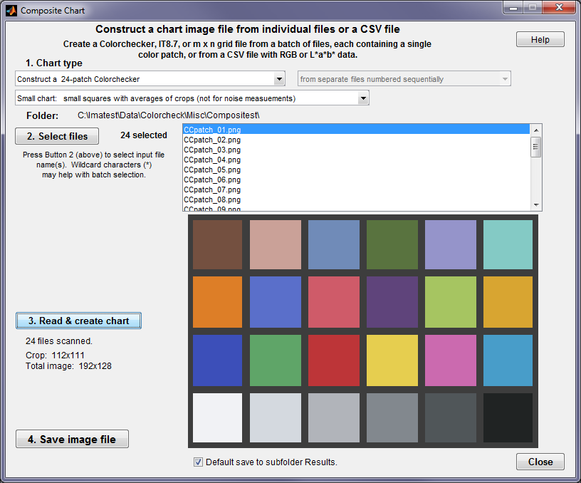 Composite chart window, showing the synthetic chart
If the chart image looks correct, click , and follow instructions.
Creating a 1×N (linear) chart from any chart
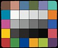
The basic procedure is straightforward. Select Construct a 1xN linear step chart from the Chart type dropdown menu. This is the result for the Colorchecker (selected because we happen to have the patches on hand). This is a good approach for other charts such as the 30-patch ColorGauge, shown below, which comes in small sizes, but may not be small enough for every application. Here is what the 1xn chart looks like for the 24-patch Colorchecker.
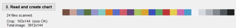 Composite chart: Linear Colorchecker
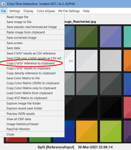
Copy the L*a*b* reference to the clipboard
The saved chart can be read into Color/Tone as a mxn chart with . The trick to making this work is to obtain a reference file. This can be done by running any sample of the original chart (e.g., the 4 row x 6 column Colorchecker or the 5×6 ColorGauge; it doesn’t have to be 1xN) the copying the L*a*b* reference file to the clipboard as shown on the right, pasting it into a text editor, then saving it for use as a reference file.
Here are the first 12 lines of the L*a*b* reference for the ColorGauge. Note that the order is row-major: start with the top row, left-to-right, then go to the second row, etc. Note that entries 8-11 are grayscale patches (very low a* and b*— in the second and third columns).
39.12 13.24 15.07
65.43 18.11 18.72
49.87 -4.34 -22.29
44.26 -13.8 22.85
55.56 9.82 -24.49
70.82 -33.43 -0.35
50.87 -27.17 -29.46
97.06 -0.4 1.13
92.02 -0.6 0.23
87.34 -0.75 0.21
82.14 -1.06 0.43
63.51 34.26 59.6
Open Color/Tone (Interactive or Auto). Before reading the image in Color/Tone Interactive, press Settings (dropdown menu), select ISO Speed, Noise, mxn chart …, then enter the number of rows and columns (1,24 for the linear Colorchecker) on the lower-right of the Color/Tone settings window.
What to do with the composite image
Most composite image files can be analyzed by Color/Tone Interactive or Color/tone Auto (formerly called Multicharts and Multitest). Legacy modules Colorcheck can also be used for the 24-patch Colorchecker and Stepchart can be used for grayscale charts, but we don’t recommend these for new work. The new modules have superior noise and dynamic range analysis, operate in both interactive and fixed (batch-capable) modes, and can be used for calculating Color Correction Matrices (CCMs).
We recommend running Color/Tone Interactive before running Auto — to verify that settings are correct. Once the settings look good in Interactive, it’s OK to run auto, which can analyze batches of images.
A reference file will usually be required. This file can have CSV or CGATS format. Typical files are csv density files, one density number per line or CSV CIELAB (L*a*b*) files, three numbers (L*, a*, b*) per line, separated by commas. Learn more about reference files here. For Photon Transfer Curves, you will need to create a CSV density file. For illumination L (with a maximum of Lmax),
\(density = -\log_{10}(L / L_{max})\)
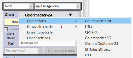
Settings
Before running Color/Tone Interactive, the chart must be selected in the Color/Tone Interactive window.
|
Selections for Colorchecker-24 and linear grayscale charts are shown.
|
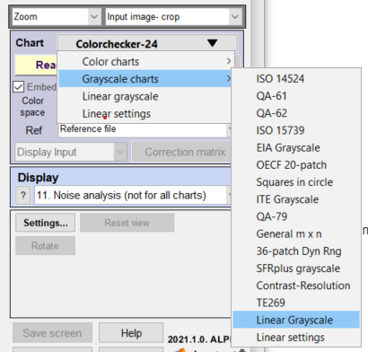 |
For linear grayscale charts (stepcharts), you will need to select the number of patches and the density reference (which can be steps of 0.1, 0.15, or 0.3 density units, or (more commonly) a density reference file. If you have light levels for each patch, recall that density is -log10(light level).
 Further instructions are in Using Color/Tone Interactive and Using Color/Tone Auto.
One more detail: some tiny charts are now available that were not available when Composite Chart was originally released. They may allow direct image capture without the need for Composite Chart. The most interesting among these are the ColorGauge, which comes in several sizes, and the Rezchecker.
| Chart Size | Height | Width | Thickness |
|---|---|---|---|
| Pico | 0.3750″ | 0.4375″ | 0.06″ |
| Nano | 0.6875″ | 0.8125″ | 0.06″ |
| Micro | 1.3750″ | 1.6250″ | 0.06″ |
Photon Transfer Curves
Imatest can be used to calculate Photon Transfer Curves following the method described in Characterizing Digital Cameras with the Photon Transfer Curve by David Gardner (of Summit Imaging at the time of publication).
- For characterizing image sensor performance, we recommend acquiring raw images and converting them to interchangeable files (TIFF, etc.) without demosaicing and with no additional image processing. Pixel offsets, if any, should be removed (this may involve converting commercial raw files to DNG). This approach is explained in Color/Tone & eSFR ISO noise measurements — Image sensor (RAW) noise and dynamic range.
-
Following the method in Data collection, for a set of calibrated light levels acquire 2 flat-field images for each light level. Name them so they can be processed in separate groups. The file name should be sortable. In most cases, this means including a numeric sequence with leading zeros: 001, 002, etc.
