including chroma, and visual noise as well as
several types of Dynamic Range calculation
|
Image Sensor Noise – measurement and modeling – using raw files for image sensor Dynamic Range and Simatest Using Color/Tone Interactive – Interactive analysis of color & grayscale test charts Using Color/Tone Auto – Fixed (batch-capable) analysis of color & grayscale test charts Dynamic Range – a general introduction with links to Imatest modules that calculate it. ISP/Camera Simulator (Simatest) – Image Signal Processing/Camera Simulator. Uses results from Color/Tone raw image analysis Noise in Photographic Images – a basic introduction Color Correction Matrix (CCM) Calculate a matrix (usually 3×3) for correcting image colors (often from RAW images) |
Introduction – Settings – Noise displays – Noise table – Imatest Dynamic Range (DR) –
Image sensor RAW noise and DR – Equations – Temporal noise – Chroma noise – Visual noise –
ISO 15739 SNR and DR – Scene-referenced noise and SNR
Reading raw images, modeling image sensor noise for the Simatest simulation, and calculating dynamic range
have been moved to Image Sensor Noise – measurement and modeling,
This page describes several types of image noise and Signal-to-Noise Ratio (SNR) measurements that can be made with the the following Imatest modules.
- Color/Tone Setup — Imatest ‘s interactive module for measuring most well-known color and grayscale charts,
- Color/Tone Auto — the batch-capable non-interactive version of Color/Tone Setup, and
- eSFR ISO — Imatest ‘s module for analyzing ISO 12233:2017 Edge SFR (eSFR) charts
Measurements include
- standard pixel (Digital Number) noise and SNR,
- chroma noise,
- ISO 15739 and CPIQ visual noise,
- Imatest Dynamic Range, and
- ISO 15739 SNR and Dynamic Range.
- Note that the intrinsic noise and SNR of image sensors, which is derived from raw images and includes an image sensor noise model that can be used in camera/ISP simulator program, Simatest, has been moved t a new page, Image Sensor Noise – measurement and modeling.
Two types of grayscale charts are used for these measurements.
- reflective, with large enough patches to obtain good noise statistics, such as the 24-patch X-Rite Colorchecker or the circular grayscale near the center of ISO 12233:2017-2023 Edge SFR charts, or
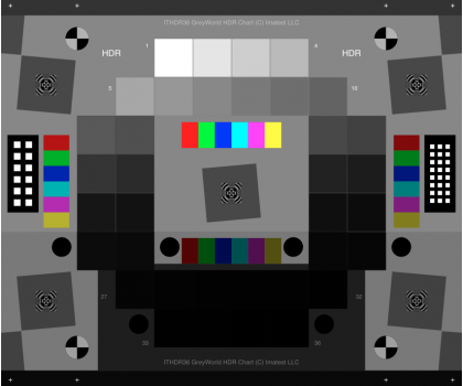
- BETTER — transmissive dynamic range charts, such as an Imatest 36-patch Dynamic Range Test Chart, which has a larger tonal range than reflective charts.
Introduction
Noise is unwanted variations of the measured signal arising from a variety of causes — heat in electronic circuits, photons incident on the image sensor, and many more.
It is usually modeled as a gaussian random process, but noise from photons, called photon shot noise, is a Poisson process (whose statistics strongly resemble a gaussian for mean values over 10 occurrences). Gaussian processes are based on the normal distribution, whose probability distribution function is
\(\displaystyle N(x) = \frac{1}{\sqrt{2 \pi \sigma^2}} \text{exp}\left(- \frac{(x-\mu)^2}{2\sigma^2} \right)\) for mean μ and standard deviation σ.
Noise measurements typically refer to RMS (Root Mean Square) noise, which is equivalent to the standard deviation σ of the signal S.
RMS Noise = NRMS = σ(S), where σ denotes the standard deviation.
S can be the signal in any of several channels: R, G, B, Y (Luminance), or a derived channel such as R-Y or B-Y (both used for chroma noise) or L*, a*, b*, or others.
|
Correcting noise in patches with nonuniform illumination Imatest calculations may deviate slightly from the Noise =σ(S) formulation because the patch used to measure noise may be unevenly illuminated, and this can result in an increase in measured N not actually caused by random noise itself. To account for this we calculate second order fits to the mean signal value in both the x and y-directions, then subtract the second order fits from the signal prior to calculating noise. Hence Imatest noise measurements may be slightly lower than plain standard deviations.
|
Signal-to-Noise Ratio (SNR) is often more useful than the noise itself. It can be expressed as either a simple ratio (SNR = S/N) or in decibels (SNR(dB) = 20 log10(S/N) (familiar to electrical engineers). In digital cameras noise arises from several sources.
- fixed noise (sensor dark current noise and thermal (resistive) noise),
- photon shot noise, which increases with the square root of the mean number of photons striking the pixels,
- Dark Signal Nonuniformity (DSNU), which arises from variations in sensitivity of individual pixels, and
- Photo Response Nonuniformity (PRNU), which arises from variations in the gain of transistors in individual pixels, and increases linearly with illumination
Sensor noise and dynamic range can be measured from raw (completely unprocessed) images, as described in Image sensor noise from raw images.
Settings
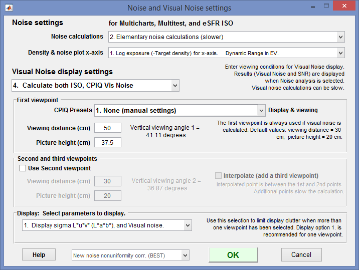
The Noise & Visual noise settings window can be opened from the modules that support detailed noise measurements.
- from Color/Tone Setup, click on Settings, Visual noise settings. (The Visual noise settings window contains several noise settings — not just visual noise.)
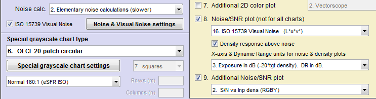
- from Color/Tone Auto, click the Settings button in the Color/Tone Auto Chart area, then press the Noise & Visual Noise settings button. Some settings are also available in the Color/Tone Auto Setup window, a portion of which is shown below.
- from eSFR ISO (run from Rescharts or eSFR ISO Setup), click the More settings button, then the Noise settings button on the left, or click on the Settings dropdown menu, Noise & Visual noise settings…
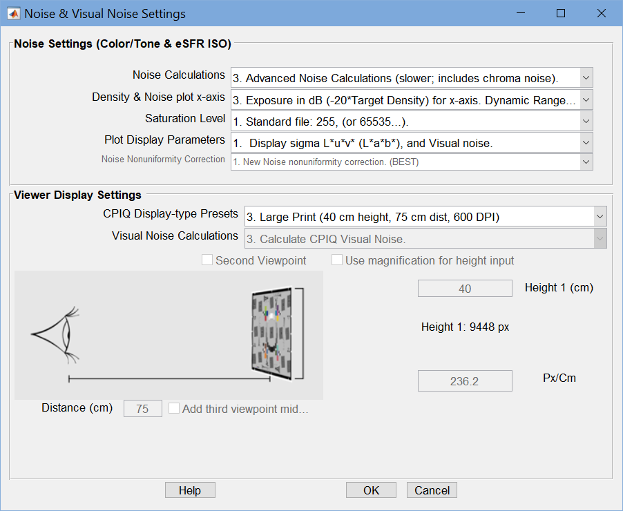 Noise and Visual noise settings, opened by any of the above actions
Noise & Visual Noise settings window
Noise calculations, lets you trade off calculation detail and speed. Choices are
| 1. No (non-visual) noise calculations (fastest) | Use this setting when noise is not needed. |
| 2. Elementary noise calculations (slower) | Includes noise types 1-3 and 10-15 from the table below |
| 3. Advanced noise calculations (slower; includes chroma noise) | Includes noise types 4-9 (Chroma and CIELAB) from the table below. |
Density & noise plot x-axis, lets you select the x-axis for noise plots. Choices are
| X-axis | Dynamic Range Units |
| 1. Log exposure (−target density). | EV. |
| 2. Lux (incident Lux / 10^density). | EV. |
| 3. Exposure in dB (-20×target density). | DdB. |
| 4. Log exposure. | Density units |
| 5. F-stops (EV) | EV (F-stops) |
| 6. 20 Log10(Pixel level (Digital number DN)) | dB |
| 7 Pixel level (Digital number DN) Linear | dB |
Saturation Level — Standard file is recommended for most demosaiced files. Manually-entered is appropriate for most raw files. Details in the dropdown menu.
| Standard file (255 (or 65535 …) | For most demosaiced files |
| ITU-R Rec. 601 (BT. 601) 234 | For the specified video format |
| Maximum detected patch sample | (rarely used) |
| Manually-entered Saturation level | Often used for raw files. Set outside this window. Details in Image Sensor Noise … Saturation level |
Plot Display Parameters — for visual noise-only. Select details of sigma (noise) display.
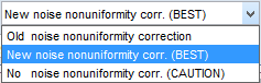
Noise nonuniformity correction — The new calculation is strongly recommended. The alternative is no nonuniformity correction, which may be useful for comparing with external calculations on rare occasions.
Viewer Display Settings
CPIQ Display type Presets — 1. None lets you set Display Height (cm), Display Px/Cm, and Distance (cm). The others are presets for these settings.
-
- None (manual settings, assumed print at 600 DPI)
- Small Print
- Large Print
- Computer Monitor
- 4.5″ Cell Phone
- 30″ 4k UHDTV
Visual noise calculation — selects visual noise calculations, which can be slow.
-
- No Visual noise calculation
- Calculate ISO 15739 Visual noise
- Calculate CPIQ Visual noise
- Calculate both ISO, CPIQ Vis noise
Noise displays
| Color/Tone Setup | Click on 11. Noise analysis (not for all charts) in the noise display options located just to the right of the Settings buttons in and just below the Noise/SNR checkbox. |
| Color/Tone Auto | Open the Settings window (from the Imatest main window or during a Color/Tone run) and select Plots 8 and/or 9 (on the right). (Yes, Color/Tone allows two noise plots because there are so many options.) |
| eSFR ISO (run from Rescharts or eSFR ISO Setup) |
Under Display (on the right) select 16. Noise. Noise Plot (eSFR ISO-only) is available in eSFR ISO Auto. |
Twenty-seven different noise plots are available. All measurements except for 10-12 are for the grayscale patches-only. Settings 10-12 apply to all patches (including color); these are of particular interest for analyzing Image sensor noise from raw images.
| N | Measurement | * | Description |
| 1. | Noise vs. input density (RGB) Noise in pixels or % of maximum pixel level | 2. | Simple noise or SNR derived from standard deviation (σ) of pixel levels. |
| 2. | Signal/Noise (S/N) vs. input density (RGBY) The luminance (Y-channel) is used for S. | ||
| 3. | SNR (dB) vs. input density (RGBY) SNR (dB) = 20 log10(S/N). | ||
| 4. | Chroma noise vs. input density | 3. | Industry-standard chroma noise |
| 5. | Chroma S/N vs. input density | ||
| 6. | Chroma SNR (dB) vs. input density | ||
| 7. | CIELAB (L*a*b*) noise | 3. | Experimental: Seems to make sense since CIELAB is approximately perceptually uniform, but has no industry traction. |
| 8. | CIELAB (L*a*b*) S/N | ||
| 9. | CIELAB (L*a*b*) SNR (dB) | ||
| 10. | Noise vs. pixel (all patches) | 2. | For characterizing image sensor noise. See Image sensor noise from raw images. Less useful with processed RGB images. |
| 11. | S/N vs. pixel (all patches) | ||
| 12. | SNR (dB) vs. pixel (all patches) | ||
| 13. | F-stop (scene-referenced) noise, including Dynamic Range results. | 2. | Used for Dynamic Range calculations |
| 14. | F-stop (scene-referenced) S/N, including Dynamic Range results. |
||
| 15. | F-stop (scene-referenced) SNR (dB), including Dynamic Range results. | ||
| 16. | ISO 15739 Visual noise vs. input density (L*u*v*) | V. | From the ISO 15739:2013 standard. Includes viewing conditions. |
| 17. | ISO 15739 Visual S/N vs. input density (L*u*v*) | ||
| 18. | ISO 15739 Visual SNR (dB) vs. input density (L*u*v*) | ||
| 19. | ISO 15739 Noise and Dynamic Range |
2. | Also from ISO 15739:2013. Completely independent of visual noise. |
| 20. | ISO 15739 Signal/Noise (S/N) and Dynamic Range |
||
| 21. | ISO 15739 Signal-to-Noise Ratio (SNR) in dB |
||
| 22. | CPIQ Visual noise vs. input density (L*a*b*) | V. | From IEEE CPIQ P1858TM (Camera Phone Image Quality) specification. See Imatest CPIQ 2016 Support. |
| 23. | CPIQ Visual S/N vs. input density (L*a*b*) | ||
| 24. | CPIQ Visual SNR (dB) vs. input density (L*a*b*) | ||
| 25 | YUV noise | 3. |
|
| 26 | YUV S/N | ||
| 27 | YUV SNR (dB) |
[ *Notes: 2., 3.: Noise calculation must be set to at least 2 = Elementary or 3 = Advanced;
V. The ISO 15739 Visual Noise checkbox must be checked. ]
Here is a typical noise result for a JPEG image of the X-Rite Colorchecker. The plot shown normalized noise for the grayscale patches (bottom row).

Panasonic GF1, ISO 400
This plot shows noise, in units of percentage of maximum pixel level, for the R, G, B, and Y (luminance) channels for the grayscale patches (in the bottom row for the Colorchecker). 11. Noise plots is selected in the Display area, and the details of the plot (noise measurements and units) are selected below Display. (The noise dropdown menu is where you get to select one of 27 plot choices.)
A checkbox below the button allows you to display tonal response (Log pixel level vs. Input density) above the noise (or S/N or SNR (dB)) plot. Here is a result from a JPEG image of the Imatest 36-patch Dynamic Range chart.)
Dynamic Range and how to measurement is described in great detail on the Dynamic Range page.
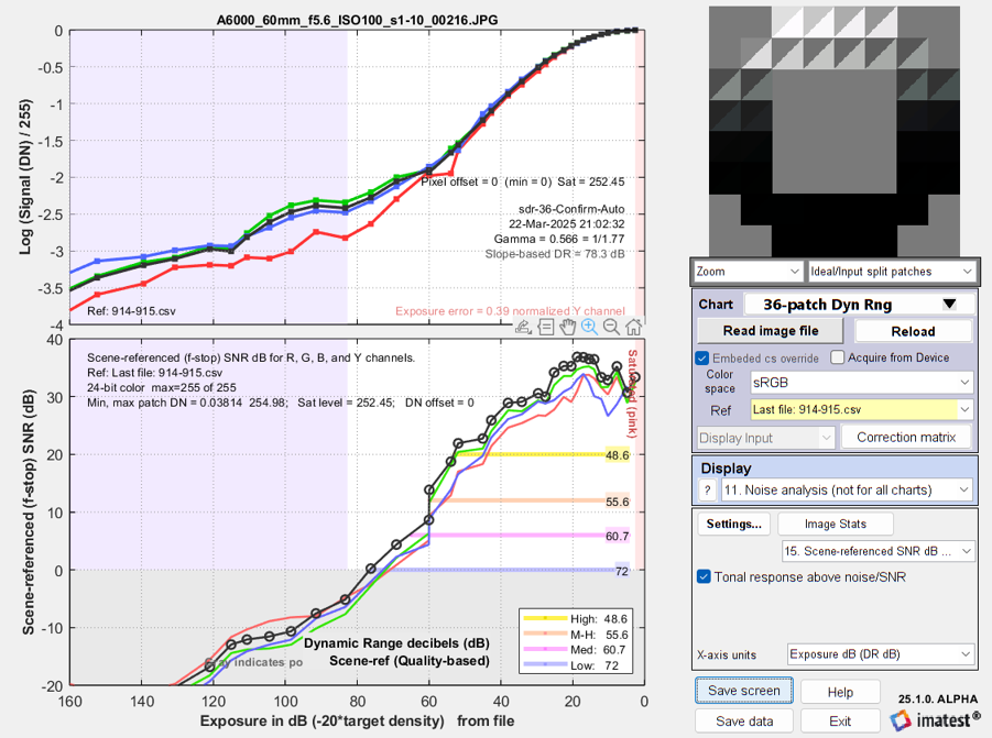
Log pixel level (Tonal Response curve) and Scene-reference (f-stop) noise vs. input density for grayscale patches.
R, G, B, and Y channels. Sony A6000, ISO 100.
The Dynamic Range for this JPEG image seems optimistic because of the strong “shoulder” (low contrast region) on the right. The shoulder is not present in raw image captures, regardless of whether or not they are demosaiced.
Imatest Dynamic range
Dynamic Range (DR) is the range of tones over which a camera responds with good image quality (typically specified by Signal-to-Noise Ratio, SNR) and contrast. It can be measured in f-stops, which are equivalent to zones or EV (factors of two), in decibels (dB), or density units, where one density unit = 3.322 f-stops = 20dB).
It is described in great detail in the Dynamic range page,
Imatest has several types of Dynamic Range calculation, which are cross-referenced here.
| Dynamic range from a single transmissive chart image. | Color/Tone | A transmissive chart is such as the Imatest 36-patch Dynamic Range or HDR chart is required because reflective charts do not have sufficient tonal range. |
| Dynamic range from multiple (differently exposed) images | Dynamic Range module | Uses CSV output of Stepchart of Color/Tone for several differently exposed images. Usually used with reflective charts, but transmissive charts may also be used. |
| ISO 15739 Dynamic Range from patch with density ≈ 2 | Color/Tone, eSFR ISO | Extrapolates Dynamic Range from a single patch with density ≈ 2. |
| Raw image sensor Dynamic Range & characterization | Color/Tone | Described in great detail in Image sensor noise from raw images. Transmissive charts with tonal range ≥ 3 are recommended. |
In Color/Tone (Interactive or Auto), Dynamic Range (based on Scene-Referenced noise or SNR) is defined as density range (in the original scene) over which the scene-referenced RMS noise measured in f-stops (the inverse of the f-stop signal-to-noise ratio, SNR), remains under a specified maximum value and the contrast is adequate. The lower the noise (the higher the SNR, which is the inverse of f-stop noise), the better the image quality. SNR tends to be worst in the darkest regions. Imatest calculates the dynamic range for several minimum SNR levels, from 10 (20 dB; high image quality) to 1 (0 dB; low quality).
-
The dynamic range corresponding to SNR = 1 is closest to the intent of the ISO Dynamic range measurement in section 6.3 of the ISO noise measurement standard: ISO 15739: Photography — Electronic still-picture imaging — Noise measurements. Since the Imatest measurement differs in several details from ISO 15739, the results are close but not identical. They may be compared in the ISO 15739 SNR plots, described below.
Transmission step chart
Several transmission step charts are listed in the Dynamic Range page. In this page, we focus on the recommended Imatest 36-patch Dynamic Range charts. which come in several variants with density step of approximately 0.1 in light regions and maximum densities of approximately 3.6, 6, and 8.2.
A nearly circular patch arrangement ensures that light falloff (vignetting) has minimal effect on results. A CSV or CGATS reference file with actual densities is required (An individually-measured density file is supplied with each chart.) the chart has an active area of 7.75×9.25 inches on 8×10 inch color film.
It also contains slanted edges in the center and corners with 4:1 contrast for measuring MTF. The edges have an MTF50 >= 16 cycles/mm, which is about 3 times better than the best inkjet charts. Registration marks make the regions easy to select, and fully automated region detection is available in Color/Tone. A neutral gray background helps ensure that the chart will be well-exposed in auto exposure cameras (compared to charts with black backgrounds, which are sometimes strongly overexposed). Darker backgrounds and masks are available.
Single-layer 36-patch Dynamic Range charts can be used with the Dynamic Range postprocessor to measure dynamic ranges larger than 11 f-stops if several manual exposures are available. But we don’t generally recommend this because the important effects of veiling glare (flare or stray light) are not measured.
 Imatest 36-patch Dynamic Range chart Imatest 36-patch Dynamic Range charton 8×10 film. Dmax ≈ 3.4. |
 Imatest 36-patch High Dynamic Range (HDR) chart Imatest 36-patch High Dynamic Range (HDR) charton 8×10 film. Dmax ≥ 6.0. |
This chart is produced with a high-precision LVT film recording process for the highest density range, lowest noise, and finest detail. The HDR chart on the right has one or two extra layers covering the bottom 14 patches.
Lightbox
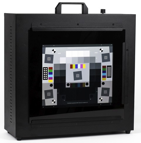 You’ll need a lightbox that can evenly illuminate the transmission step chart. 9×12 inches is large enough in most cases. Avoid thin or “mini” models, which may not have even enough illumination. Our lightbox product lineup is frequently updated.
Imatest lightboxes and other uniform light sources are listed here.
A typical Imatest LED Lightbox (shown on the right), Imatest lightboxes have several attributes.
- Highly uniform illumination.
- High-quality spectral response. You to choose color temperatures, typically 3100K, 4100K, 5100K, 5500K, and 6500K color temperature with a Color Rendering Index (CRI) of 97. NIR channels of 850nm and 940nm are available. The box comes with a multi-channel mix mode so you can mix a combination of channels for a continuous range of color temperatures.
- Intensity is adjustable via a hardware knob, WIFI, or USB from 30-10,000 lux: a range of over 300:1, making it suitable for measurements from near-daylight to extremely dim light.
To measure dynamic range, read the detailed instructions on Dynamic Range, which are summarized below.
- Place the chart on the lightbox— or any source of uniform diffuse light. Be sure to block direct light from the lightbox outside of the chart: Stray light can reduce the measured dynamic range; it should be avoided.
- Photograph the chart in a darkened room. No stray light should reach the front of the target; it will distort the results. The surroundings of the chart should be kept as dark as possible to minimize flare light.
- The chart does not need to fit the frame.
- Use your camera’s histogram to determine the minimum exposure that saturates the lightest region of the chart. Overexposure (or underexposure) reduces the number of useful zones. The lightest region should have a relative pixel level of at least 0.98 (pixel level 250 or 255); otherwise, the full dynamic range of the camera will not be detected. If the lightest zone is below this level, and a transmission chart is selected, a Dynamic range warning is issued.
- Photograph the chart following instructions in Using Color/Tone Interactive or Using Color/Tone Auto.
The dynamic range is the difference in density between the zone where the pixel level is 98% of its maximum value (250 for 24-bit color, where the maximum is 255), estimated by interpolation, and the darkest zone that meets the measurement criterion. The repeatability of this measurement is better than 1/4 f-stop.
Imatest Dynamic range results
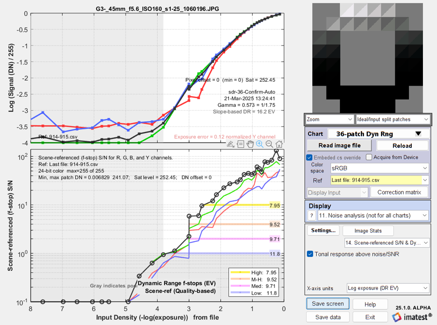
Here are results for the Panasonic G3 (a Micro Four-Thirds camera with 3.75 micron pixel pitch) at ISO 160, converted from raw using LibRraw with the following settings: Demosaicing: Normal RAW conversion (demosaiced), Output gamma: 2.2, White Balance: Camera, Output color space: 48-bit, Quality: Default.
|
|
Same image capture, |
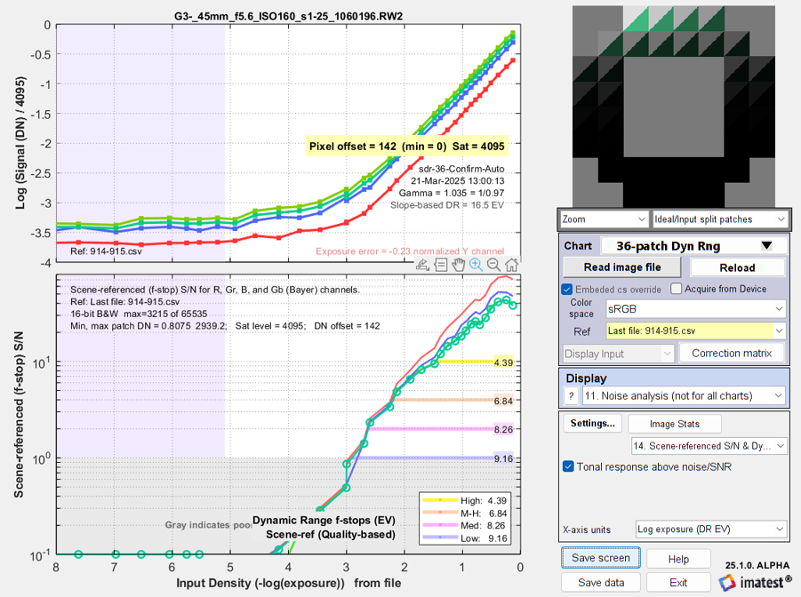
The Dynamic Range at low-quality level (scene-referenced SNR = 1) is 9.16 f-stops, decreasing to 4.39 f-stops at high-quality level (SNR = 10). These results are unchanged for 24-bit raw conversion.
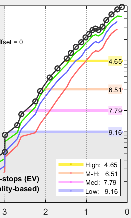
The shape of the response curve is a strong function of the conversion software settings. The plot below is for the same exposure, saved as a JPEG file inside the camera. Note that the transfer curve is quite different: it has a “shoulder” in the highlights, which improves pictorial quality by reducing the tendency of highlights to saturate (“burn out”). Dynamic Range is improved due to software noise reduction (absent in the LibRaw conversion).
Panasonic G3, ISO 160, in-camera JPEG. Note the “shoulder.”
Dynamic range is improved due to software noise reduction.
Several options are available in the Display area and in the Settings window for selecting x and y-axis units. To convert dynamic range from f-stops into decibels (dB), the measurement normally given on sensor data sheets, multiply the dynamic range in f-stops by 6.02 (20 log10(2)). The dynamic range for low quality (f-stop noise = 1; SNR = 1) corresponds most closely to the number on the data sheets. Measured dynamic range is often lower than specified sensor dynamic range because of lens flare and other factors.
The presence of a strong shoulder in the highlights—where the slope of the transfer curve decreases to near-zero, or flat—indicates a loss of contrast in the highlight regions. The shoulder may have some pictorial advantages: it reduces highlight “burnout”.
Quality-based dynamic range calculations are limited by the slope of the transfer curve in the highlight regions. Shoulder regions of the transfer curve where the slope is less than 0.05 (near-zero) do not contribute to the quality-based dynamic range. On noise analysis displays with quality-based dynamic range values, this manifests as a gap between the saturation region and the High/M-H/Med/Low quality level bars, as shown below.
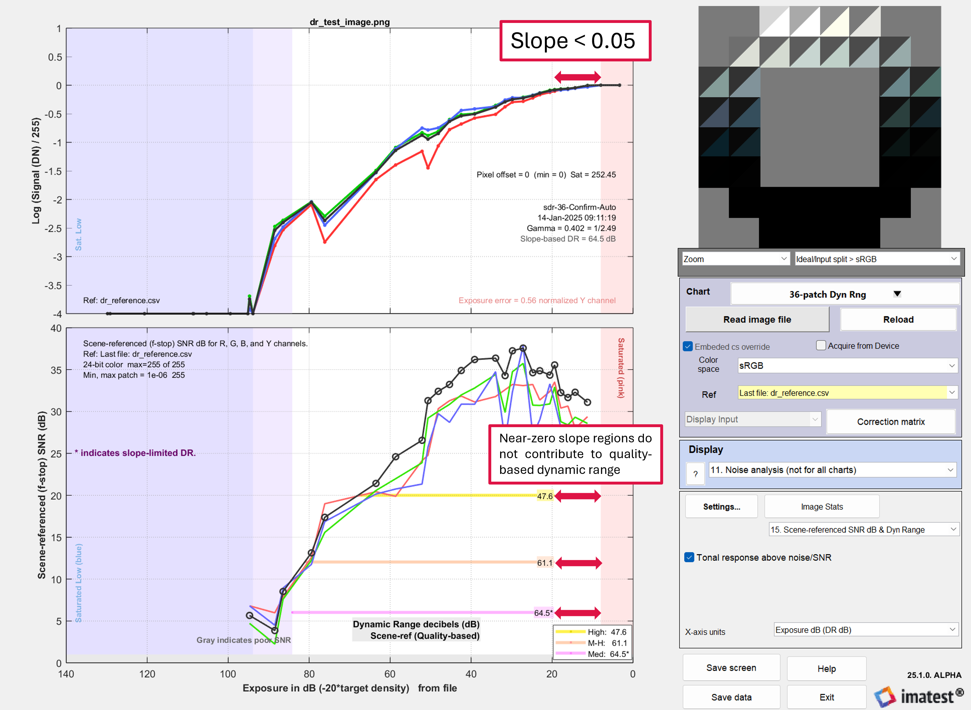
Shoulder regions of the transfer curve with near-zero slope indicate a severe loss of contrast in the highlights,
and therefore do not contribute to dynamic range.
Image sensor (RAW) noise and dynamic range
|
Documentation on RAW image sensor noise has been moved to Image Sensor Noise – measurement and modeling because it’s a large subject and critical for Simatest simulations. |
A remarkable property of raw (unprocessed) images is that the noise in a patch of identically-illuminated pixels is a function of the pixel level (or Digital Number, DN), regardless of color.
As a result of this property, raw images have two important uses.
- Measure sensor dynamic range, which is distinct from camera dynamic range, which is limited by stray light (flare, veiling glare) from the lens.
- Characterize sensor properties, which can be used in the ISP (Image Signal Processing)/Camera simulator, Simatest, which can be used to explore system performance as a function of exposure, Exposure Index (system gain), (relative) light level, sharpening, noise reduction, and more.
Table of contents of Image Sensor Noise – measurement and modeling
- Introduction
- Experimental technique — Good technique for working with transmissive grayscale (dynamic range) charts
- Raw file types — Commercial vs. binary files (usually from development systems)
- Reading commercial raw files — Using LibRaw
- Reading custom (binary) raw files — Using Generalized ReadRaw
- Processing the Bayer raw image — Bayer raw image formats (RGGB, etc.) and how to use the Standard monochrome or Bayer raw? window
- Black level offset and saturation level — describes how the black level offset, DNmeas , which remains in undemosaiced images, is estimated and removed. Also describes the maximum Digital Number, DNmeas, which is also handled differently for undemosaiced files.
- Image sensor noise model — equations
- Run Color/Tone and calculate additional results
- Dynamic Range — Measuring sensor Dynamic range from raw images
- EMVA 1288 measurements
- Closing the loop: comparing measured and simulated performance
- Summary
- Appendix 1. Direct DNG read of commercial raw files
- Appendix 2. Algorithms
Image sensor equations
Many “raw” (undemosaiced) images are not perfectly raw. The measured digital number, DNmeas , frequently includes a black level offset, DNoff , added to prevent noise at low signal levels from clipping and distorting the mean signal level, which makes it difficult to detect dead pixels. The offset may include veiling glare (flare light), which should be kept to a minimum with good experimental design, as described in How to measure dynamic range.
Most raw (undemosaiced) files from commercial cameras contain the black level offset (or “pedestal”) as well as a maximum (saturation) pixel level, often 2N-1 for N-bit Analog-to-Digital converters (ADCs), which is lower than the maximum level for the file format, for example, 4095 of 65535 for a 12-bit ADC in a 16-bit file format.
The LibRaw program we use for processing raw files removes the offset and normalizes the maximum level when files are demosaiced (converted to RGB), but does not remove the offset or saturation level when the output is not demosaiced (kept as Bayer raw).
The Digital Number at the image sensor is
DN = DNmeas – DNoff
The black level offset, DNoff —what it is and how to estimate and remove it, is discussed in great detail in Image sensor noise — lack level offset and saturation level.
The noise equations, which are presented in great detail in Image sensor noise model — equations, will be briefly summarized here.
The normalized signal at the image sensor, used in the equations, is
V = DN / DNmax
where DNmax is the maximum allowable Digital number for the sensor, which is normally 2B-1 for demosaiced RGB signals with bit depth = B (256 for B = 8 or 65535 for B = 16). Programs that demosaic images typically normalize DN to this level, but images processed without demosaicing, so the data is unchanged from raw data, are usually not normalized. For files with bit depth = B = 16 and ADC (Analog-to-Digital Converter) precision a < 16, DNsat is often lower (2a-1 ): 4095 for a = 12 or 16383 for a = 14, although the values may be different. Saturation level is described is Black level offset and saturation level.
The noise model used as input to Simatest is derived from two sources: the book, “Photon Transfer DN → λ” by James R. Janesick and the EMVA 1288 standard. The expected (modeled) noise (standard deviation) is
\(\sigma_N = \sqrt{k_{Ndark}^2 + k_{Nshot}^2 V + k_{FPN}^2 V^2}\)
where
σN(V) is the total image sensor noise amplitude (the standard deviation of the noise voltage),
expressed as a function of the normalized signal V. σN2(V) is the variance (or power).
kNdark is the coefficient of the dark noise, or equivalently, the dark noise amplitude. k2Ndark is the dark noise power.
kNshot is the coefficient of the photon shot noise.
kFPN is the coefficient of the Fixed-Pattern Noise (derived from PRNU).
Image Sensor Noise – measurement and modeling contains instructions on how to
- read the two types of raw file — commercial and binary (from development systems).
- handle measurement issues, such as determining and adjusting the maximum (saturation) level and removing the black level offset,
- measure dynamic range, and
- build an image sensor model using Simatest that can be used to predict the performance of a wide variety of imaging systems.
Temporal noise
Temporal noise— noise that varies independently from image to image, with fixed-pattern noise removed— can be calculated by two methods
- the difference between two identical test chart images (the Imatest recommended method), and
- the ISO 15739-based method, which where it is calculated from the pixel difference between the average of N identical images (N ≥ 8) and each individual image.
Note that fixed pattern noise can be calculated by selecting Combine files for signal averaging.
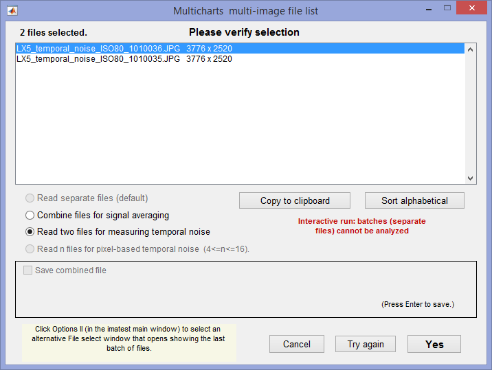
(1) Difference method. In any of the modules, read two images. The window shown on the right appears. Select the Read two files for measuring temporal noise radio button.
The two files will be read and their difference (which cancels fixed pattern noise) is taken. Since these images are independent, noise powers add. For independent images I1 and I2, temporal noise is
\(\displaystyle \sigma_{temporal} = \frac{\sigma(I_1 – I_2)}{\sqrt{2}}\)
In Color/Tone, temporal noise is displayed as dotted lines in Noise analysis plots 1-3 (simple noise, S/N, and SNR (dB)).
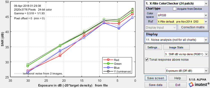 SNR (dB) for Colorchecker chart: temporal noise shown as thin dotted lines.
(2) Multiple file method. From ISO 15739, sections 6.2.4, and 6.2.5. Currently we are using simple noise (not yet scene-referred noise). Select between 4 and 16 files. In the multi-image file list window (shown above) select Read n files for temporal noise. Temporal noise is calculated for each pixel j using
\(\displaystyle \sigma_{diff}(j) = \sqrt{\frac{1}{N} \sum_{i=1}^N (X_{j,i} – X_{AVG,j})^2} = \sqrt{\frac{1}{N} \sum_{i=1}^N X_{j,i}^2 – \left(\frac{1}{N} \sum_{i=1}^N X_{j,i}\right)^2 } \)
The latter expression is used in the actual calculation since only two arrays, \(\sum X_{j,i} \text{ and } \sum X_{j,i}^2 \), need to be saved. Since N is a relatively small number (between 4 and 16, with 8 recommended), it must be corrected using formulas from Identities and mathematical properties in the Wikipedia standard deviation page. \(s(X) = \sqrt{\frac{N}{N-1}} \sqrt{E[(X – E(X))^2]}\).
\(\sigma_{temporal} = \sigma_{diff} \sqrt{\frac{N}{N-1}}\)
We currently recommend the difference method (1) because our experience so far has shown no advantage to method (2), which requires many more images (N ≥ 8 recommended), but allows fixed pattern noise to be calculated at the same time. There is a detailed comparison of the methods in Measuring Temporal Noise.
Chroma noise
Two types of chroma noise display are available.
Standard ISO-based chroma noise. Displays 4-6 show the noise and SNR for the Y (Luminance), R-Y, and B-Y channels as well as total noise using two different weightings. The total weighted noise used in the ISO 12232-2006 and ISO 15739-2013 standards (based on the paper, ISO 12232 revision: determination of chrominance noise weights for noise-based ISO calculation (http://dx.doi.org/10.1117/12.582447) by Sean Kelly and Brian Keelan) is plotted as a solid black line (with ◊ markers). Total weighted noise is σ(D) = [ σ(Y)2 + 0.279 σ(R-Y)2 + 0.088 σ(B-Y)2 ]1/2. The older total weighted noise ([ σ(Y)2 + 0.64 σ(R-Y)2 + 0.16 σ(B-Y)2 ]1/2) used in ISO 12232:1998 and 15739-2003 is obsolete and may be deprecated in a future Imatest release.
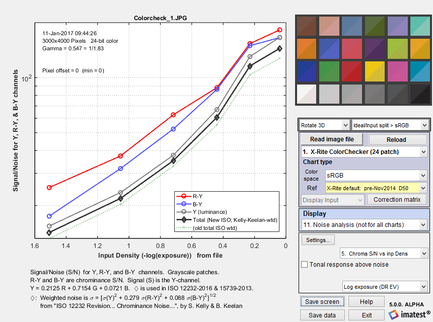 Signal/Noise for R-Y and B-Y (chroma) and Y (Luminance) channels,
 as well as Total weighted noise from SO 12232-2006 and ISO 15739-2013 (—◊—).
L* a* b* (CIELAB) noise is potentially interesting because CIELAB was designed to be a perceptually-uniform space. Although it is less uniform than intended— which is why color difference metrics like ΔE-2000 were developed— it is still much more uniform than many other representations, such as RGB. CIELAB noise is not a standard measurement. There is very little literature on using CIELAB for noise measurements. even though a* and b* might be a better measure of chroma noise than R-Y and B-Y (above). We are not aware of any weighting factors (for combining L*, a*, and b* into a single number).

ISO 15739 and CPIQ Visual noise
Imatest 4.0+ includes a calculation of ISO 15739 visual noise as specified in Appendix B of the ISO 15739:2013 standard. And Imatest 4.4+ includes a calculation of visual noise from the IEEE CPIQ P1858 (Camera Phone Image Quality) 2016 specification, which is based on ISO 15739 with some added details. These are relatively complex calculations that include the effects of the human visual system. It is performed for all grayscale patches for up to three viewing conditions (viewpoints), each of which is specified by viewing distance and display (picture) height. The vertical display angle (in degrees) is
Viewing angle = 360/pi*atan(.5*picture height/viewing distance)
We summarize the calculation in the table below. Details can be found in the ISO 15739:2013 standard, Appendix B and in the IEEE CPIQ P1858 (Camera Phone Image Quality) 2016 specification.
| ISO | CPIQ | Step | Description |
| B.2.1 | D.1 D.2 |
RGB to XYZ(E) | Convert RGB to XYZ values for illuminant E, typically by converting RGB to XYZ(D65), then converting from XYZ(D65) to XYZ(E). Though the standard specified sRGB color space (the Windows/internet standard), Imatest can work with any color space. See en.wikipedia.org/wiki/CIE_1931_color_space. |
| B.2.2 | D.4 | XYZ(E) into opponent space AC1C2 | A relatively straightforward matrix operation. |
| B.2.3 | Discrete Fourier Transform | Transform A, C1, C2 into Fourier space (cycles/pixel). | |
| B.2.4 | D.6 | Apply the contrast sensitivity function (CSF) | There are three functions: for A (identical to luminance Y), C1, and C2. Viewing conditions are used here (f in cycles/degree is calculated from the vertical pixel count and angle). |
| D.7 | Apply Display/Printer MTF. | ||
| D.8 | High Pass FIlter (HPF) | Cutoff < 1 cycle/degree. DC (calculated prior to the filter) is restored after the filter. | |
| B.2.5 | Inverse Fourier Transform | Back to A, C1, C2. | |
| B.2.6 | D.10 | Opponent space AC1C2 into XYZ(E) |
A relatively straightforward matrix operation. |
| B.2.7 | XYZ(E) to XYZ(D65) | Another relatively straightforward matrix operation. | |
| B.2.8 | XYZ(D65) to L*u*v* | CIELUV (L*u*v*) is a relatively perceptually uniform color representation that remains relatively unfamiliar. L* is nonlinear: proportional to brightness to the 1/3 power. Note that this is a filtered space (not plain L*u*v*). | |
| D.12 | XYZ(D65) to L*a*b* (CIE Lab) |
Numbers seem to be similar to the L*u*v* numbers from ISO 15739. | |
| B.2.9 | Standard deviation for each grey patch | The noise for each (L*, u*, v*) channel is the standard deviation of the levels for the patch. | |
| B.2.10 | Weighted sum representing the visual noise | V = σL* + 0.852 σu* + 0.323 σv* | |
| D.13 | Objective noise (CPIQ) | Ω = log10[1 + 23.0 σ2(L*) + 4.24 σ2(a*) – 5.47 σ2(b*) + 4.77 σ2(L* a*) |
Rube Goldberg would have been impressed. His spirit is with us.
Noise settings window
To adjust visual noise settings
- In Color/Tone Interactive, click Settings… (on the right). This opens the Color/Tone Settings window, which has a Noise & Dyn Rng section in the middle that contains several settings. Click on Visual noise settings.
- In Color/Tone Auto, open the image, then press Continue (not express), or from the Imatest main window, click Settings (just below the Color/Tone Auto chart selection), then click Noise & Visual noise settings.
- In eSFR ISO (run from Rescharts or eSFR ISO Setup), click the More settings button, then the eSFR ISO Noise settings button, or click on the Settings dropdown menu, Noise & Visual noise settings…
These selections open the Noise and Visual Noise Settings window, shown on the right.
Noise Settings (Color/Tone…) near the top are for noise in general.
Except for Plot Display Parameters, settings are repeated from the Settings window.
- Noise Calculations – refers to non-visual noise: 1. None (fastest), 2. Elementary, and 3. Advanced (slowest). 2. Elementary is a good choice for most applications.
- Density & Noise plot x-axis – is relatively self-explanatory
- Saturation level – is significant when the saturation differs from the maximum for the bit depth (65535 for bit depth = 16, etc.), for example, when 12-bit data is stored in a 16-bit file.
- Plot Display Parameters – lets you choose which of the results (combinations of L*, u*, v*, and Visual noise) to display. When all are chosen, the plot is cluttered.
- Noise nonuniformity correction – Setting 1 is recommended because it compensates for nonuniform illumination, so it isn’t mistaken for noise.
Viewer Display Settings are for Visual noise.
Visual noise requires a viewpoint, which consists of display height, viewing distance, and device resolution in pixels/cm. The viewing angle is calculated from the distance and height.
Older noise settings (no longer active)
CPIQ Display-type Presents contains 6 settings:
1 is for None (manual settings; no preset). You need to enter the viewpoint (Height, Px/CM, Distance Cm), and you can add one or two additional viewpoints. If a second viewpoint has been entered, you can select a third, which will be halfway between the first two viewpoints. You can also select Visual Noise Calculations, which is disabled (always set to 3. CPIQ) for presets 2-6.
2-6 are presets for a for several displays: 2. Small print, 3. Large print, 4. Computer monitor, 5. Small cell phone, and 6. UHD TV. Details are in the dropdowns. Height, Px/Cm, and Distance are disabled and contain the preset settings. Visual Noise Calculations is set to 3. Calculate CPIQ Visual Noise, even if the input setting is different. Use 1. None (…) to select a different setting or keep the input setting.
Because visual noise is expressed as the standard deviations of the L*, u*, and v* channels, whose scaling is unfamiliar to most engineers and scientists, Imatest offers three displays of visual noise: one of the noise itself and two of signal-to-noise ratios (expressed as a fraction and as decibels (dB)).
16. ISO 15739 Visual Noise (L*u*v*)
17. ISO 15739 Visual S/N (L*u*v*) S/N (Signal-to-Noise Ratio, as a fraction)
18. ISO 15739 Visual SNR dB (L*u*v*) SNR dB (Signal-to-Noise Ratio in decibels (dB) = 20*log10(fraction))
We present two examples. The first is for an X-Rite Colorchecker for three viewpoints. All results are presented. (The plot is somewhat cluttered, but still readable).
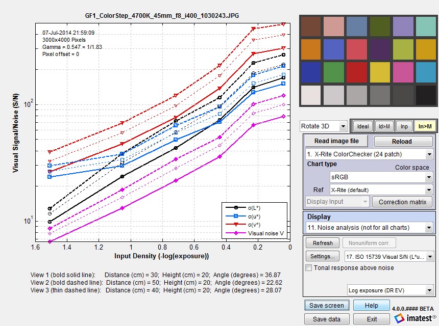 Visual SNR (Signal / Noise) for three viewpoints for an X-Rite Colorchecker.
On the y-axis, 101 corresponds to 20 dB; 102 corresponds to 40 dB.
The second example shows L* noise (σL*) and total visual noise (V) for the same three viewpoints for the Imatest 36-patch Dynamic Range chart. The absolute numbers are somewhat difficult to interpret due to their unfamiliarity: that’s why Imatest also displays Signal-to-Noise Ratios (as fractions and in dB). Noise levels for input densities above (to the left of) 2.0 or 2.5 have little meaning because the image is nearly black (though these levels may be increased by tone-mapping or digital “dodging”).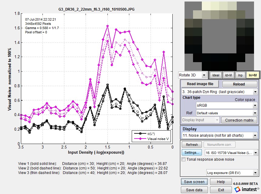 Visual noise for three viewpoints for the Imatest 36-patch Dynamic Range chart.
ISO 15739 SNR and Dynamic Range
The ISO 15739 Dynamic Range (DR) calculation allows DR to be estimated from a patch with density = 2.0, which is available on many semigloss reflective test charts (though density = 2— where 1/100 of the incident light is reflected— cannot be achieved with matte media. The response is fairly accurate for standard (linear) sensors, but is not suitable HDR (High Dynamic Range) sensors. It does not take the effects of flare light into account.
Notes on ISO 15739 SNR and Dynamic Range calculations
- These calculations, which are described in sections 6.2 and 6.3 and Annex D of the ISO 15739:2013 Standard, are completely independent of the ISO 15739 Visual Noise measurements, described in Annex B.
- Imatest’s ISO 15739 SNR calculation is primarily for total SNR (§6.2.3). Temporal noise and SNR have been added in Imatest 5.1. There are two calculation methods: (1) from the difference of two images (divided by √2) and (2) from multiple images (typically 8), following ISO 15739. We recommend method (1) (difference of two images), which is faster and equally accurate. Fixed pattern noise can be measured by averaging at least 8 identical images (by reading multiple images and specifying signal averaging).
|
The definition of Signal-to-Noise Ratio (from §6.2.3-6.2.5 and Annex D of the ISO 15739 Standard) is SNR = Q = g L / σ where σ = noise in pixels, L = luminance (linear), and g is the first derivative of the OECF (the pixel level I vs. luminance curve). g = dI/dL Luminance L is derived from test chart patch density d (which is equal to (-)log exposure): L = 10–d. The numeric formula for calculating g is given in Annex D. (Pixel level I and Luminance L are smoothed prior to calculating g, with a kernel of 3 or 5 points for <7 or ≥7 patches, respectively.) Though it isn’t obvious from the standard, L must be scaled (multiplied) by reference luminance Lref, as defined in §6.2.2. The definition of Lref is not entirely self-consistent, but it appears that Lref is the luminance that corresponds to a linear pixel level of 91% of the clipping level. For gamma-encoded images with bit depth N, where gamma (γ) is measured from the grayscale patches in the image, this corresponds to a pixel level of Iref = (2N-1)*0.91γ . For standard color space (sRGB) images where γ ≅ 1/2.2 = 0.4545 and N = 8, Iref = 255*0.91(1/2.2) = 244.3 This is close enough to the pixel value of 245 cited in the standard. If the maximum grayscale pixel level is greater than Iref, Lref can be found by interpolation. If the maximum grayscale pixel level is lower than Iref, the pixel curve is extended using the measured value of gamma, to find Lref. SNR (Q) is reported at a luminance of 0.13*Lref. This SNR value and the corresponding input density are reported as Dynamic range is defined as DR = Lsat/Lmin where Lsat is the saturation luminance (we take the luminance where pixel level = 0.995 of saturation), and Lmin is the luminance where SNR = 1. Since this low SNR level may not be reached (especially with reflective charts) the standard allows Lmin to be estimated (by extrapolation) as Lmin = σ(d=2)/g(d=2). Though we trust this calculation less than a direct measurement, we have found that is it very close in practice. In the plot below (for a JPEG image from the Panasonic G3 at ISO 160), DR(d=2.04) = 3.31 density units; DR(SNR=1) is not measured because the minimum SNR > 1. The Imatest (1/f-stop) scene-referenced DR, shown above (plot 14), is approximately 3.5 (SNR comes very close to 1). |
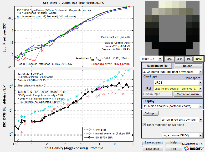
ISO 15739 SNR (S/N) for the Imatest 36-patch Dynamic Range chart.
Plain pixel S/N (plot 2) in Cyan; Imatest (f-stop) scene-referenced S/N (plot 14) in Red.
The large magenta diamond ♦ (above) is located at luminance level \(L_{SNR} = 0.13 \times L_{ref}\), specified for measuring Signal-to-Noise Ratio (SNR) in the ISO standard §6.2.2, equation (4). Lref is the luminance corresponding to pixel level 245 (of 255 for bit depth = 8), i.e., a little below saturation. 0.13 corresponds to 17.7 dB (0.886 Optical Density).
When ISO 15739 SNR is displayed in Color/Tone, or eSFR ISO, it is compared with the older Imatest f-stop-based calculation. Dynamic Range results tend to be fairly similar. The ISO calculation has two advantages. 1. It conforms to a standard and 2. it allows Dynamic Range to be calculated from SNR for a patch with density near 2— which is achievable with (semigloss) reflective media. This calculation uses extrapolation, which is less direct than finding the density where SNR = 1 (which generally requires transmissive media or several exposures). But in our experience, it produces useful results that are close enough to the direct measurement for practical work, i.e., for comparing different cameras in a standardized way.