Gamutvision main page – Gamutvision Table of Contents/Site map – Using Gamutvision – Using Gamutvision 2: Displays
Structure – Getting started – Test pattern – Table of displays – Menu settings – Tips
Gamutvision™ is a powerful utility for exploring color management. With it you can
- Examine color space and device gamuts (ranges of reproducible colors).
- Study gamut mappings and rendering intents (image transformations between color spaces or devices with different color gamuts and algorithms for handling colors where input colors are near or outside the output gamut). The definitions of the four rendering intents can be quite vague— especially perceptual rendering intent, which is often recommended for photographers— and may not correspond to actual performance.
- Evaluate ICC profile quality.
- Estimate printer and paper quality by examining ICC profiles— which you can download from the Internet.
- Preview how much an image or simulated X-Rite™ ColorChecker® will change when sent to a printer.
| Gamutvision 2.0 will be available as a module in Imatest (Studio and Master) in the Imatest 23.1 Pilot program in late October 2022. It may be released as a standalone program if there is sufficient customer interest. |
Gamutvision uses ICCTrans, the Matlab interface to the LittleCMS color management system. The ICCTrans source code is on Github. The ICCTrans manual may have disappeared from the Internet, so we’ve put it on the Imatest website. Many thanks to Ignacio Ruiz de Conejo and Marti Maria (of Hewlett-Packard Spain) for their outstanding work.
Gamutvision structure
Gamutvision analyzes
- one of several built-in test patterns that represent the extremes of available color gamut (and can be adjusted to display reduced gamuts),
- external image files,
- a simulated X-Rite (Calibrite) ColorChecker®.
- a L*a*b* test chart reference file created by Imatest Test Charts — transforming it into a reference file that correctly represents the printed chart.
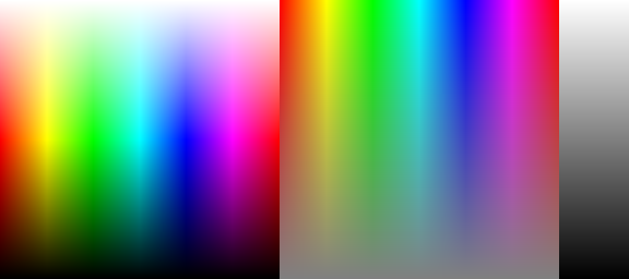
The test pattern is displayed on the upper-right of the Gamutvision window. The two built-in color test patterns vary HSL Hue H and either Lightness L or Saturation S, keeping the third parameter (S or L) fixed. HSL values include (HSL) in their designation to distinguish them from CIELAB, e.g., L(HSL) vs. L*.
|
Basic built-in patterns
 |
||
| Left: Fixed saturation S(HSL) pattern (normally S(HSL) = 1) with all HSL Hues and Lightnesses. Represents the gamut boundary when Saturation S(HSL) = 1 (its maximum value). S(HSL) can be reduced (< 1) to visualize profile behavior for unsaturated colors. | Middle: Fixed lightness L(HSL) pattern (normally L(HSL) = 0.5) with all HSL Hues and Saturations. Colors reach maximum saturation at Lightness L(HSL) = 0.5. L(HSL) can be selected, 0.05 ≤ L(HSL) ≤ 0.95. | Right: Grayscale pattern. 0 ≤ L(HSL) ≤ 1. |
|
The diagram on the right illustrates Gamutvision’s data flow in detail. RGB input consists of one of the patterns shown above or an external image file. To obtain the input display it is mapped to L*a*b*, xy, or uv using the input profile. RGB input is also mapped from the input to the output profile to obtain the output RGB (or CMYK) values, which are then mapped to L*a*b*, xy, or uv using the output profile to obtain the output display. Numerous display options are available. |
 |
|
Here is a broader picture Gamutvision’s structure. You can select up to four ICC profiles: two input profiles and two output profiles.
|
 |
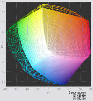
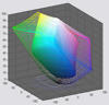
For example, to compare the effects of two working color spaces with a single printer/profile combination, you would enter the two working color space profiles into input Profiles 1 and 3 and the same printer profile into output Profiles 2 and 4. You could then view profiles 1 and 2 or 3 and 4 (showing the effects of the gamut mapping), or you could use a Display box (A or B, shown below) to compare the output gamuts in profiles 2 and 4. The gamuts for Epson R2400 Premium Luster prints made from Adobe RGB (1998) (wireframe) and sRGB (solid) working color spaces are shown on the right, using the 3D L*a*b* display set to . (Displays on this page use Epson-supplied X-rite “premium” profiles, released around October 2005; different from earlier profiles supplied with the R2400). |
 |
Getting started
Gamutvision is opened from Imatest in the Utility dropdown or Misc. tab (on the right) of the classic user interface. If it is released as a separate program, it will be opened in a similar manner to Imatest.
When you open Gamutvision the following window appears. The first time you run Gamutvision, Browse… appears in all four profile windows (bottom left). Settings are saved in succeeding runs.
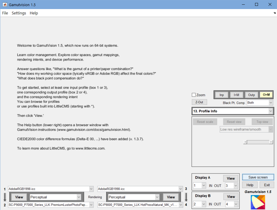 Gamutvision opening (welcome) window
|
Browse… *sRGB (IEC6 1996-2.1 sRGB) *Lab (D50-based Lab) *LabD65 (D65-based Lab) *XYZ (XYZ (D50)) *Gray22 (D50 gamma=2.2 grayscale) (previous profile) Profile and output from box 2 (for Profile 3 only) Recent ICC profile |
|
The Browse… dialog box shown on the right opens by default in the Windows XP profiles folder. If you are using a different system, you should first click on Settings, ICC profile folder and navigate to the appropriate folder. The folder may contain a large variety of profiles– for scanners, cameras, printers, monitors, etc. You will normally select source or display (color space) profiles (not output) for input profiles (1 and 3) and display or output (often printer) profiles for output profiles (2 and 4). |
 |
- Click on
 on the right the Profile 2 popup menu, located at the lower left of the Gamutvision window, just below . The same options appear as for the Profile 1 popup menu. Select a profile.
 - To change the rendering intent, click on the rendering intent menu, between the Profile 1 and Profile 2 popup menus, to the right of . You can choose among
- the four classic rendering intents: Perceptual, Colorimetric (relative), Saturation, or Absolute (colorimetric),
- None, in which case no gamut mapping takes place, and the full gamut of the output profile is displayed,
- Round trip (Perceptual or Colorimetric), useful for evaluating printer profile quality. Described here, and
- the four classic rendering intents, soft-proofed (previewed on the monitor). Soft-proofed gamuts are restricted by the monitor profile’s gamut. The monitor profile, which defaults to sRGB, can be selected by clicking Settings…, Monitor profile. These intents enable soft-proofed monitor gamuts to be compared with final output.
- Select the desired view in the main display selector. 3D L*a*b* (wire input, solid output), shown below, is a good view to start with. You can freely switch between views at any time.
- Now, click on to see the results of the gamut mapping from input profile 1 to output profile 2.
- You may repeat steps 1 through 5 for Profiles 3 and 4. You can chain profiles by selecting Profile 2 (output) as the input for Profile 3. Displays A and B allow input and output profiles to be compared side-by-side.
|
The full Gamutvision window is shown reduced below. Explanatory tooltips appear when the cursor is moved over buttons or controls.
| The large image on the upper left contains the primary gamut display. The 3D L*a*b* plot of the input gamut (wire frame) and mapped output gamut (solid) is shown. You can change the angle of view by clicking your left mouse button anywhere on the image, then moving it. You can also zoom in and out and select among several other options. The gamut volume, which is the single number that best characterizes color response, is shown on the lower right of the gamut display. Several additional views, listed in the table below, can be selected from the display selector box on the right that contains 3D La*b* (wire input, solid output). | The image on the right contains the test pattern or image. Depending on the settings (, …, ), the input or output image may be displayed in its original form or mapped to the monitor color space (typically similar to sRGB). Settings are described in the table below. Output mapped to display profile is the default. |
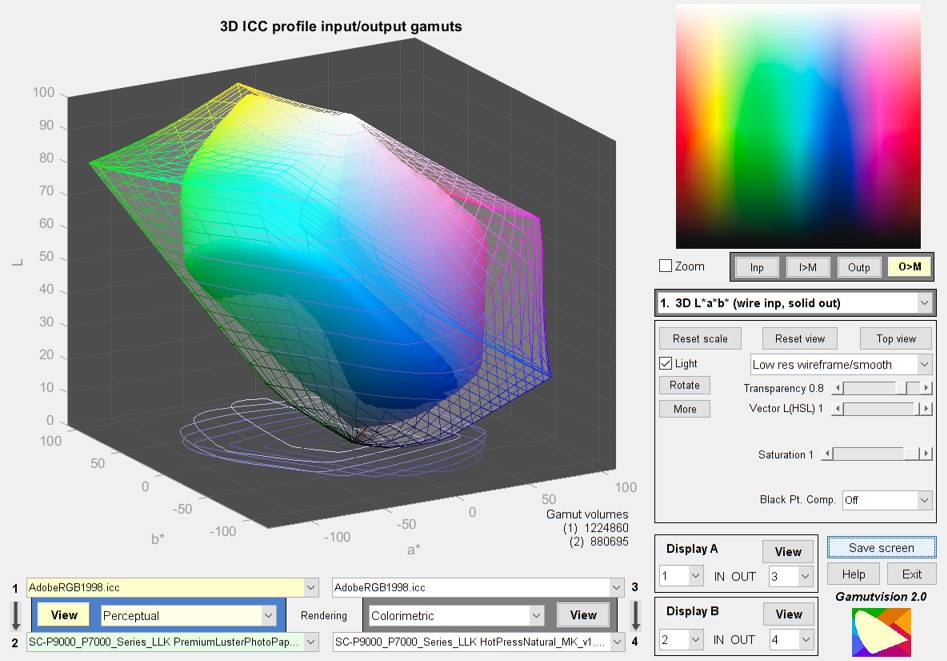 Gamutvision window, showing 3D L*a*b* plot for Adobe RGB to Epson Premium Luster Gamutvision window, showing 3D L*a*b* plot for Adobe RGB to Epson Premium Luster |
|
| The area below the left image is used to select the two input and two output profiles as well as the rendering intents (or none) used to transform the input to the output images. | The right of the Gamutvision window is the plot control area, described below. Saturation = 1 displays the gamut boundary. Lower values display the gamut interior. |
Test pattern (input or output)
This image, located on the upper right of the Gamutvision window, is controlled by selecting one of the four buttons ( , , , ) just below the image. The pattern depends on the display, and may be affected by the Saturation (or Lightness) slider.
| Input image (original) with no mapping. | ||
| Input image mapped to the monitor color space (which defaults to sRGB, but can be set to any monitor profile). | ||
| Output image (original) with no mapping.This image may look strange for printer profiles because it contains the bits sent to the printer, which can have a highly nonlinear relationship to the printed image. | ||
| Output image mapped to the monitor color space (the default). |
Display options area The contents changes for different displays. Details in Displays.
|
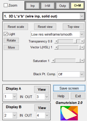 |
Table of Gamutvision displays
This table contains a brief summary of displays. Detailed descriptions can be found in Using Gamutvision Part 2: Displays.
| Display | Display | ||
| 3D L*a*b* (wire input, solid output) (S ≤ 1) A 3D plot in L*a*b* space showing the input gamut as a wire frame and the output gamut as a solid. May be zoomed or rotated (manually or automatically). Vectors and gamut volumes can be displayed. Lighting can be turned on to highlight the gamut surface. S has a default value of 1, but can be set to any value between 0 and 1. |
 |
2D a*b* Gamut (S = 1) 2D Gamut map on the a*b* plane. Shows the input and output gamut for the S=1 (maximum saturation) pattern for L = [0.1, 0.3, 0.5, 0.7, 0.9]. |
 |
| 3D L*a*b* Reversed (wire output) (S ≤ 1) | |||
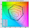
| 2D a*b* Saturation (L(HSL) constant) Shows the input and output gamut response for saturation levels S = [0, 0.2, 0.4, 0.6, 0.8, 1] for fixed values of L(HSL). L has a default value of 0.5 (where colors are the most saturated), but can be set to any value between 0.05 and 0.95. This is an excellent representation of a printer’s color response. |
 |
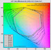
2D a*b* Color difference (L(HSL) constant) Shows the perceptual difference between the input and output gamuts at saturation levels S = [0, 0.2, 0.4, 0.6, 0.8, 1] using fixed values of L(HSL) between 0.05 and 0.95 (default = 0.5). Metrics include ΔE*ab, ΔC*ab, ΔE*94, ΔC*94, ΔE*CMC, ΔC*CMC, ΔL*, ΔChroma, ΔHue angle, and Δ|Hue distance|. |
 |
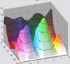
| 3D HL Color difference (S ≤ 1) Detailed 3D or 2D plots of the perceptual differences between the input and output gamut boundaries (saturation S = 1), with the option of reducing S to display the interior of the gamut volume. Metrics include ΔE*ab, ΔC*ab, ΔE*94, ΔC*94, ΔE*CMC, ΔC*CMC, ΔL*, ΔChroma, ΔHue angle, and Δ|Hue distance|. Input and output Lightness (L*) and Chroma (c*) can also be displayed. |
 |
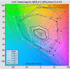
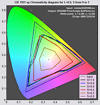
xy Chromaticity (L(HSL)=0.5) CIE 1931 xy Chromaticity pattern. L(HSL)=0.5 pattern. Shown with gamuts for S = [0, 0.2, 0.4, 0.6, 0.8, 1]. Familiar but not perceptually uniform: greens are greatly exaggerated. |
 |
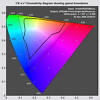
| u’v’ Chromaticity (L(HSL)=0.5) CIE 1976 y=u’v’ Chromaticity pattern. L(HSL)=0.5 pattern. More perceptually uniform than the CIE 1931 xy diagram, but still not perfect. |
 |
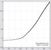
Black & White density response Grayscale density response, typically Density (-log10(reflectance)) vs. log10 pixel level. The digital counterpart of traditional density curves. Uses the Grayscale pattern. The output L*, c* vs. input L* plot displays deviation from neutrality. The best display for observing the effects of Black point compensation. |
 |
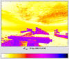
| Read image for analysis (external image file) Images (2D pseudocolor 3D L*a*b* vector plot) representing the perceptual differences between input and output colors— typically between an image and printed output. Same metrics as the color difference plots. Uses the contents of an image file (not a built-in pattern). |
 |
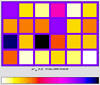
X-Rite/Calibrite ColorChecker® Analyzes a simulated ColorChecker using the same options as Read image for analysis, i.e., 2D pseudocolor analysis or 3D L*a*b* vector analysis. |
 |
| Reference file Convert ideal L*a*b* reference files from Imatest Test Charts to accurate reference files. |
Profile Info Text from the header, including profile type, profile connection space, etc. |
|
(Right) An early colourization fiasco, doomed when the colourists failed to agree on the rendering intent for mapping [255, 255, 255] to [255, 0, 0]. They never even got to the colorimetric meaning of these numbers, From our colour space-case file. |
 |
Menu settings
The menu bar at the top of the Gamutvision window contains three pulldown menus labeled .
File
Save screen Displays and optionally saves a snapshot of the Gamutvision screen as a PNG image file. It also allows you to immediately view the snapshot so it can be used a reference for comparing with other results.
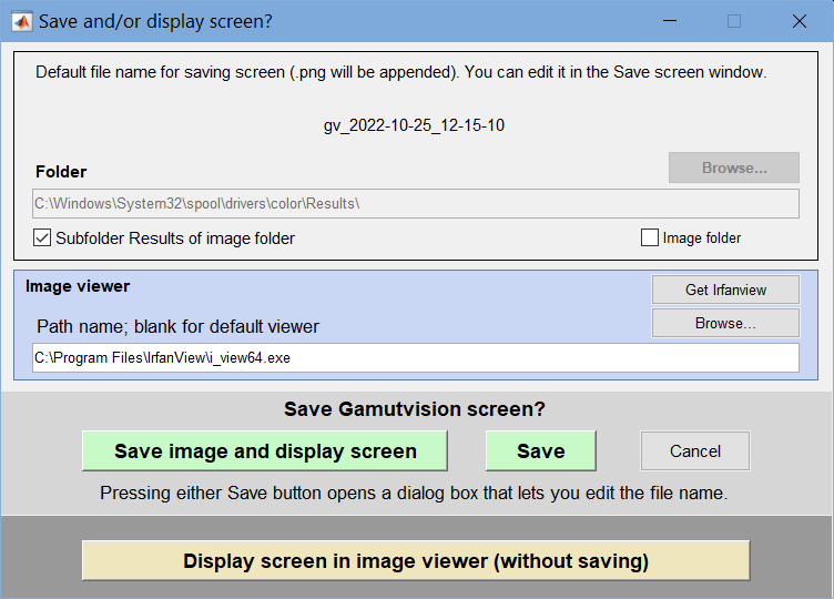
File name and Folder at the top of the window set the location of the file to save.
When you check the Open window in an image viewer… box, the current screen will be opened either the system default viewer (if the box under Image viewer is blank) or a viewer/editor of your choice (if the box contains the path name to the viewer/editor). I recommend using Irfanview, which is fast, compact, free, and supports an amazing number of image file formats. Its normal location in English language installations is C:\Program Files\IrfanView\i_view32.exe.
- Close Closes Gamutvision. Same effect as pressing or clicking on the upper right.
Settings
- ICC Profile folder Select the folder where ICC profiles are kept. Initially set to the system default profile folder (C:\WINDOWS\system32\spool\drivers\color for Windows).
- Monitor profile Select the monitor profile and rendering intent. Defaults to *sRGB (the built-in sRGB profile) and (Relative) Colorimetric intent.
- 3D Plot Select options for the 3D L*a*b* plot. Same as pressing in the 3D L*a*b* plot Display options.
- Small fonts/Normal fonts/Large fonts Select font size. May help appearance for very large screen resolutions or when DPI is set to Large size in the Main tab of the Advanced Display Settings. Change the font size if it appears too large or small relative to the other features.
- Reset screen sets the screen to its original position and size.
- Save settings Save the contents of gamutvision.ini, which contains all current Gamutvision settings, in a named file.
- Retrieve settings Retrieve the Gamutvision settings contained in a named file.
 View settings View the contents of gamutvision.ini in the Notepad viewer.
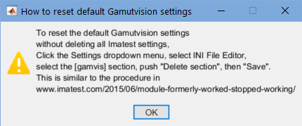
- Default settings Displays a message (shown on the right) indicating how to repair the [gamvis] section of imatest-v2.ini, where a corrupted setting can cause Gamutvision to crash. Follows the procedure in A module that formerly worked has stopped working.
- Save 3D view Save the current 3D view (angle and zoom) in a named (.ini) file. Does not work for 2D views.
- Retrieve 3D view Retrieve a 3D view, previously saved, from a named (.ini) file. Does not work for 2D views.
Display Lets you sent font size (small – XL) or reset the screen (location and size).
Help
- Online Help Open online instructions in a web browser
- About Version and registration information.
- Show welcome text
Gamutvision applications, tips, and techniques are found in the Table of Contents/Site Map on the main Gamutvision page.
Limitations and issues
View scaling. The scaling or appearance of the view may occasionally be incorrect, especially after unusual views or zooms have been applied. The view can be restored by pressing a combination of the , , and buttons.
Embedded ICC profiles. Gamutvision cannot read ICC color profiles embedded in image files. This only affects the Image color difference function. You must enter the appropriate ICC profile.
Device-link profiles. Gamutvision does not currently support device-link profiles. We hope to add that capability in the future. If you try to read a device-link profile, you may get an error that terminates Gamutvision, and this error may repeat when you try to reopen it. If this happens, either (A) delete the [gamvis] section of imatest-v2.ini, following the recommendations in A module that formerly worked has stopped working, or (B) edit imatest-v2.ini (a simple ASCII text file), and remove the line with the offending file name in the [gamvis] section. There is no need to replace it.
OpenGL. The 3D L*a*b* display uses the OpenGL renderer. This may have caused instability on some computers with older versions of MATLAB. If you have issues, for example with Wire frame views, try changing the setting.
Printing. The Gamutvision window cannot be printed directly due to compiler limitations. You must print it from an image editor after either (a) saving it and opening it in the editor or (b) copying it to the clipboard using Alt-PrintScreen (in Windows), then pasting it into the image editor. Irfanview is a nice free image viewer that does the job well.
