Although sharpness is an important image quality factor,
a sharper lens is not always better.
A lens can be too sharp for a sensor, resulting in disturbing visual artifacts.
These artifacts, which include “stair-stepping” and moiré patterns (low frequency patterns that can be strongly colored), can appear because digital cameras— and all digitally sampled systems— have a maximum spatial frequency, called the Nyquist frequency, beyond which scene information cannot be correctly reproduced. Any information above the Nyquist frequency that reaches the sensor will be “aliased” to a lower spatial frequency, which can result in the artifacts described below.
Sampling – Nyquist – Aliasing – Color Moiré – The Imatest Educational App – Effects of aliasing on MTF
Slanted-edge limitations – Wedges
Sampling Courtesy Wikipedia
Sampling
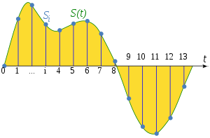
Digital sampling— converting a continuous analog signal into a discrete digital signal— involves two operations.
- Sampling— acquiring the value of the continuous signal at specified intervals.
- Quantization— converting the continuous analog samples into discrete digital samples, for example turning 0-1 volts into digital levels 0-255 (for 8-bit systems). Quantization is not discussed on this page.
The Nyquist sampling theorem
The Nyquist sampling theorem states that if a signal is sampled at a rate dscan and is strictly band-limited at a cutoff frequency fC no higher than dscan / 2, the original analog signal can be exactly reconstructed. The frequency fNyq = dscan / 2 is called the Nyquist frequency. By definition fNyq is always 0.5 cycles/pixel.
The Nyquist frequency can be visualized as the frequency that has two samples per cycle.
Lower frequencies (more than two samples per cycle) can be reproduced exactly, but higher frequencies cannot.
The (geeky) math for reconstructing the original signal is in Wikipedia. It involves a sinc (sin(x)/x) function, which is generally not used in digital imaging.
The first sensor null (the frequency where a complete cycle of the signal covers one sample, hence must be zero regardless of phase) is twice the Nyquist frequency. This means that image sensors can have large average sensitivity (the average of all sampling phases) at and above the Nyquist frequency, which can cause significant visible artifacts.
Aliasing
Signal energy above fN is aliased— it appears as artificially low frequency signals in repetitive patterns, typically visible as moiré patterns. In non-repetitive patterns aliasing appears as jagged diagonal lines— “jaggies” or “stair-stepping” (a less severe form of image degradation). The figure below illustrates how response above the Nyquist frequency leads to aliasing.
| Signal (3fNyq /2) | ||||||||||||||||||||||||
| Sensor pixels |
1
|
2
|
3
|
4
|
5
|
6
|
7
|
8
|
||||||||||||||||
| Response ( fNyq /2) |
In this simplified example, sensor pixels are shown as alternating pink and cyan zones in the middle row. By definition the Nyquist frequency is 1 cycle in 2 pixels = 0.5 cycles/pixel. The signal (top row; 3 cycles in 4 pixels) is 3/2 the Nyquist frequency, but the sensor response (bottom row) is half the Nyquist frequency (1 cycle in 4 pixels)— the wrong frequency. It is aliased.
Image sensors respond to signals above Nyquist— MTF is nonzero,
but because of aliasing, it is not good response.
|
In digital cameras with Bayer color filter arrays— sensors covered with alternating rows of RGRGRG and GBGBGB filters— the problem is compounded because the spacing between pixels of like color is significantly larger than the spacing between pixels in the final image, especially for the Red and Blue channels, where the Nyquist frequency is half that of the total image. This can result in color moiré, which can be highly visible in repetitive patterns such as fabrics. Demosaicing programs (programs that fill in the missing colors in the raw image) use sophisticated algorithms to infer missing detail in each color from detail in the other colors. These algorithms can have a significant effect on color moiré. |
 Bayer CFA Bayer CFA |
Many digital camera sensors— especially older cameras with interchangeable lenses— have anti-aliasing or optical lowpass filters (OLPFs) to reduce response above Nyquist. Anti-aliasing filters blur the image slightly, i.e., they reduce resolution. Sharp cutoff filters don’t exist in optics as they do in electronics, so some residual aliasing remains, especially with very sharp lenses. The design of anti-aliasing filters involves a tradeoff between sharpness and aliasing (with cost thrown in).
|
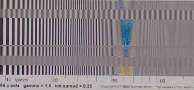
Extreme aliasing. The long-discontinued 14-megapixel Kodak DCS 14n (the first full-frame 24x36mm DSLR), had no anti-aliasing filter. With sharp lenses, MTF response extended well beyond the Nyquist frequency. The 14n behaved very badly in the vicinity of Nyquist (63 lp/mm), as shown in this MTF test chart image, supplied by Sergio Lovisolo. This color moiré is about as bad as it gets. This camera was sold into the wedding photography market, where moiré on wedding gowns made for some very unhappy customers: bad for the photographer and bad for Kodak. |
 |
Recent DSLRs with 30+ megapixels (for full-frame sensors) have pixels that are small enough do that moiré is rarely troublesome (at least on non-repetitive patterns). These cameras don’t have anti-aliasing filters, resulting in a larger image quality improvement than might be expected from the increased pixel count alone.
The Foveon sensor used in Sigma DSLRs is sensitive to all three colors at each pixel site. It also has no anti-aliasing filter, so it can have high MTF at Nyquist, but aliasing is less visible because it is monochrome, not color.
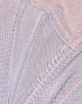
Color moiréColor moiré is artificial color banding that can appear in images with repetitive patterns of high spatial frequencies, like fabrics or picket fences. The example on the right is a detail of a shirt captured by the Canon Rebel XT (an older APS-C DSLR with relatively large pixels) with its excellent kit lens. Color moiré is the result of aliasing in image sensors that employ Bayer color filter arrays, as explained below. Key points:
|
Color moire example: Fabric taken with |
The imatest Educational App
Imatest includes a set of Educational apps that let you visualize the Sampling theorem as well as several other concepts such as MTF and sharpening.
To open the Educational App,
- Click on Help (dropdown menu), then Educational Apps in the Imatest main window, or
- Click on the Help tab in the box on the right, then select Educational Apps.
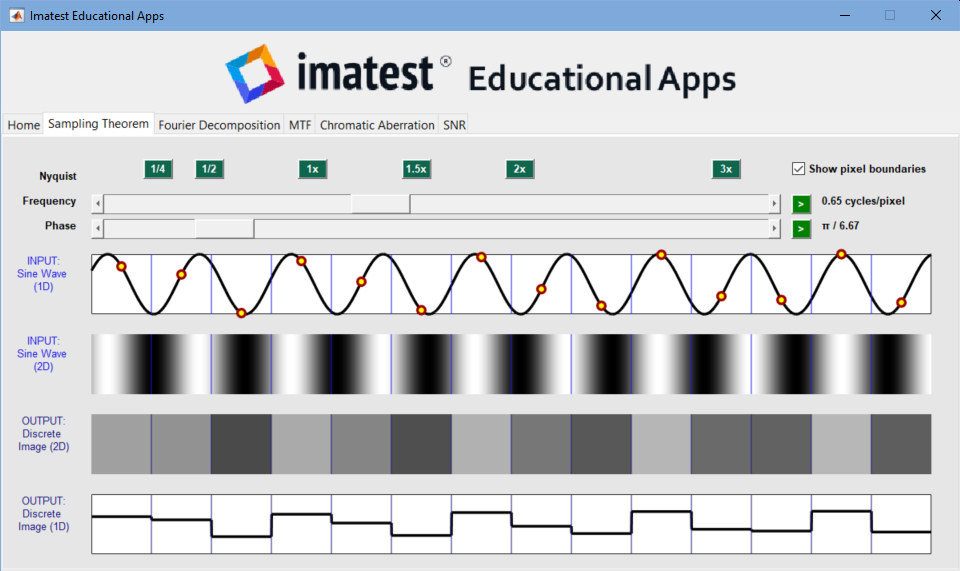 The Imatest Educational app, illustrating the Sampling theorem.
You can adjust the Frequency and Phase with sliders.
By adjusting Frequency you can see how aliasing (output signal at a lower frequency than the input signal) starts at Frequency = 1x (0.5 cycles/pixel). Adjusting Phase with Frequency set to 1x illustrates the phase sensitivity of the output, which varies from maximum to zero amplitude.
The Educational App is helpful for visualizing the sampling theorem and aliasing. Try it.
Effects of Aliasing on MTF measurementsStrong aliasing means that the lens has significant response well beyond maximum frequency where data can be reconstructed— the Nyquist frequency (fNyq = 0.5 C/P). It causes artifacts such as stair-stepping and moiré fringing, which corresponds to the boosted MTF at f > fNyq. The extreme artifacts caused by extreme aliasing can make measured results invalid — they have no real meaning. Aliasing can have significant effects on performance when MTF at fNyq is larger than about 0.20 or 0.25. The image on the right is well beyond that. It has both extreme sharpening (standard sharpening with radius = 2 — stronger than any of the examples on the Sharpening page) as well as extreme aliasing. As a result, measured MTF summary metrics are quite meaningless. A few comments.
|
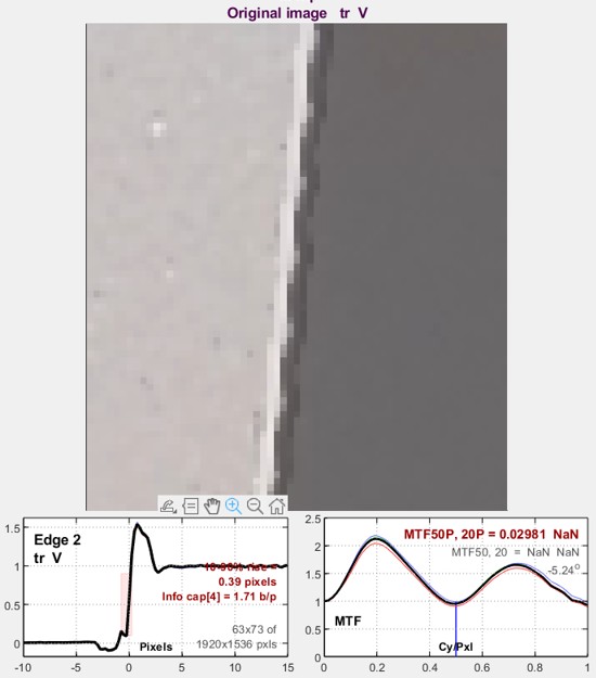 MTF for an edge with extreme aliasing (visible as “stair-stepping”) and sharpening (visible as a “halo” near the edge) The cyclic MTF response is explained in Sharpening examples. MTF for an edge with extreme aliasing (visible as “stair-stepping”) and sharpening (visible as a “halo” near the edge) The cyclic MTF response is explained in Sharpening examples. |
Slanted-edge MTF— why it doesn’t tell the whole story
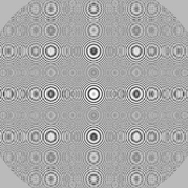
The original zone plate pattern consists only of concentric circles. Everything else is Moiré, resulting from sampling the original pattern without anti-aliasing (lowpass filtering).
Thanks to the ISO 12233 binning algorithm, slanted-edges can measure system response above the Nyquist frequency (fNyq = 0.5 cycles per pixel). As we have shown, response above the fNyq can lead to aliasing artifacts such as moiré, but there are some limitations to MTF measurements— especially with the slanted-edge MTF measurement, which is Imatest’s preferred method (in most instances) because of its speed and efficient use of space.
The limitations are
- The standard output (processed; not raw) of most consumer cameras is sharpened, which significantly boosts response at high spatial frequencies. The amount and the range of frequencies where response is boosted depends on the sharpening amount, radius, and algorithm. Since sharpening has little effect on aliasing artifacts (which depend on the spatial frequency spectrum of the light reaching the sensor and the demosaicing algorithm), the response of sharpened images can be quite misleading.
- Color moiré is difficult to see on slanted edges. It is actually present in the form of colored pixels close to the edge, but it’s difficult to see in non-repetitive patterns.
- Moiré is much more visible on
- hyperbolic wedges (a converging bar pattern),
- Siemens stars, which unfortunately have a very limited area of high spatial frequencies, and
- Log Frequency-Contrast, where moiré is quite visible but difficult to measure quantitatively.
Moiré is exceptionally visible on zone plate patterns (a kind of worst case pattern that can be created with the Imatest Test Charts module), but the zone plate is not suited for quantitative measurements.
Because it is difficult to correlate MTF measurements with visible aliasing, strong MTF response above Nyquist should be regarded only as a warning that aliasing might be an issue and hence needs to be explored further. It is not a definite indicator of aliasing. Imatest techniques for directly measuring the effects of aliasing are listed below.
Wedges
Wedges, which are analyzed by Imatest’s Wedge and eSFR ISO modules, provide the best visual indication as well as measurement of aliasing. Wedges can be used to calculate
- MTF (with limited accuracy because of high contrast and because subpixel variations of sampling phase can cause significant variation of MTF).
- the onset of aliasing (also called “vanishing resolution”; the spatial frequency where the bar count starts decreasing).
- the effects of aliasing, especially color moiré.
Wedges can be manually selected in the old ISO 12233:2000 chart with the Wedge module, which we don’t recommend because it’s inconvenient. (and the old chart is also not recommended by the current ISO 12233:2014+ standard). We strongly recommend using the eSFR ISO chart and module, which is compliant with the current standard and automatically detects wedges and other features. It measures a great many image quality factors (MTF, Lateral Chromatic Aberration, color, tonal response, noise, Signal-to-Noise Ratio, and more) in addition to color aliasing. Wedge moiré plots are identical in the Wedge and eSFR ISO modules. We illustrate eSFR ISO results below.
The Wedge moiré plot
The Wedge moiré plot below shows the mean CIELAB chroma (\(C^* = \sqrt{a^{*2} + b^{*2}} \) ) measured inside the wedge as a function of spatial frequency. Several other color aliasing-related metrics are listed in the table below.
To get the plot below, acquire an eSFR ISO chart image,then run eSFR ISO Setup, following the instructions here. eSFR ISO can also be run in batch-capable Auto mode. Under Display, select 18. Wedge moiré.
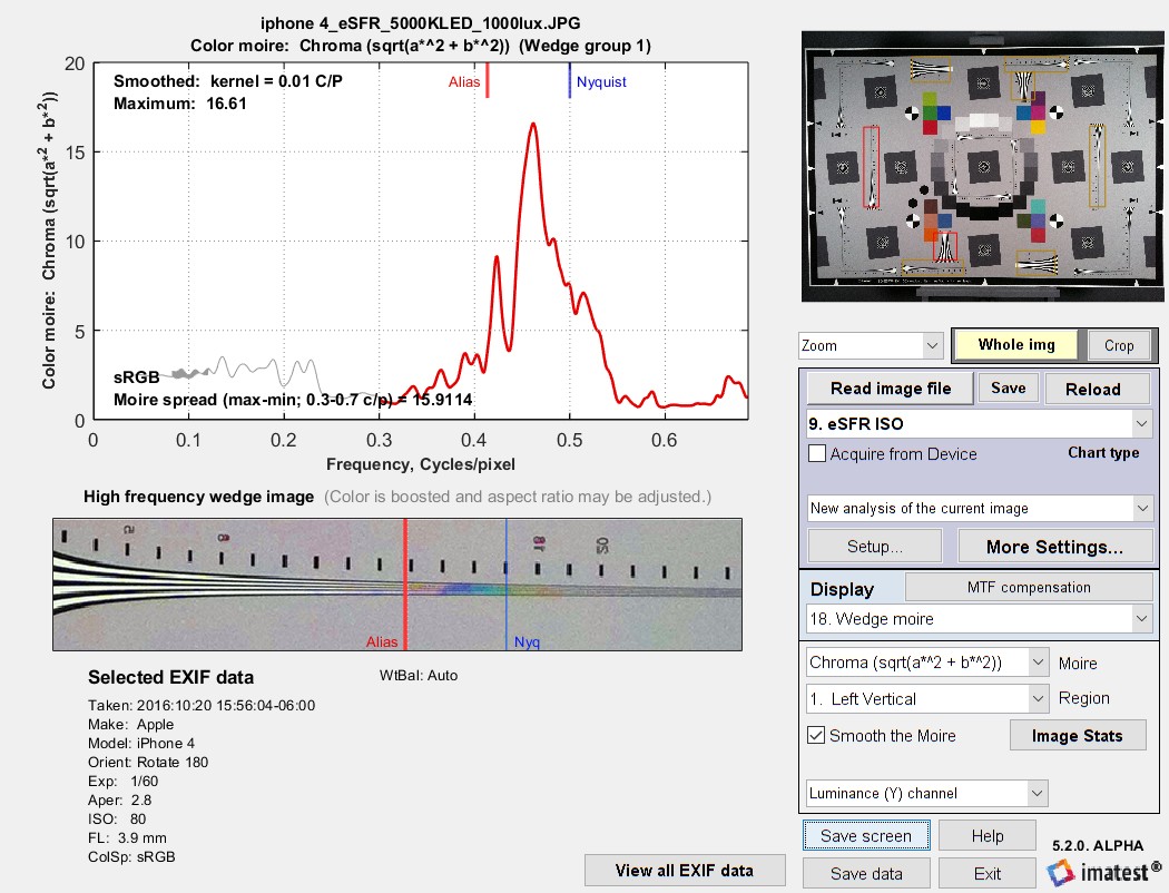 Color aliasing (CIELAB Chroma) for an older iPhone with significant color aliasing.
Chroma has been boosted in the image.
The curve in the plot is the mean of the selected metric (\(C^* = \sqrt{a^{*2} + b^{*2}} \) in this case), taken inside the wedge as illustrated below.
 Segment of wedge (enlarged from above chroma-boosted image). Spatial frequency increases from left to right.
Metric for each frequency is obtained by averaging the parameter (example: |R-B|) inside the wedge.
The table below lists the available metrics, which are selected in the Moiré dropdown menu on the right side of the image below Display. Only three of the metrics are recommended: the others are informative or experimental. The maximum value of each metric is displayed in the upper left of the plot (shown above). The maximum values for all the metrics can be saved in JSON and CSV results files. Here is a list of the metrics, emphasizing the recommended metrics.
| mean(|R-B|) | This is a good metric since the Red and Blue channels are most affected by color aliasing. |
| mean(|R-B|) / mean(R,B) | This is slightly more stable since it’s normalized to the mean value of R and B. |
| mean(|R-G|) | These may be interesting to examine, but they tend to be less sensitive than R-B metrics because the green (G) channel has a higher Nyquist frequency. |
| mean(|R-G|) / mean(R,G) | |
| mean(|G-B|) | |
| mean(|G-B|) / mean(G,B) | |
| S(HSL) | These Saturation metrics are not recommended because they can have large values at low levels (L or S), hence can be misleading. They may not be kept. |
| S(HSV) | |
| Chroma \(C^* = \sqrt{a^{*2} + b^{*2}} \) | CIELAB Chroma, \(C^* = \sqrt{a^{*2} + b^{*2}} \) This is the primary (recommended) color aliasing metric. |
Color aliasing metric
The color aliasing metric is new in Imatest 5.1.12, released in October 2018. Prior to this release the color metrics did not correlate well with image appearance. The metric to display is selected in the Moiré dropdown menu, below Display.
Each wedge region is white-balanced prior to calculating the color aliasing metrics. The metrics are calculated inside the wedge. Smoothing (with a kernel of width 0.01 Cycles/Pixel) is recommended for consistent results. The color moiré metric is selected in the Moiré dropdown menu. Our primary recommended metric is Chroma (sqrt(a*^2 + b*^2)). This is the mean of the CIELAB chroma, C = sqrt(a*2 + b*2). Other useful color aliasing metrics are mean(|R-B|) and mean(|R-B|) / mean(R,B). |R-B| is useful because Red and Blue are more sensitive to aliasing then Green.
Clicking Save data (or running eSFR ISO setup with the appropriate boxes checked) saves data to CSV and JSON files. Here is a sample of JSON output for the color aliasing summary metrics (the maximum value for each metric shown in the above table). Recommended metrics are shown in boldface.
“color_aliasing_max_mean_R_minus_B”: [0.1327,0.1088,0.07527,0.07033],
“color_aliasing_max_mean_R_minus_B_normalized”: [0.391,0.2999,0.4362,0.3822],
“color_aliasing_max_mean_R_minus_G”: [0.09607,0.02452,0.08199,0.07815],
“color_aliasing_max_mean_R_minus_G_normalized”: [0.328,0.05977,0.4449,0.3945],
“color_aliasing_max_mean_G_minus_B”: [0.1041,0.1088,0.06335,0.03999],
“color_aliasing_max_mean_G_minus_B_normalized”: [0.2701,0.2991,0.2851,0.1786],
“color_aliasing_max_mean_S_HSL”: [0.6033,0.9159,0.4902,0.5427],
“color_aliasing_max_mean_S_HSV”: [0.3227,0.2781,0.4083,0.3311],
“color_aliasing_max_mean_CIELAB_chroma”: [16.61,16.48,10.69,11.19],