Introduction to Acutance and SQF
Acutance and Subjective Quality Factor (SQF) are measures of perceived print or display sharpness. SQF was used for years in the photographic industry but has remained unfamiliar to most photographers. Acutance is a relatively new measurement from the IEEE Camera Phone Image Quality (CPIQ) group. Both are metrics which incorporate the effects of
- The imaging system: The Modulation Transfer Function (MTF) of the camera as a measurement of its intrinsic sharpness.
- The viewer: The human eye’s sensitivity to each spatial frequency modeled with a Contrast Sensitivity Function (CSF).
- The viewing conditions: The image display height and viewer-to-display distance which describe how the image display fills the human eye.
These metrics are used to describe perceived sharpness of the final product image as viewed by a human, not just the intrinsic properties of the camera. This helps describe common accounts such as “This image looks sharp when I look at it on a mobile phone, but when I zoom in on a computer screen it doesn’t look sharp at all.”
Because of the CPIQ standardization work, which includes correlation of acutance numbers to perceptual quality loss units of Just Noticeable Differences (JNDs) we generally recommend acutance over SQF. In later sections of this page we may refer only to acutance for brevity, but the description is assumed to apply to SQF as well.
History
SQF was introduced in the paper, “An optical merit function (SQF), which correlates with subjective image judgments ,” by E. M. (Ed) Granger and K. N. Cupery of Eastman Kodak, published in Photographic Science and Engineering, Vol. 16, no. 3, May-June 1973, pp. 221-230. (If you do an Internet search, note that Granger’s name is often misspelled Grainger.) It was used by Kodak and Polaroid for product development and is used by Popular Photography for lens tests. This technical paper verified its correlation with viewer preference. But SQF is rarely mentioned on photography websites with the notable exception of Bob Atkins‘ excellent description, which includes an explanation of Pop Photo’s methods.
Acutance is a perceptual measurement that is closely related to SQF, but differs in the details of the equation. It is defined in the IEEE CPIQ (Camera Phone Image Quality) Phase 2 specification, but this document gives little indication of how it should be displayed. Imatest displays it in the same way as SQF.
Acutance and SQF can be measured in many of Imatest’s sharpness modules: SFR, SFRplus, Star, Random/Dead Leaves, SFRreg, Checkerboard, and eSFR ISO.
Acutance Measurement Options
Acutance or SQF can be measured in Imatest SFR, SFRplus, Star, Random/Dead Leaves, SFRreg, Checkerboard, and eSFR ISO You need to check the Acutance Analysis checkbox in the Settings box (if its present). Settings will be saved for subsequent runs.
Clicking on the button in the Settings window of one of the above modules will open the window for choosing your viewing condition and calculation options.
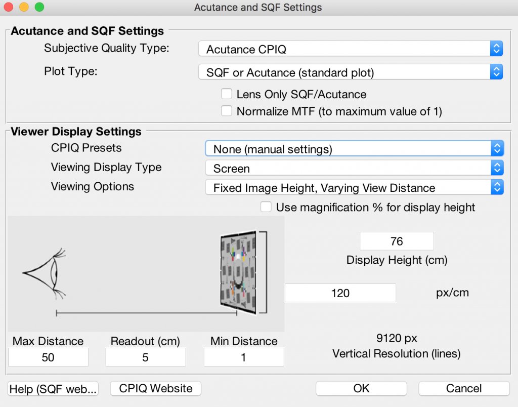
Acutance Options Window
Acutance and SQF Settings
This panel contains calculation and output plot options which are independent of the observer view conditions.
Subjective Quality Type
Choice of which integral and which definition of CSF is used in the calculation, those defined by CPIQ for acutance or those which define SQF. (See green boxes below for details.)
Plot Type
Choice of which quantity is plotted as an output- the Acutance/SQF value itself (which is an objective metric) or the perceptual loss value associated with that value (a subjective metric) in JNDs. If JND plotting is selected, the Subjective Quality Type is forced to be “Acutance CPIQ” since that is the quantity which has the objective-subjective mapping defined.
Lens Only Checkbox
Ignore the contribution of the display medium (print or monitor) on the acutance calculation. When checked, outputs assume a perfect display medium with flat SFR and do not account for a finite number of dots/pixels, effectively making the acutance calculation dependent on the “lens only” and not the final display. (Note that since acutance is derived from MTF and Imatest can only measure MTF from a whole system- lens, sensor, and processing- that it is not actually lens only.)
Normalize MTF
Re-scale the MTF curve which the Acutance is derived from so that its maximum value is 1.
Generally speaking, the maximum of the MTF curve should already be 1 per definition of MTF. However, due to sharpening the MTF curve may sometimes have a peak greater than 1. Selecting this option rescales the MTF curve in such a case.
Viewer Display Settings
This panel comprises options to define the view conditions of an image taken with this device being viewed by an observer. Typically this defines a display size and display distance-from-observer which are used to map device MTF in cy/px to angular MTF in the observer’s eye in cy/deg. It also defines the nature of the display and its resolution, which are critical for determining any resizing that would happen to produce the image on the display.
CPIQ Presets
The CPIQ standard defines five standard view conditions which cover a number of common use cases- Small Print, Large Print, Computer Monitor at 100%, 4.5″ Cell Phone, 30″ 4k TV.
Selecting one of these sets the rest of the options automatically, making the use of this option a good starting point for new users. If “None (manual settings)” is used in this option, the following settings may be set to describe custom view conditions.
Viewing Display Type
Selection between Screen, Print, or Ideal display types. Per the CPIQ standard, the display type determines the MTF of the medium which the image is shown on. Selection of “Ideal” implies the display medium introduces no MTF of its own.
Viewing Options
Determines the independent variable (i.e., x-axis) used to produce a plot of acutance as it changes with respect to the choice. Depending on which of these you choose, the display below will provide different sets of data entry options.
Fixed View Distance, Varying Display Height
The user selects a minimum and maximum display size (in cm) to plot acutance at while the view distance is held at a single value. An additional single height value can be identified as a readout value for easy data output querying.
The x-axis of the output plot will be Display Height over the defined range.
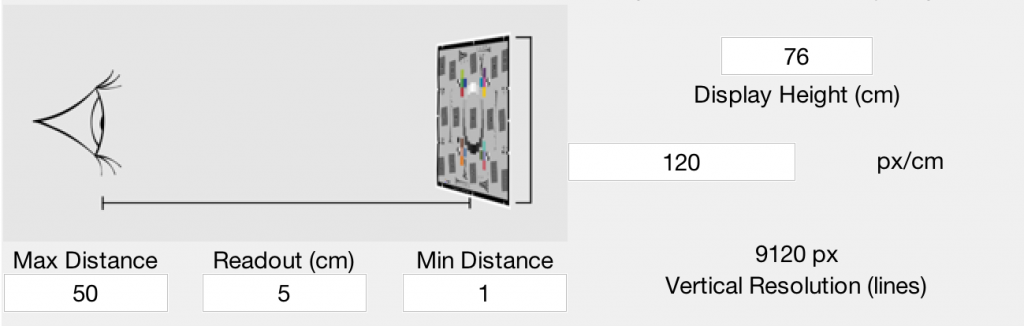
Fixed Display Height, Varying View Distance
The user selects a minimum and maximum viewing distance (in cm) to plot acutance at while the display size is held at a single value. An additional single distance value can be identified as a readout value for easy data output querying.
The x-axis of the output plot will be Viewing Distance over the defined range.
Use magnification % for display height
When checked, the entry boxes for display height are in units of “% magnification of input image” instead of cm.
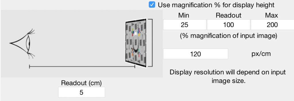
This usage implies that the display size scales appropriately to be the number of rows of the image divided by the dots/cm or px/cm of the display times the magnification. Since the display is obviously not changing its size when data scaling is happening, the display can instead be thought of as a “window” into a display that theoretically was that size.
Example: The CPIQ preset of “Computer monitor viewed at 100%” makes use of this option and implies that the image is viewed on the screen at a scaling such that one pixel in the image becomes one pixel on the screen, rather than being upsized or downsize.
px/cm
The pixels per cm of the display (or dots per cm, for a print) on which the image is assumed to be viewed.
This value is critical to indicate if the display has a smaller resolution than the camera producing the images to be viewed. If so, the images would need to be downsized prior to displaying (unless viewed at, e.g., 100% zoom as in the above example) which changes the spatial frequency content. Imatest models this to a first order with an ideal low-pass filter applied to the imaging system’s measured MTF prior to conversion to angular frequencies.
Acutance and MTF
The following table compares MTF and acutance. In essence, MTF is a measurement of device or system sharpness; acutance and SQF are measurements of perceptual print or diaplay sharpness, derived from MTF, the contrast sensitivity function (CSF) of the human visual system, and viewing angle (based on an assumption about the relationship between print height and viewing distance).
| MTF (Modulation Transfer Function) | Acutance or SQF (Subjective Quality Factor) |
| Measures image contrast as a function of spatial frequency. Describes device or system sharpness. Indirectly related to perceived image sharpness in a print or display. | Measures perceived sharpness as a function of print or display height and viewing distance. Describes viewer experience. Requires an assumption about viewing distance (can be constant or proportional to the square root or cube root of print height). |
| Omits viewing distance and the human visual system. | Includes the effects of viewing distance and the human visual system. |
| Abstract: Plots of MTF (contrast) vs. spatial frequency require technical skill to interpret. | Concrete: Plots of SQF (perceived sharpness) vs. print height require little interpretation. SQF has the same subjective meaning regardless of print size. It can be used to precisely answer questions like, “How much larger can I print with a 12.8 Megapixel full-frame DSLR than with an 8.3 Megapixel APS-C DSLR?” |
| 1.0 at low spatial frequencies. Decreases at high spatial frequencies, but may peak at intermediate frequencies due to sharpening. A peak over 1.4 indicates oversharpening, which can result un unpleasant “halos” at edges, especially for large print sizes. | 100 (%) for small print heights. Decreases for large print heights, but may increase at intermediate print heights due to sharpening. A peak value over about 105% may indicate oversharpening (and over 108% definitely indicates oversharpening). In such cases you should examine the MTF plot and edge profile. |
| The frequency where it drops by half (MTF50) is a reasonable indicator of relative perceived sharpness, but requires interpretation and is not as precise as SQF. | An SQF difference of 5 corresponds to a perceptible change in in sharpness— somewhat more than one “Just Noticeable Difference” (JND). SQF can be used as the basis of a ranking system. JND for acutance is displayed by Imatest. It is described below. |
| Familiar to imaging scientists Gradually becoming familiar to a wider public, though vanishing resolution is still better known. | SQF is unfamiliar in the imaging industry. It was used internally in Kodak and Polaroid, but difficult to measure prior to the advent of digital imaging. Acutance is a relatively new measurement that is becoming familiar thanks to the IEEE CPIQ group. |
| All the measurements (MTF, SQF, and acutance) are strongly affected by sharpening, which is routinely performed to improve perceived sharpness, hence SQF would be expected to increase. | |
Here is a sample result.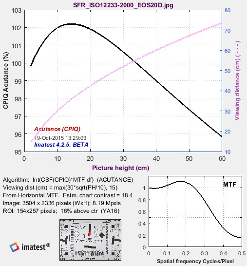
Acutance, based on the assumption that viewing distance = square root of image height.
The solid black line in the top plot shows acutance for print heights from 2 to 60 cm (~2 to 24 inches), assuming viewing distance (cm) = 30 √(picture height/10), which is in the ballpark for gallery viewing conditions. Acutance goes over 100 because the image has a modest MTF peak from sharpening. The top plot also shows viewing distance ( – – – ). The plot on the lower right is the MTF, which is displayed in the main SFR/MTF figure, but repeated here to make this figure self-contained. The lower middle contains a thumbnail of the image showing the selected ROI in red. The text on the left contains calculation details and image properties.
What do the acutance and SQF numbers mean?
SQF— Ed Granger developed SQF to be linearly proportional to perceived sharpness. A change in SQF of 5 corresponds to a perceptible change in sharpness— somewhat more than one “Just Noticeable Difference” (JND). Since we do not have our own database of SQF impressions we’ll draw on the experience of others.
Popular Photography has been using SQF for testing lenses for years. They’ve developed the only generally-available SQF ranking system. Their scale isn’t quite linear. {C, C+} takes up 20 SQF units; twice as many as {A, A+}, {B, B+}, or D. But it seems to be a good starting point for interpreting the numbers.
| A+ | A | B+ | B | C+ | C | D | F |
| 94-100 | 89-94 | 84-89 | 79-84 | 69-79 | 59-69 | 49-59 | Under 49 |
We encourage readers to examine Popular Photography‘s lens test results and to search its site for SQF. Imatest results should correlate with Pop Photo‘s results, but there are a few significant differences.
- Pop Photo measures SQF for lenses alone, while Imatest measures SQF for the entire imaging system. This means that Imatest results are sensitive to signal processing (sharpening and noise reduction; often applied nonlinearly) in the camera and RAW converter. This makes is difficult to compare lenses from measurements taken on different cameras. On the other hand, it means that you know what your camera/lens combination can achieve, and it’s excellent for comparing lenses measured on one camera type (with consistent settings).
- Pop Photo‘s algorithm for calculating SQF (the SQF equation and the viewing distance assumption; both discussed below) is not known.
Quality as a function of SQF
The scale on the right was developed by Bror Hultgren, based on extensive category scaling tests. According to Bror, the perceived quality level depends on the set of test images (particularly how bad the worst of them is) as well as the task (e.g., a group of cameraphone users would rank images differently from a group of art gallery curators), but the relationships between categories remains relatively stable. These levels are comparable to Popular Photography’s scale.
Additional considerations in interpreting SQF:
- SQF has the same interpretation regardless of print size. That means a print with SQF = 92 would have the same quality “feel” for a 4x6 print as for a 24x36 inch print. This is in contrast to MTF measurements, where MTF measured at the print surface is interpreted differently for different sizes of prints: you tend to accept lower MTF for larger prints because you view them from larger distances (though the relationship, described here, is far from linear). Viewing distance is built into SQF.
- The SQF calculation omits printer sharpness (for now). It assumes that modern high quality inkjet printers can print as sharp as the unassisted eye can see at normal viewing distances— a fairly safe assumption for large prints (= 20 cm high).
Acutance— The CPIQ document defines an “objective metric” (OM = 0.8851 – acutance for acutance = 0.8851; OM = 0 otherwise) that increases with increasing blur. It claims that perceived quality does not improve for acutance greater than 0.8851. The result of a rather complicated equation shows that a change in OM of 0.02 (2%) corresponds roughly to 1 JND.
Acutance and SQF equations
Following the convention elsewhere in the Imatest site, we put the math in green boxes, which can be skipped by non-technical readers. The acutance equation is shown first- SQF is primarily of historical interest.
|
\(\displaystyle \text{Acutance} = \frac{\int_0^\infty SFR_L (v) CSF(v) dv}{ \int_0^\infty CSF(v) dv}\) where \(\displaystyle CSF_L(v) = \frac{av^c e^{-bv}}{K} \) where a = 75, b = 0.2, c = 0.8, and K = 34.05, Note that this value of CSF peaks around 4 cycles/degree, much lower than the CSF used for SQF. |
|
|
|
The SQF equation The gist of this box is that Granger presented the full equation for calculating SQF in 1972, but he used a simplified approximation for his calculations. Although the exact equation is strongly recommended, Imatest can use the simplified approximation where needed for comparing new and old calculations. In reviewing older publications, you should determine which calculation was used. The exact equation for SQF implied by Granger is, \(\displaystyle SQF = K \int_0^\infty CSF(f) MTF(f) d(\log f) = K \int_0^\infty \frac{CSF(f) MTF(f)}{f} df\) where CSF( f ) is the contrast sensitivity function of the human eye, discussed below; CSF( f ) is close to zero for f > 60 cycles/degree), Since Granger had limited access to sophisticated computers (the average personal computer today has about as much power as the entire Pentagon had in 1972), he used an an approximation for his calculations assuming that CSF( f ) is roughly constant from 3 to 12 cycles/degree. \(\displaystyle SQF = K \int MTF(f) d(\log f) = K \int \frac{MTF(f)}{f} df\) for 3*cpd < f < 12*cpd; 0 otherwise; \(\displaystyle K = \frac{100\%}{\int d (\log f)} = \frac{100\%}{ \int \frac{df}{f}}\) for 3 cpd < f < 12 cpd is the normalization constant. \(\displaystyle K = \frac{100\%}{\log (12) – \log (3)} = 72.1348\%\) Although Imatest offers the option of using this approximation (as a check on older calculations), the exact equation is recommended. The integration limits used by Granger and Cupery were 10 and 40 cycles/mm in the retina of the eye, which translate to 3 and 6 cycles/degree when the eye’s focal length (FL = 17 mm) is considered. f (cycles/degree) = f (cycles/mm) (π FL) / 180. To calculate SQF it is necessary to relate spatial frequency in cycles/degree, which is used for the eye’s response CSF( f ), to spatial frequency in cycles/pixel, which is calculated by Imatest SFR. \(\displaystyle f(\text{cycles/degree}) = \frac{\pi\: n_{PH}\: d\: f(\text{cycles/pixel})}{180\: PH}\) where nPH is the number of vertical pixels (along the Picture Height, assuming landscape orientation), d is the viewing distance Noisy images In images with long transitions (10-90% risetime r1090 over 2 pixels) and high noise, increasing the noise can increase the SQF, unless we take preventative steps. What we do is to recognize that most signal energy is at spatial frequencies below 1/r1090. At frequencies over 1/r1090 we do not allow MTF to increase: MTF( fn ) = min( MTF( fn-1 ), MTF( fn ) ). This has little or no effect on the MTF due to the edge, but prevents noise spikes from unduly increasing SQF. |
Contrast sensitivity function (CSF)
Contrast sensitivity function
The human eye’s contrast sensitivity function (CSF) is limited by the eye’s optical system and cone density at high spatial frequencies and by signal processing in the retina (neuronal interactions; lateral inhibition) at low frequencies. Various studies place the peak response at bright light levels (typical of print viewing conditions) between 6 and 8 cycles per degree (around 4 for the CSF equation used for acutance). We have chosen a formula, described below, that peaks just below 8 cycles/degree.
You may learn something about your own eye’s CSF by viewing the image below at various distances and observing where the pattern appears to vanish. Contrast is proportional to (y/h)2, for image height h. Although the image appears to decrease in contrast linearly from top to bottom, the middle of the chart has 1/4 the contrast as the top.
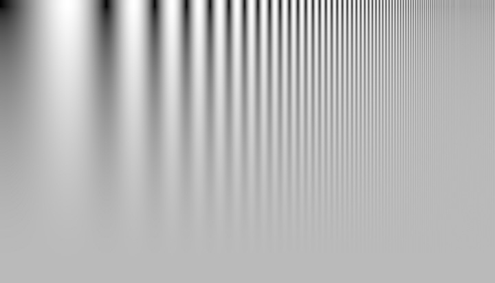
Log frequency-Contrast chart, created by Test Charts.
The Log F-Contrast chart is very similar to the Campbell-Robson CSF (Contrast Sensitivity Function) chart,
which was first published in 1968. The (vertical) contrast variation is quite different for the two charts.
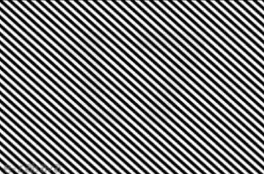
You can learn a lot about CSF by clicking on the slanted-line image on the right to view it full-sized. At normal viewing distance you won’t see the number hidden in it. Move back a few meters and it should become very clear.
What is happening? At normal viewing distances the frequency of the diagonal bars has a high CSF value, while the lower frequency of the hidden number is has a relatively low CSF value When you move back, the CSF of the bars is reduced but the CSF of the hidden number is much higher, making it easy to see.
Click on the image to view full-sized.
Move back several meters to see the hidden number.
|
For SQF, we have chosen a formula that is relatively simple, recent, and provides a good fit to data. The source is J. L. Mannos, D. J. Sakrison, “The Effects of a Visual Fidelity Criterion on the Encoding of Images”, IEEE Transactions on Information Theory, pp. 525-535, Vol. 20, No 4, (1974), cited on this page of Kresimir Matkovic’s 1998 PhD thesis. \(\displaystyle CSF (f) = 2.6 ( 0.0192 + 0.114 f) e^{-{(0.114 f)}^{1.1}}\) The 2.6 multiplier drops out of SQF when the normalization constant K is applied. This equation can be simplified somewhat. \( CSF(f) = (0.0192 + 0.114 f) e^{-0.1254f}\) The preferred SQF equation, \( SQF = K \int CSF(f) MTF(f) d(\log f) = K \int \frac{CSF(f) MTF(f)}{f} df \), blows up when the dc-term (0.0192) is present. Fortunately, as the above plot shows, removing it makes very little difference. The formula used to calculate SQF in the preferred equation is CSF( f ) = 0.114 f exp(-0.1254 f ). |
| More geek stuff (additional equations that have been deprecated) Some additional equations were included in the SQF options for experimental study.They have been deprecated because acutance has become a standard. \(SQF = K \int_0^{\infty}\! CSF(f) MTF(f) \, \mathrm{d} log f \,\, = K \int_0^{\infty}\! (CSF(f) MTF(f))/f \, \mathrm{d} f\) where \( K = \frac{100\%}{\int CSF (f) df} \) or \( K = \frac{100\%}{log (\int CSF(f) df)}\) is the normalization constant. These equations were developed to address concerns about d(log f ) = d f /f , which becomes very large at low spatial frequencies. Integrals containing this term blow up if CSF( f ) contains a dc (constant) term. Fortunately, as noted above, removing the dc term from CSF makes very little difference and works quite well, so we only keep these equations for experimental purposes. Granger used d(log f ) because he noticed that a constant percentage change in MTF corresponded to a just noticeable difference, i.e., the eye responds logarithmically. Equation 1 is linear. Equation 2 is logarithmic, but presents some scaling problems: What to do about log(1) = 0? Should we use log10 (comparable to density measurements), log2 (comparable to exposure value or f-stop measurements), or loge (in accordance with Boulder, Colorado community standards, where only organic, natural logarithms are employed)? We’ve chosen not to pursue these equations. |
Links
Bob Atkins‘ excellent introduction to MTF and SQF is highly recommended.
Popular Photography has been using SQF for testing lenses for years. Their test results are well worth exploring.
