Analyze the Siemens Star chart
|
New in Imatest 2020.1 (Feb. 2020) Shannon information capacity can be calculated from images of the Siemens star, with much better accuracy than slanted-edges. The old slanted-edge method has been deprecated.
Imatest 5.0:
Imatest 4.0: Automatic region detection is available for a new version of the Star Chart that has registration marks on the sides. See below. |
Introduction – Creating, photographing, running – Output – MTF – MTFnn, MTFnnP
MTF contours – Information capacity – Sine vs. bar – Equations
Introduction
Star Chart, which can be run in the interactive Rescharts interface or as a fixed (batch-capable) module, measures SFR (Spatial Frequency Response); also known as MTF (Modulation Transfer Function) from Siemens star charts, which are included the ISO 12233:2014 standard. It can also measure the information capacity of pixels. Sinusoidally-modulated stars are preferred, but bar (square wave-modulated) Siemens stars can also be analyzed for MTF, with appropriate normalization settings.
A detailed comparison of Siemens Star and slanted-edge MTF results is presented in Slanted-edge versus Siemens Star – A comparison of sensitivity to signal processing. For most sharpness measurements we recommend the slanted-edge, which are accurate, reliable, run fast, and can produce highly detailed maps of sharpness over the image surface. But we strongly support the Siemens Star, which provides information on angular MTF response and is the only pattern other than the slanted-edge that can analyze MTF response above the Nyquist frequency. It also enables noise to be measured in the presence of the signal), which is the basis of the calculation of Shannon information capacity, which is an excellent camera quality metric (figure of merit) that has traditionally been difficult to measure.
Charts with 144, 72, 48, 36, 24, and 16 cycles can be analyzed in 8, 16, or 24 segments around the circle. (ISO 12233 recommends 144 or 72 cycles.) Several options are provided for calculating the value of gamma used to linearize the chart and for the low frequency reference.
Photographing the chart and running the program
Star Chart measures MTF from a star pattern along the radii of a circle for a range of angles (in 8, 16, or 24 segments). Although sinusoidally-modulated patterns are preferred, bar (square wave-modulated) patterns will work with an appropriate normalization setting. This method is more direct than the slanted-edge method, but requires more real estate. Because calculations are performed on circles of known spatial frequencies, the results are more robust against noise than Log Frequency, which also uses a sinusoidally-modulated pattern.
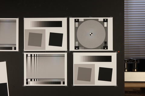 Image with star chart (upper right)
The image above was used to compare Star chart results with Slanted-edge SFR and Log Frequency. It was captured with a Canon EOS-40D camera, 24-70mm f/2.8L lens set at 50mm, f/5.6, ISO 100. It includes Star, Log Frequency-Contrast and slanted-edge charts with high and low contrast (20:1 and 2:1).
We recommend that you purchase test charts from the Imatest Store. You can also create a file with the Imatest Test Charts module that can be printed on a photographic quality inkjet printer. Recommended options are PPI: 720 (Epson inkjets) or 600 (HP or Canon inkjets), Height (cm) (as required), Highlight color: White, Contrast ratio: 50, Type: Sine, Gamma: 2.2, Star pattern bands: 144 or 72 (for high or low resolution cameras, respectively), Chart lightness: Lightest, ISO standard chart: Small (1/20) inner circle (inner circle has 1/20 the diameter of the outer circle). Cheap bond paper and laser printers are strongly discouraged.
|
Number of chart cycles Ideally the maximum spatial frequency (just outside the inner circle) should be around 0.6 to 1.0 cycles/pixel. The diameter of the inner circle di is typically 1/20 times the diameter dP of the circular star pattern, depending on the chart (selectable in Test Charts). The smallest diameter for analysis is 0.056dP or near-zero (for no center circle). For an image of P pixels (width or height) of a star with N cycles, where the pattern circle diameter dP takes up a fraction g of P (dP = gP; di = 0.056 gP ) , the maximum spatial frequency in cycles/pixel is \( f_{max} = \frac{N}{0.056 \pi d_{P}} = \frac{N}{0.056 \pi g P}\) (inner circle 1/20 the diameter of the outer) Example: for a 3000 pixel wide image where the pattern circle dP takes up g = 1/3 (33.33%) of the image and the inner circle has 1/20 the outer diameter, fmax = 0.818 cycles/pixel for a 144-cycle pattern; fmax = 0.414 cycles/pixel for a 72-cycle pattern. The 144-cycle pattern is indicated. 72-cycle patterns are most suitable for low resolution cameras (~2 megapixels or less). |
Mount the chart on a flat dark board— 1/2 inch foam board works well; thinner board warps more easily. Depending on the number of horizontal pixels in the image to be analyzed, the chart should occupy approximately 500-2000 pixels, typically 1/3 to 1/4 of the horizontal frame for high resolution cameras (more of the frame for lower resolution cameras: VGA, etc.). Other charts can be mounted along with it.
Orientation.
The chart itself contains no clear indication of the recommended orientation. We recommend the following orientation (though Imatest will correct for incorrectly oriented charts).
– The pattern should be oriented horizontally, i.e., in landscape orientation (it is slightly wider than high).
– The darkest grayscale patches should be in the lower-right of the image; the lightest should be in the upper-right.
Photograph the chart using glare-free even lighting (±5%, which should be easy to achieve since the chart is relatively small), as described in Building a Low-Cost Test Lab or How to test lenses. Save the image in any one of several high quality formats, but beware of JPEGs with high compression (low quality), unless you are testing for JPEG degradation.
|
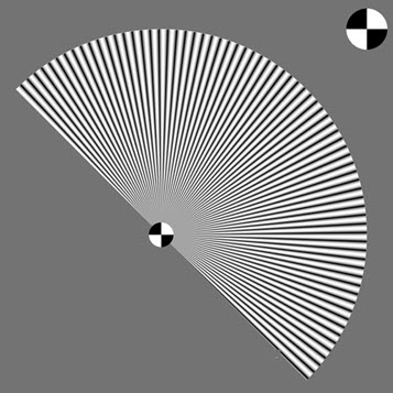
Because resolution varies over the image for most cameras and lenses, the chart should not take up too much of the frame. The active chart height (the Star diameter) should be between about 500 and 2000 pixels, with at least 800 pixels recommended for high resolution cameras. For typical high resolution cameras the active chart height should be no more than about 1/3 to 1/2 of the total image height, i.e., the area of the star pattern should not exceed about 1/8 of the total chart area. This recommendation does not apply to low resolution systems such as VGA, which need at least 300 pixels of active chart height (more if possible). Here is additional information from the page on Shannon Information Capacity. The size of the star in the image should be set so the maximum spatial frequency, corresponding to the minimum radius rmin, is larger than the Nyquist frequency fNyq, and, if possible, no larger than 1.3 fNyq, so sufficient lower frequencies are available for the channel capacity calculation. This means that a 144-cycle star with a 1/20 inner marker should have a diameter of 1400-1750 pixels and a 72-cycle star should have a diameter of 700-875 pixels. For high-quality inkjet printers, the physical diameter of the star should be at least 9 (preferably 12) inches (23 to 30 cm). Other features may surround the chart, but the average background should be close to neutral gray (18% reflectance) to ensure a good exposure (it is OK to apply exposure compensation if needed). The figure on the right shows a typical star image in a 24-megapixel (4000×6000 pixel) camera. |
Open Imatest, then click on to run from the interactive Rescharts window or to run as a fixed module.
|
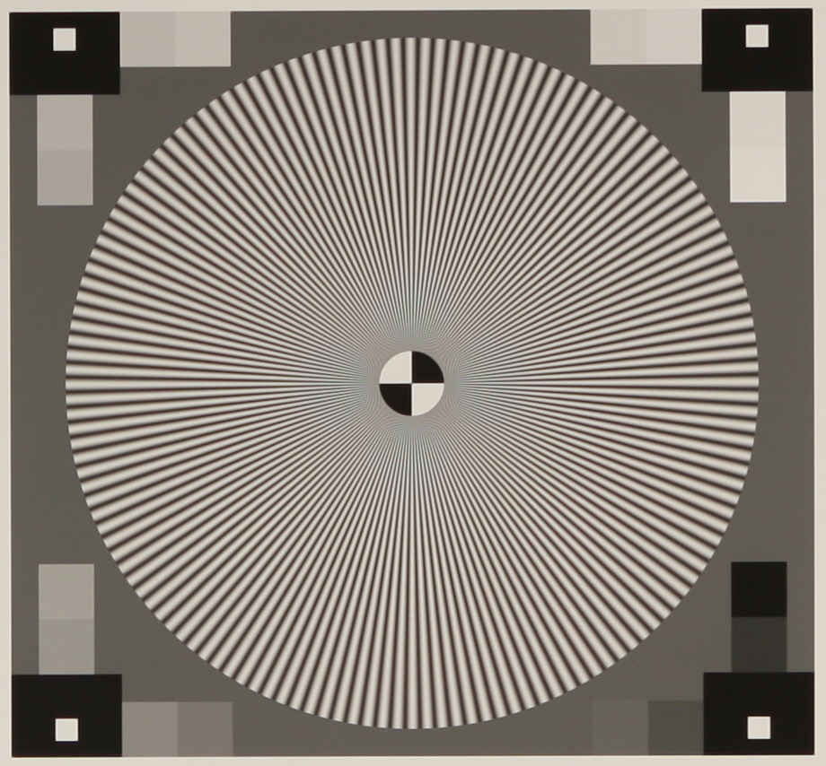
Star (black squares in corners) is the traditional design with density patches around the star and white squares inside larger black squares at the corners. Star (registration marks on extended sides), shown on the right, is a newer design that includes registration marks and slanted-edges on the sides. It works with Automatic ROI detection (selected in the ROI Options window). Star-only omits all extra graphics. Just the star and nothing more. |
 |
In Rescharts, select the pattern to analyze (in this case, Star Chart ) by clicking on the appropriate entry in the popup menu below or by clicking on if Star Chart is displayed. The button and popup menu (shown on the right) are highlighted (yellow background) when Rescharts starts.
Select the image to read. If the pixel size is the same as the previous Star Chart run, you’ll be asked if you want to use the previous ROI, adjust the previous ROI, or crop anew. If the folder contains meaningless camera-generated file names such as IMG_3734.jpg, IMG_3735.jpg, etc., you can change them to meaningful names that include focal length, aperture, etc., with the Rename Files utility, which takes advantage of EXIF data stored in each file.
Cropping The initial crop should include the entire pattern, including the outside of the black rectangles (with the small white squares inside). It doesn’t have to be precise because it will be refined in the ROI fine adjustment window, shown below. The ROI fine adjustment window may be maximized to facilitate fine selection.
In the ROI fine adjustment window the pattern should be cropped so
- the middle cyan square is at the bounds of the large star pattern circle (or slightly inside if there is distortion),
- the inner cyan square is on the inner circle (which consists of four quadrants— two white, two black) for inner circles with 1/10 the diameter of the outer. (The inner circle will be well inside of the inner cyan square for small inner circles, which have 1/20 the diameter.),
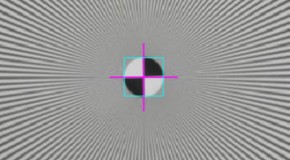
- the magenta crosshair inside the inner circle is well-centered. If it is slightly off Imatest will automatically correct it.
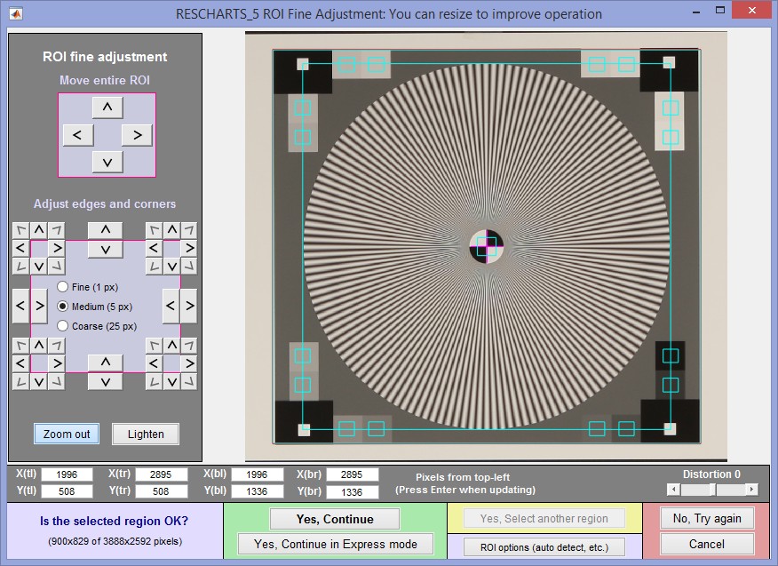 ROI fine adjustment window showing the cropped Star Chart image
Canon EOS-40D camera, 24-70mm f/2.8L lens set at 50mm, f/5.6, ISO 100.
Click here or on the image to load full-size test image.
|
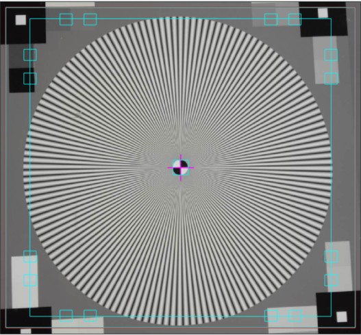
Distorted images The image on the right has significant keystone distortion. For such cases (including optical distortion – barrel or pincushion), make sure all the outer borders are inside the star and, most importantly, make sure the selected region is centered close to the center marker (indicated by the cyan square and magenta cross patterns), as shown below. |
 |
If Express mode is not selected, the input dialog box shown below appears. In Rescharts this dialog box can be at opened any time by pressing the button.
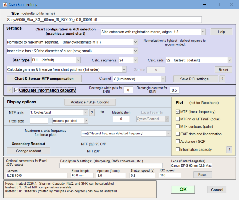 Star chart settings window
Settings
There is no setting for the number of chart cycles because it is automatically detected.
Chart configuration applies to the next run. You can choose between the traditional design, which has no registration marks, or newer designs that work with automatic ROI detection. It can also be selected from the Chart configuration dropdown menu in Rescharts.
Normalization selects the MTF normalization method (where to set MTF to 1.0):
- normalize to the outer MTF value for each segment (the default),
- normalize to the maximum outer MTF value in all segments, or
- normalize to the difference between the lightest and darkest of the grayscale square patches near the pattern edge. This often gives the best estimate. Does not work with bar (square wave) charts.
- Normalize by extrapolating smoothed MTF to 1 at f = 0 (OK for simple curves)
(1) may be slightly better when illumination is nonuniform. (2) may be slightly better when actual MTF varies between segments. (3) is usually better because the lowest spatial frequencies in the star may not be low enough approximate zero spatial frequency.
| Bar (square wave-modulated) patterns are analyzed similarly to sine patterns (which are usually recommended), but the correct normalization is required because the fundamental sine component (n=1) of a bar pattern (square wave) is 4/π times the bar pattern amplitude. |
The Fourier transform of a square wave of amplitude ±1 is \(\displaystyle x(t)=\sum^\infty_{n=1,3,5,\ldots} \frac{4}{n\pi} \sin(n\omega_0t)\) |
Normalization settings 1, 2, or 4 (but not 3 – Normalize to darkest-lightest outer square) work with bar star charts.
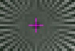 Inner circle May have 1/10, 1/20 the diameter of the outer circle or may be omitted (No inner circle). Should match the chart. Affects the maximum spatial frequency of the analysis. The inner circle consists of a registration mark (quadrant pattern), which is used to refine the region alignment. If it is omitted, you must be extremely careful to center the pattern (using a + indicator) when making the ROI fine adjustment.
Star type FULL (default) or Half-auto.
FULL assumes a full star with segment 1 centered at 0º.
Half-auto assumes a half or full star, automatically detected, but centers segments differently to correspond to the star orientation, so the first and last edges are located at multiples of 45º. Half-stars are a feature of the TE42 test chart, which will be supported by the Imatest Arbitrary charts module.
Calc segments is the number of segments around the circle to display in the analysis. Select 8 (the default; recommended for most work), 16, or 24. (16, which works better with half-stars, replaced 12 in Imatest 5.0.) Calc. segments should never be more than half the number of chart cycles. 8 is the best choice most of the time.
Calc. radii is the number of radii on the circle used for the MTF calculations. 64 is slightly more accurate than 32, but somewhat slower (it’s the default for now). 128 is slower, contains more frequencies than needed, and is more susceptible to noise. It is no longer recommended (and may be deprecated).
Enter or calculate gamma Choose between Calculate gamma & linearize from chart patches or Enter gamma for linearization. If Calculate gamma… is selected, the 16 small square patches at the periphery of the star chart are used to determine the value of gamma for linearizing the chart, Gamma (below) is disabled, and the displayed value of gamma includes the indicator (chart).
Gamma is used to linearize the test chart when Enter gamma… (above) is selected. It can be measured by Stepchart, Colorcheck, or Multicharts. 0.5 is a typical value for color spaces intended for display at gamma = 2 2 (sRGB, Adobe RGB, etc.). If gamma is entered (rather than calculated), the displayed value of gamma includes the indicator (input).
Channel is R, G, B, or Y (luminance; the default).
Calculate information capacity turns on the Shannon information capacity calculation (Imatest 2020.1+).
Display options
MTF units, etc. selects the x-axis units. If Cycles/inch or Cycles/mm are selected, the pixel spacing (um/pixel, pixels/inch, or pixels/mm) should be entered.
Maximum x-axis frequency for linear plots selects the maximum spatial frequency to be displayed in linear plots. Star chart is the only module other than the slanted-edge modules that can analyze MTF above the Nyquist frequency (0.5 cycles/pixel).
Secondary readout allows up to two secondary readouts (MTFnn, MTFnnP, or MTF at a specified spatial frequency) to be displayed on the MTF plots. Details here.
If you’re running from Rescharts, don’t worry about getting all settings correct: You can always open this dialog box by clicking on .
After you press , calculations are performed and the most recently-selected display appears.
Output
The Display box in the Rescharts window, shown below, allows you to select any of several displays. Display options are set in boxes that appear below Display. All displays except Exif data have a channel selection option (Red, Green, Blue, or Luminance (Y) (0.3R + 0.59G + 0.11B).
| Display | Description |
| MTF (original and linearized) | MTF for up to 8 segments of the star. Both linear and logarithmic frequency displays are available. |
| MTFnn or MTFnnP | Display MTFnn (the frequencies where MTF equals nn % of the low frequency values) and MTFnnP (the frequencies where MTF equals nn % of the peak value) for nn = 70, 50, 30, 20, and 10. Both polar (spider) and rectangular plots are available. |
| MTF contours (rectangular) | Display MTF contours in a rectangular plot with linear or logarithmic frequency display. Similar to the MTFnn rectangular plot. |
| MTF contours (polar) | Display MTF contours in a polar plot whose geometry duplicates that of the target. |
| EXIF data | Show EXIF data if available as well as linearization curves (used to calculate gamma from the chart). |
| In addition to the displays, two buttons allow you to save results. | |
| Saves an image of the Starchart window as a PNG file. If you check Display screen in the Save screen dialog box, the image will be opened in the editor/viewer of your choice. (Irfanview works well, and it’s free.) | |
| Saves detailed results in a CSV file that can be opened by Excel and also in an XML file. | |
The spatial frequency is automatically calculated from the image, under the assumption that log frequency increases linearly with distance. The number of chart cycles is also determined automatically.
MTF
The MTF (Spatial Frequency Response) can be displayed on a linear or logarithmic frequency scale. You can select between showing the first 8 segments equally weighted, or emphasizing any of the segments (Segment 1 is shown as a thick black line below). The average response is a thick magenta-gray line. Smoothed, interpolated response is normally displayed, but uninterpolated, unsmoothed (raw) response is available as an option.
Normalization: MTF is normalized (set to 1.0) using either (1) MTF at the outer radius of each segment, (2) the maximum value of MTF at the outer radii of all segments, or (3) the difference between the lightest and darkest square near the pattern edge. Neigher case (1) nor (2) is ideal because the minimum spatial frequency is not as low as it should be for correct normalization. (The high to low spatial frequency ratio is only 10 or 20 for the star chart — much lower than for the Log Frequency or Log F-Contrast charts.) In general, normalizing MTF to the outer radius of the star increases MTF slightly above its true value. MTF should ideally be normalized to a lower spatial frequency. Case (3) should only be used with maximum contrast patterns.
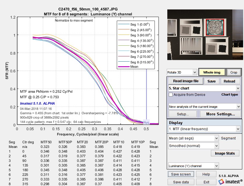 MTF (linear frequency scale) for 8 segments of the Star pattern
The entire Rescharts window is shown. The original 64 radii are linearly interpolated to 101 frequencies, then smoothed to eliminate response roughness caused by calculation artifacts and noise. Gamma = 0.454 (chart) at the lower left of the plot indicates that gamma was calculated from the 16 small square patches at the periphery of the chart. If it were calculated elsewhere and entered into Star Charts, (input) would be displayed instead of (chart).
MTF50, MTF50P, MTF20, MTF20P, MTF10, and MTF10P for the first 8 segments are displayed in a table below the plot for this and several of the output plots (but not shown below).
MTFnn, MTFnnP
The plot on the right shows MTF70 through MTF10 (spatial frequencies where MTF = 70,, 50, 30, 20, and 10%) on a linear frequency scale displayed in rectangular (Cartesian) coordinates. Frequency is displayed in cycles/pixel, but Line Widths per Picture Height (LW/PH), cycles/inch, or cycles/mm can be selected by pressing the button. The full circle is shown: segment 9 corresponds to segment 1: (0 degrees center angle). The legend (the box on the right) has been moved using the mouse to uncover the MTF10 (blue) line. |
 MTF70 – MTF10: Rectangular (Cartesian) coordinates, Linear frequency scale. |
|
|
The plot on the right shows MTF70 through MTF10 displayed in polar coordinates. Spatial frequency (cycles per pixel in this case) increases with radius. (This is the opposite of the image itself, where spatial frequency is inversely proportional to radius.) This plot is most similar to the spider plot shown in Image Engineering digital camera tests and Digital Camera Resolution Measurement Using Sinusoidal Siemens Stars (Fig. 15), by C. Loebich, D. Wueller, B. Klingen, and A. Jaeger, IS&T, SPIE Electronic Imaging Conference 2007. MTF10 (the black octagon on the right) corresponds to the Rayleigh diffraction limit. |
 MTF70 – MTF10: Polar coordinates, Linear frequency on radius. |
MTF contours: rectangular and polar
The plot on the right shows the MTF contours for each of the 8 segments. Spatial frequency is displayed on a linear scale, but a log scale may be selected and a color bar (see below) may be added. This plot contains information similar to the rectangular MTFnn plot, above. |
 MTF contours, rectangular display, Linear frequency scale. |
|
The plot on the right shows the MTF contours for each of the 8 segments, displayed on a polar scale, where location (radius) on the plot corresponds to the image. This is the inverse of the polar MTFnn plot, above, where spatial frequency is the inverse of image radius. Most of the action in this image is near the center. If the Zoom box is checked you can zoom in by selecting a portion of the image or simply by clicking on it. |
 MTF contours, polar display. |
EXIF data, linearization, & centering
The plot on the right shows
|
 EXIF summary, linearization, centering. EXIF summary, linearization, centering. |
Information capacity (Imatest 2020.1+)Calculate information capacity must be checked in the Settings window. Shannon Information Capacity contains further instructions and a detailed explanation of the calculation. Plots show
Information capacity (2.92 bits/pixel for this case) is shown below the plot. |
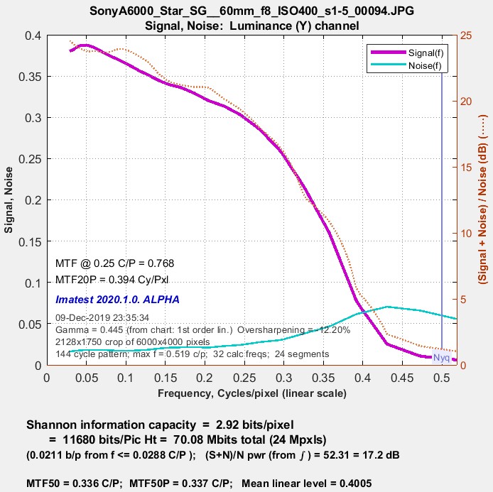 Shannon information capacity @ ISO 400 Shannon information capacity @ ISO 400 |
Difference image (noise-only, etc.) (Imatest 2020.1+)When Calculate information capacity is checked some remarkable results are available. Foremost among them is an image of noise inside the star, measured in the presence of the sinusoidal star signal. This image shows the noise of a JPEG image from 24-megapixel Micro Four-Thirds camera set to ISO 25600 (a very high ISO speed). Appearance is very different from a raw-converted TIFF from the same exposure, which has no noise reduction or bilateral filtering. Note: the orange circle represents the Nyquist frequency, fnyq. The strong cyan circles represent 0.5 and 0.25 fnyq. Several similar displays are available. |
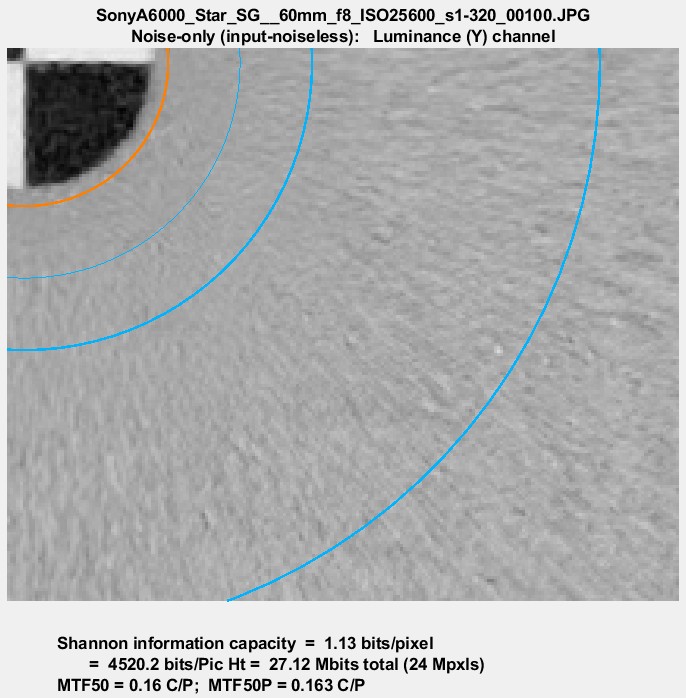 Noise near the center of a Siemens star image @ ISO 25600: measured with the signal removed. Noise near the center of a Siemens star image @ ISO 25600: measured with the signal removed. |
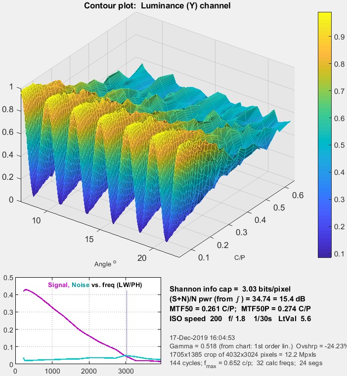
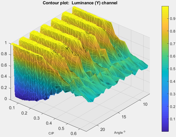
3D Surface plot (Imatest 2020.1+)To obtain this display, 3D Surface plot calculation (as well as Calculate information capacity) must be set in the settings window. It shows the signal (for the selected channel) as a function of angle and spatial frequency (in Cycles/Pixel), which is inversely proportional to radius. This plot represents a narrow pie-slice of the original image, with angular detail at high spatial frequencies greatly enlarged. A small plot of MTF and noise as a function of spatial frequency is displayed as well as a summary of key results (information capacity, etc.). This plot was motivated by tests on an iPhone 10, where the image appeared to be saturating at low to middle spatial frequencies, but the degree of saturation was difficult to assess by viewing the image. As we can see on the right, saturation is very strong, apparently as a result of some kind of local tone mapping. It is not evident in MTF curves from the star pattern or from the adjacent slanted edges. The iPhone had some Adobe software installed that allowed both raw (DNG) and JPEG software to be captured. We don’t know if this affected the JPEG processing. The image below shows the response of a TIFF file (converted from a DNG raw image from the same iPhone 10). The response is sinusoidal— well-behaved with no amplitude visible distortion. The information capacity is nearly identical to the distorted JPEG image, where several things are happening: random noise is zero where the image is saturated, but noise as defined by \(N(\phi) = S(\phi)-S_{ideal}(\phi)\) in Shannon Information Capacity, is increased by the amplitude distortion (deviation from the sine function). The insensitivity of information capacity to image processing, observed in other cases, is a remarkable result. By comparison, MTF50 and MTF50P is very much higher in the highly-processed JPEG image.
|
|

Sine vs. bar patterns.
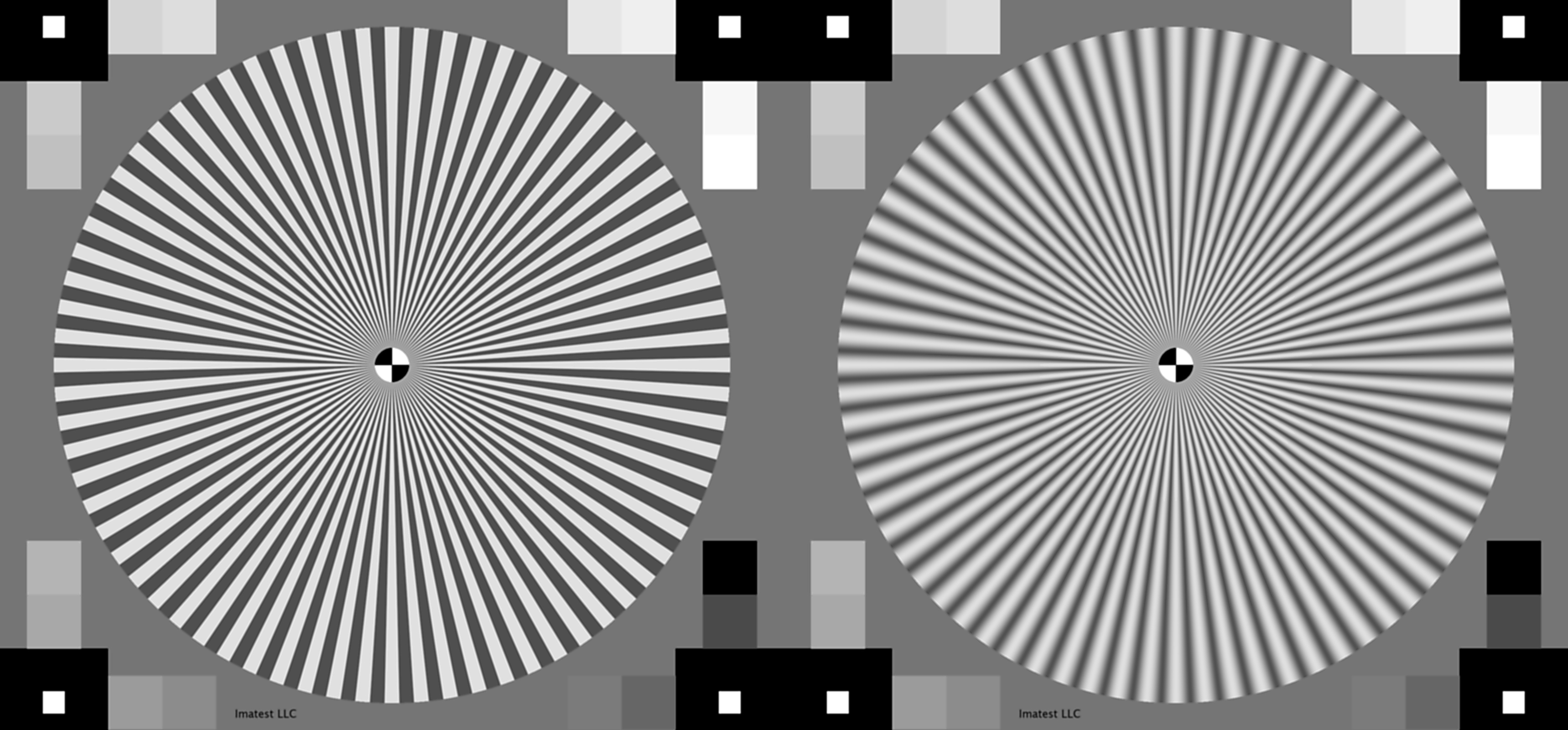
Bar and sine star patterns. Click on image to download.
Although we generally recommend sinusoidal Siemens stars, bar stars work equally well and give identical results as long as processing stays linear. The reason for this is that the algorithm (below) uses Fourier components, and hence only use fundamental frequencies. Harmonics, which are present in bar patterns but not sinusoidal patterns, are ignored. The image on the right was used to compare the two patterns. The individual patterns were produced with the Test Charts module set to pixel height = 1600 and contrast ratio = 10:1. The image was processed with Image Processing with Gaussian filter 2 set to 1.8 sigma and Sharpen (USM) set to Radius = 2, Amount = 1.4, and Threshold = 0.1.
You can click on the image, download it, then run Star (fixed or Rescharts) for the left (bar) and right (sine) patterns. We leave this as an educational exercise to the reader.
Equations, algorithm, and issues
|
Equations for analyzing the Siemens star are given in Digital Camera Resolution Measurement Using Sinusoidal Siemens Stars by C. Loebich, D. Wueller, B. Klingen, and A. Jaeger, IS&T, SPIE Electronic Imaging Conference 2007. The algorithms used for Imatest Star Charts are similar, differing only in details. The 32 or 64 radii ri , located from just outside the inner circle to just inside the outer circle, are selected using a logarithmic scale that makes them more closely spaced near the inner circle. This makes the frequency spacing (proportional to 1/radius) more consistent than for uniformly spaced radii. For each radius ri, all points P(φ,ri) are located with radii between \((r_{i-1}+r_i)) / 2\) and \((r_{i+1}+r_i)/2\) pixels. For a chart with Np cycles, spatial frequency is \(f = N_p / (2 \pi) \text{ cycles/radian} = N_p / (2 \pi \: r_i) \text{ cycles/pixel}\). Note that in the nomenclature of ISO 12233:2017, Appendix F, \(g = 2 \pi r_i / N_p = \text{ cycle length in pixels}\). This definition is inconsistent with equations (F.3) and (F.5): they only make sense if g is redefined to have units of cycle length in radians (not pixels), i.e., \(g = 2 \pi / N_p = \) = cycle length in radians. With this correction, \(2 \pi / g = N_p\) can be substituted into the equations below to give them the same form as (F.3) and (F.5). Points P(φ,ri) fit a curve for (pixel level) I as a function of angle φ in radians and radius ri in pixels, \(I(\phi,r_i) = a + b_1 \sin(N_p \phi) + b_2 \cos(N_p \phi) = a + b \sin(N_p \phi) + \theta), \text{ where }\: b = \sqrt{b_1^2 + b_2^2} \:\text{ and }\: N_p = 2 \pi / g\) \(\text{Modulation} = b / a\) The equation for I(φ,ri) is recognized as a term in a Fourier series expansion, which can be solved using the standard Fourier series equation since each segment (there are 8, 12, or 16) has an integral number of cycles (of a total of N = 144, 72, 48, 36, 24, or 16 cycles on the chart). \(b_1 = k \text{ mean}(P(\phi, r_i) \sin\bigl(N_p \phi \bigr));\) \(b_2 = k \text{ mean}(P(\phi, r_i) \cos\bigl(N_p \phi \bigr);\) \( a = \text{mean} ( I(\phi))\) The mean is taken over each segment. Since MTF is equal to Modulation normalized to 1 at the lowest measured spatial frequency for each segment (or all segments— see Normalization, below), k drops out of the final result. Algorithm issues Bumps in the MTF response curve caused by aliasing are visible in the image below. 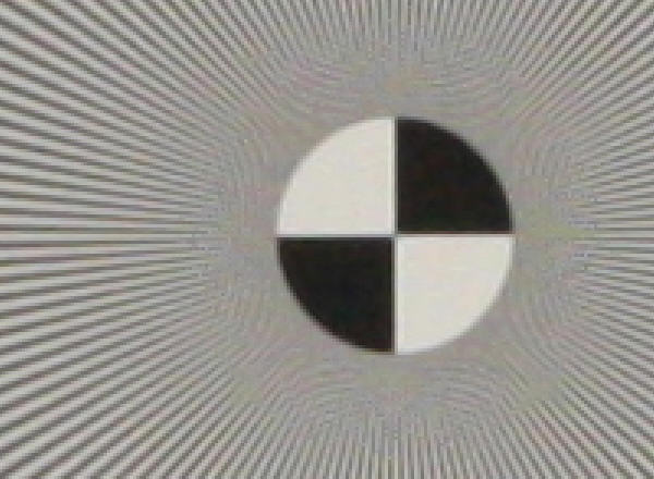 3x enlarged image of the center of a star pattern acquired on the Canon EOS-40D, 24-70mm f/2.8 lens set to 50mm, f/8 (a sharp setting) Normalization: MTF is normalized using (1) MTF at the outer radius of each segment, (2) the maximum value of MTF at the outer radii of all segments, or (3) the difference between the lightest and darkest square near the pattern edge. Neither case (1) nor (2) is ideal because the minimum spatial frequency is not as low as it should be for correct normalization. (The high to low spatial frequency ratio is only 10 or 20 for the star charts — much lower than for the Log Frequency or Log F-Contrast charts.) In general, normalizing MTF to the outer radius of the star increases MTF above its true value. MTF should ideally be normalized to a lower spatial frequency, as with case (3), which should only be used with maximum contrast charts. |
