Lens aberrations, diffraction, and defocus (or focus error) are basic factors that limit lens sharpness. They are described in the following sections.
Lens aberrations – Diffraction – Pixel response limits and Q – Visualizing Q – Defocus
Lens (Optical) Aberrations
Imperfections in optical systems arise from a number of causes that include different bending of light at different wavelengths, the inability of spherical surfaces (or even ashperes) to provide clear images over large fields of view, changes in focus for light rays that don’t pass through the center of the lens, and many more (i.e., coma, stigmatism, spherical aberration, and chromatic aberration (longitudinal and lateral)). Aberration correction is the primary purpose of sophisticated lens design and manufacturing, and it’s what distinguishes excellent from mediocre optical designs.
Optical aberrations (sometimes called Seidel Aberrations after a low-order mathematical model) can be broken down into five or six individual components. Imatest cannot separate them— that requires an (expensive) optical lens tester.
Lens aberrations tend to increase (become more difficult to correct) at large apertures (small f-numbers) and vary greatly for different lenses, even among different samples of the same lens; i.e., the quality control of mass-produced lenses does not always produce lenses of identical quality
Diffraction
Diffraction is a fundamental physical property that blurs images. It is caused by the bending of light waves near boundaries. The smaller the aperture (the larger the f-number), the worse the diffraction blur. Since diffraction is a fundamental physical effect, it is the same for all lenses. For most lenses, performance does not vary significantly at small apertures (large f-numbers), where diffraction is worse than aberrations. The f-number is equal to the lens focal length divided by its aperture diameter. In the classic f-stop sequence
{ 1 1.4 2 2.8 4 5.6 8 11 16 22 32 45 64 …}
each stop admits half the light of the previous stop, while the f-stop number is multiplied by the square root of 2 (1.414). When a photographer says, “I increased the exposure by one f-stop,” then the sequence is decreased by one step; e.g., the aperture changes from f/8 to f/5.6.
|
Aberrations tend to be worse at large apertures (small f-numbers), while diffraction gets worse at small apertures (large f-numbers). As a result, lenses tend to have an optimum aperture where they are sharpest, typically around 2 to 3 f-stops below a lens’ maximum aperture (often less for premium lenses). The optimum is fairly broad. |
You can find the optimum aperture by running a batch of images (Imatest SFRplus or eSFR ISO recommended) taken at different apertures, then entering the combined output (a CSV file) into Batchview (Figure 1).
Figure 1. Set of images taken at f/4.5 to f/22
In Figure 1, bars show MTF50 in line widths per picture height (LW/PH) for the weighted mean (black), center area (red), part-way area (green), and corners (blue). The procedure is described in detail here. For the lens results in Figure 1, the optimum aperture (f/8 to f/11) is 2 to 3 stops from the maximum and edge sharpness is unimpressive.
In Figure 2, diffraction-limited MTF is displayed as a pale brown dotted curve in the MTF figures produced by SFR, SFRplus, and eSFR ISO when the pixel spacing (usually in microns) has been manually entered in the appropriate dialog box and the aperture (f-number) is known (it’s normally retrieved from the EXIF data, but can be entered manually).
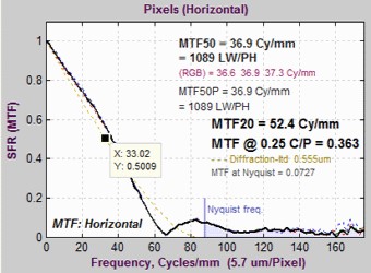
Figure 2. MTF plots showing diffraction-limited MTF (as a pale brown dotted line)
In this figure, the curve on the left is for the Canon EOS-40D (5.7-micron pixel spacing) with the lens set at f/22, which is a small aperture that should only be used when large depth of field is required and sharpness can be sacrificed.
Diffraction causes a point of light to spread out, forming a circular pattern called an Airy disk. The full equation (Wikipedia) is shown below. The radius of the disk (center to first null) is quite simple.
\(\displaystyle r_{airy} = 1.22 \ \lambda N\) where λ is the wavelength and N is the F-number (f-stop = aperture diameter/focal length) of the lens.
The equation for diffraction-limited MTF can be found below and in Diffraction Modulation Transfer Function from the SPIE OPTIPEDIA, David Jacobson’s Lens Tutorial (older version), and normankoren.com. The diffraction cutoff frequency is
\(\displaystyle f_{\mathit{cutoff}} = \frac{1}{\lambda N}\)
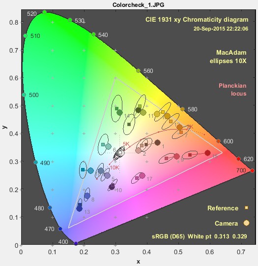
CIE 1931 chromaticity diagram showing colors & wavelengths
λ is typically 0.555 microns (0.000555 mm) for visible light (yellow-green; the approximate wavelength where the eye is most sensitive), but it can be changed for cameras with different spectral response (such as Infrared).
Let
\(\displaystyle s=\frac{f}{f_{\mathit{
The diffraction-limited MTF is
\(\displaystyle \mathit{MTF}_{\mathit{
\(\displaystyle \mathit{MTF}_{\mathit{
Figure 2 is also shown with a Data Cursor Datatip, which allows you to examine plot or image pixel values. The Data Cursor Datatip is available in all figures and interactive GUIs in Imatest 3.6+.
Lens MTF response can never exceed the diffraction-limited response, but system MTF response often exceeds it at medium spatial frequencies as a result of sharpening, which is (and should be) present in most digital imaging systems.
In addition to lens response, system MTF response is affected by the sensor (which has a null at 1 cycle/pixel), the anti-aliasing filter (designed to suppress energy above 0.5 cycles/pixel), and signal processing (which can be very complex and can be different in different regions of an image).
Diffraction, pixel size, and test chart requirements
Imatest MTF tests are performed by photographing and analyzing test charts— most often slanted-edge charts. We have made a strong effort to ensure that chart quality is sufficient to give accurate results. We recently (August 2021) realized that because of the diffraction limit, chart size requirements can be relaxed somewhat for cameras with tiny pixels, roughly defined as under 1.2 microns.
In developing the procedure for dealing with diffraction, we note that the spatial frequencies where diffraction-limited MTF equals specified values (fnn for MTF = nn%) are a simple fractions of \(f_{\mathit{cutoff}} =1/(\lambda N)\)
\( f_{90} = 0.0786 /(\lambda N); \ \ \ \ \ f_{70} = 0.237/(\lambda N); \ \ \ \ \ f_{50} = 0.404/(\lambda N); \ \ \ \ \ f_{30} = 0.585 /(\lambda N)\)
For pixel size p, \(f_{Nyq} = 1/(2p)\)
If \(f_{30} < f_{Nyq}\), the best possible sharpness of the lens is less than we normally assume. This allows Sensor height in pixels (the left y-axis in the figures in Test chart suitability for MTF measurements) to be multiplied by \(f_{30} / f_{Nyq}\), which reduces the recommended chart height.
The full procedure explained and illustrated for a 108MP sensor with really tiny 0.7 μm pixels and an f/2 aperture, in Test chart suitability for MTF measurements.
Diffraction, pixel response limits, and Q
The question naturally arises, “When is a camera’s resolution limited by the optics, and when it it limited by the sensor pixel size?” In other words,
What is the boundary between diffraction-limited and sensor pixel size-limited optical systems?
The question can be addressed with the concept of Q, presented in “Modeling the Imaging Chain of Digital Cameras” by Robert Feite, SPIE Digital Library, 8.3., (Special thanks to J. Gordon Arkenberg for pointing this out to me.)
Essentially, Q is the ratio of the sensor cutoff frequency frequency \(f_\mathit{sensor-cutoff} = 1/p\), which is twice the Nyquist frequency fNyq, to the diffraction-limited cutoff frequency \(f_{\mathit{cutoff}} =1/(\lambda N)\).
\(\displaystyle Q = \frac{f_\mathit{sensor-cutoff}}{2 f_{Nyq}} = \frac{\lambda (f/\#)}{p} = \frac{\lambda N}{p} = 2 \lambda N f_{Nyq} \)
When Q = 2, \(f_{\mathit{cutoff}} =1/(\lambda N) = 1/(2p) = f_{Nyq}\), which is the highest frequency where image energy can be reproduced correctly, without aliasing.
To quote Feite, “Cameras with Q < 2 have a higher MTF but introduce aliasing, whereas cameras with Q > 2 have a lower MTF and produce blurrier images, but have no aliasing.” So for Feite, Q = 2 is the dividing line. In Imatest’s (mostly NLK’s) experience, a small amount of aliasing improves sharpness, but does not introduce unacceptable visual artifacts, so a lower Q is acceptable. I consider a system with MTF @ fNyq = 0.3 (30%) to have acceptable visual artifacts but potentially excellent perceptual sharpness. At this level,
\(\displaystyle f_{30} = 0.585/(\lambda N) = f_{Nyq} = 1/(2 p)\) ; hence
\(\lambda N / p = Q = 2 \times 0.585 = 1.17\)
This is significantly lower than Q = 2 , which ensures zero aliasing at the expense of perceptual sharpness. Q should not be thought of as a quality factor.
When the imaging system has no aliasing, i.e., the diffraction limit ≤ the Nyquist frequency (Q = 2),
the radius of the Airy disk will be nearly five times larger than the pixel spacing.
The image will not appear to be sharp at the pixel level.
Note that the Airy disk diameter is \(d_{airy} = 2 \ r_{airy} = 2.44 \ \lambda N = 2.44\ Q p\). At Q = 2 (no aliasing), dairy is 4.88 pixels wide. At Q = 1 (where the diffraction and sensor cutoff frequencies are identical), dairy is still 2.44 pixels.
Q is closely related to Depth of Field (DoF), which will not be discussed in detail on this page because it involves lens focal length and camera Field of View (which is used in defining the FoV limits). Briefly, large DoF requires small apertures with high values of Q, which may limit the sharpness.
While Q is not of direct concern to Imatest testing, it affects lens and system design and the interpretation of Imatest results. Examples:
- Cameras used in flatbed scanners, bar code readers, and certain medical devices (e.g., endoscopes) may use fixed-focus lenses and require large depth of field. They often have built-in light sources. The small apertures (large f/numbers) allow relatively little light to enter the lens, but the built-in light sources provide adequate illumination. These systems tend to have high values of Q. Their expected sharpness (when they’re in focus) can be considerably lower than the pictorial cameras described below.
- Cinema cameras often require very narrow DoF (to keep backgrounds uncluttered). This means large aperture lenses (set to large apertures) that typically have small values of Q.
- Most pictorial cameras (consumer cameras) have lenses than can be focused (either auto or manual focus), and are expected to produce sharp images. These include small cameras with large aperture prime lenses (typically around f/2) as well as larger cameras (DSLR and mirrorless) with adjustable apertures. These cameras have values of Q well under 2; often under 1.
We have been looking at a 108 megapixel camera with 0.7 micron pixel size and an f/2 aperture, which admits a large amount of light. F/2 apertures are relatively common in small (mobile) cameras, and are often diffraction-limited. Increasing the aperture (decreasing the f/number), makes it difficult to achieve diffraction-limited performance because lens aberrations start to dominate. This camera has Q = 0.555 × 2 / 0.7 = 1.59.
Lenses in cameras with large pixels and sensors— mirrorless and DSLR cameras with 1 inch or larger sensors— are rarely diffraction-limited at their maximum aperture. The have low values of Q, normally well under 1 at their maximum aperture, but due to aberrations at large apertures they have have an “optimum aperture”, usually about 2 stops (twice the f/number) below the maximum, after which they tend to slowly approach diffraction-limited performance.
Visualizing the effects of Q
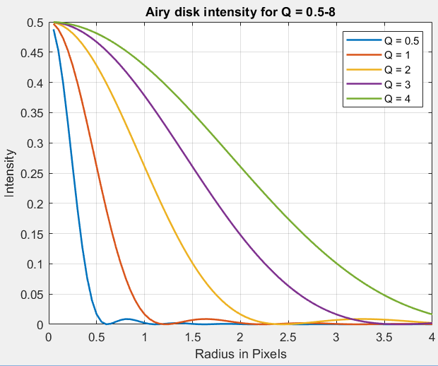
The effects of Q can be visualized by normalizing spatial units to pixels and frequency units to cycles/pixel (C/P). The general equation for the Airy disk from Wikipedia is
\(\displaystyle I_{Airy} = \left[ \frac{2 J_1(x)}{x} \right]^2 \) where \(\displaystyle x = k a \sin{\theta}; \ \ \ \ k = 2 \pi/\lambda \)
J1 is a Bessel function of the first type, easily evaluated with the MATLAB besselj function. The Jacobson tutorial leaves off the square. We assume small angles, so that \(\displaystyle \sin(\theta) \cong \theta \cong r/f\), where A = 2a is the aperture diameter, f is focal length, ν is spatial frequency (ν avoids confusion with focal length f ), and r is radius (distance from the center of the disk). Using \(\displaystyle Q = \lambda N / p, \ \ \ x = \pi r / Q p \), Note that r/p is distance from the Airy disk center normalized to units of pixels.
The OTF of the Airy disk (where MTF = |OTF|) is
\(\displaystyle OTF(\lambda,N,\nu) = \frac{2}{\pi} \left[ \arccos(\lambda N \nu) – \lambda N \nu \sqrt{1-(\lambda N \nu)^2} \right], \ \ \ \ \ \ \lambda N \nu \le 1\)
= 0 otherwise
Again, noting that \(\displaystyle Q = \lambda N / p, \ \ \lambda N \nu = p Q \nu \), where pν is spatial frequency in cycles/pixel.
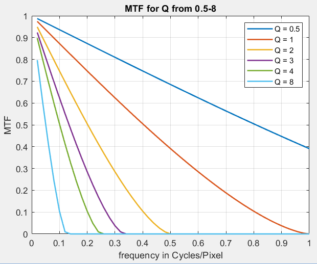
IAiry and MTF as functions of Q are plotted below.
|
|
|
Defocus
Defocus (or misfocus or focus error) blurs the image — taking a bite out of MTF. Defocus is a large subject that we can only touch on.
In a hypothetical perfect world (with no diffraction or lens aberrations), defocus causes a spot of light to be imaged as a simple disk, called a circle of confusion, described in Wikipedia. Depth of field (DoF) — the range of distances where the scene appears to be in focus — is defined by specifying a maximum circle of confusion, which is a function of geometry: lens focal length and f-number, subject distance, and, most importantly, where the lens is focused. The latter parameter — lens focus — is frequently subject to error.
In the old days, DoF was defined as the range of object distances where the circle of confusion in an 8×10 inch print was under 0.2 mm. This definition was useful in the age of film, where lenses were often not as good as they are today (with a few exceptions), big enlargements were difficult to make, and the film itself did not stay flat: its position could vary. Stopping down the lens (increasing the f-number) increases the depth of field, but often at the expense of sharpness where the lens is in good focus (thanks to diffraction). Some applications, like landscape photography, look best with large DoF, but others, like portraits and cinema, look better with small DoF (which can blur out cluttered, distracting backgrounds). As we said, this can be a big subject.
Fixed focus lenses — Most consumer cameras have autofocus (or focusable) lenses, but we have recently encountered cases where the focus is fixed, usually either at infinity or the hyperfocal distance — where the lens is focused so so the far DoF limit (however it happens to be defined) is at infinity. These lenses are primarily used in the automotive industry or for aerial photography. When we encounter them, we have to determine if we can effectively test them in the limited space of our facility.
The first step is to determine the circle of confusion diameter c for the camera at the specified test distance. Using Wikipedia’s notation, where f = focal length, A = Aperture diameter, N = f-number = f/A, and S1 = lens-to-object distance,
\(\displaystyle c = \frac{fA}{S_1 – f} = \frac{f^2}{N(S_1-f)} \)
Example: an aerial camera with a pixel pitch of 3.76μm (0.00376mm) has a 110mm f/4 lens focused at infinity. We would like to know if it can be reliably tested at 100 meters. Using units of mm,
c = 1102 / (4*(100000-110)) = 12100/(4*99890) = .0303mm = 30.3μm = 8.05 pixels.
This seems large, but we need to relate this to MTF degradation to determine how bad 100 meters is.
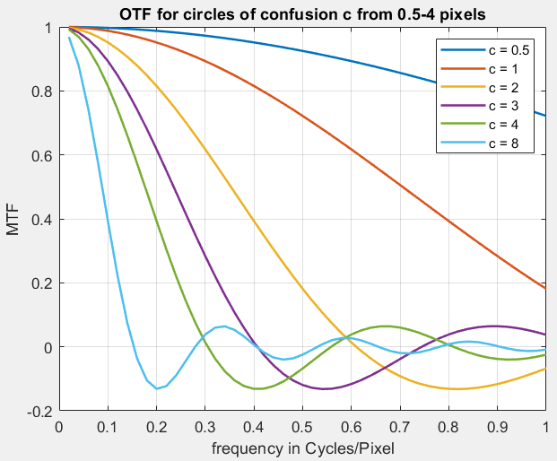
MTF in C/P for several circle of confusion diameters (c)
MTF for defocus
Going back to the Jacobson lens tutorial and noting that MTF = |OTF| (the modulus of the Optical Transfer Function, which includes phase): a negative value of OTF indicates a phase shift,
For a circle of confusion with diameter c, and spatial frequency ν (in compatible units to c, i.e., pixels and cycles/pixel)
\(\displaystyle OTF= 2J_1(\pi c \nu)/(\pi c \nu)\),
where J1 is a Bessel function of the first type, easily evaluated with the MATLAB besselj function. There is also a useful approximation:
J1 ≅ sin(0.84 πcν)/(0.84 πcν) up to the first null (0.84 πcν < π).
MTF vs spatial frequency in cycles/pixel for several values of c is shown on the right, which requires some interpretation. Typical high quality lenses have MTF50 around 0.3 cycles/pixel (this is very approximate), with MTF roughly 10-30% at the Nyquist frequency (fNyq = 0.5 C/P). MTF50 below 0.15 indicates an inferior (or misfocused) lens. MTF at Nyquist > 0.4 may be a little too sharp for the system: there can be significant aliasing effects and lens is probably more expensive than needed. With this knowledge we can say that
- c = 0.5 has no significant effect on measurements.
- c = 1 (MTF @ fNyq = 0.72) has a slight effect, but it is not significant in most cases.
- c = 2 (MTF @ fNyq = 0.19) has some effect on measurements, but is serious only for extremely sharp lenses.
- c > 2 should be avoided.
To find the distance S1 for a specified circle of confusion c, the above equation must be inverted.
\(\displaystyle S_1 = f + \frac{f^2}{Nc} \)
Example: for the above camera, if we want to find the distance for c = 2 pixels = 7.52μm = 0.00752mm,
S1 = 110 + 1102/(4*0.00752) = 402371mm ≅ 402.4 meters. This seems enormous (and it surprised us), but our tests confirm the math.
OTF for combined diffraction and misfocus — can be found on page 10 of the Jacobson lens tutorial. It’s a complicated equation (and not the product of the OTFs for diffraction and misfocus). For ν = spatial frequency = fsp, s = λNν, and a = πνc, where units are consistent (i.e., fsp = ν in cycles/mm for λ and c in mm).
\(\displaystyle OTF = \frac{4}{\pi a} \int_{y=0}^{y=\sqrt{1-s^2}} \sin\left(a \sqrt{1-y^2}-s\right)dy, \ \ \ \ s < 1\)
\(\displaystyle = 0; \ \ \ \ \ \text{otherwise}\)
A result for a small aperture is shown in the tutorial.