Postprocessor for viewing summaries of SFR, SFRplus,
Checkerboard, and eSFR ISO results
|
News — Imatest 25.1 (available in an alpha version before it is released) Batchview has been significantly upgraded and refreshed.
|
Introduction to Batchview
Batchview is a postprocessor for displaying lens test results generated by SFR, SFRplus, eSFR ISO, Checkerboard, and SFRreg batch runs (analyses of groups of test chart images taken at various apertures, focal lengths, Exposure Indices (ISO speeds), etc.). It can store and display up to four groups of results for convenient comparisons.
| Postprocessor comparison Each lets you compare sharpness of different regions and/or images |
|
| Postprocessor to SFR, SFRplus, and eSFR ISO. Input is two CSV results files for individual regions. Lets you compare individual edges from any region of any two images (or the same image). Displays MTF for both images and transfer function (A/B) or (B/A). | |
Image Stabilization/ Sharpness Compare |
Postprocessor to SFRplus-only. Input is two or three JSON results files. Image Stabilization must be checked in the SFRplus settings window. The region selection must be the same for all the files, but files may have different sizes. Lets you compare sharpness of regions (in approximately the same location) or of the image as a while. Can compare sharpness of two image files or calculate the effectiveness of (Optical) Image Stabilization using three image files. |
| Postprocessor to SFR, SFRplus, eSFR ISO, Checkerboard, and SFRreg (primarily the latter two) that lets you compare summary results for several files run as a batch and stored in a file whose name has the form root file_sfrbatch.csv or json. Most useful for measuring sharpness at the center, part-way, corners, and weighted mean for a range of apertures, but very versatile: it can analyze any image sequence. | |
| Postprocessor for eSFR ISO, Checkerboard, and SFRplus (auto-detect slanted-edge modules that calculate magnification) that lets you calculate measurement results from batches images acquired at different distances or with different focus settings. For measuring depth of field (DoF), curvature of field, and longitudinal (axial) chromatic aberration (which varies with distance, rather than radius, for the familiar lateral chromatic aberration). Lens Focal Length (FL) can be calculated precisely when the distance increment (from the motorized modular test stand) is known. Results for batches of several files are stored in a file whose name has the form root file_sfrbatch.json. |
|
Typical use: You’ve tested a lens at a range of apertures (for example, f/2.8, f/4, f/5.6, f/8, f/11, and f/16) at several focal lengths with SFR or SFRplus. To get a good feeling for its performance, you’ve measured its sharpness (MTF) at the center, corners, and part-way to the corners (ideally, selecting 9 regions in SFR; 13 or more in SFRplus). That’s a whole lot of data– at least 54 MTF curves for each focal length. You want to see a nice, concise summary.
The image below shows MTF50 in Line Widths per Picture Height (LW/PH)— a good measure of total image sharpness)— of four sets of tests (batches of runs).
- (A-B) The Canon 17-85mm lens on the EOS-40D at two different focal lengths.
- (C-D) The Canon 24-70mm f/2.8L and 24-105 f/4L on the EOS-5D Mk II, both at 70mm focal length. The 24-105 appears to have an autofocus defect.
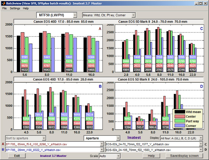
Batchview display from four sets of tests on different cameras and lenses
Note that the legend (Plot D; lower right) can be moved to uncover the numbers (LW/PH results).
The black, red, green, and blue bars are the weighted mean, the mean of the center region, the mean part-way out, and the mean of the corners, respectively. Numeric values displayed near the base of the bars are optional(they can be turned of in the Settings dropdown menu if desired).
If a single Display is chosen (selected in the Display box on the right, just below the plots), more detail is displayed.
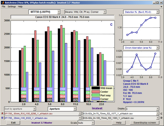
Batchview display from one set of tests
Two small plots (SMIA TV Distortion and Chromatic aberration area in %) and some EXIF data (metadata) from the first file in the batch are displayed on the right.
Preparing to run Batchview
The first step is to acquire one or more batches of test chart images— sequences of images in which one parameter is varied (most often aperture, i.e., f-stop, but focal length, ISO speed, etc., can also be varied), usually with most other parameters fixed. (Of course if aperture is varied, exposure time must also be varied to keep exposure constant.) You can use one of the composite charts illustrated in The Imatest Test Lab, but the most convenient and consistent results are obtained with the SFRplus chart, shown below inside the SFRplus setup window in Rescharts, which must be run to save settings prior to doing a batch run for several files in (the automatic, non-interactive version of) SFRplus.
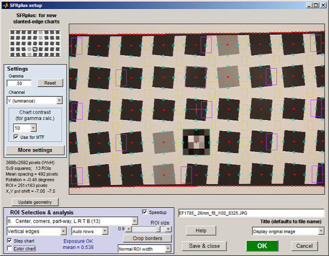
Rescharts SFRplus window showing settings used for the above Batchview run:
9 regions (1 center, 4 part-way, 4 corners)
SFRplus: The following settings are recommended when you run SFRplus in Rescharts. (Full instructions for running Rescharts can be found here).
- Select at least 9 regions (Center, corners, part-way) for optimum results. 13 or 23 are slightly better, but slower. Speedup can be checked.
- Chart contrast (typically 10 for SFRplus charts) should be entered. It may be used to calculate the camera gamma used to linearize the image for analysis (the results do not depend strongly on gamma).
- Vertical edges are recommended because they generate better chromatic aberration measurements– they’re close to tangential near the sides. Either can be used. Vertical and horizontal edges usually produce similar results for still cameras but sometimes differ for video cameras.
- Open to view additional settings. Most have no direct effect on Batchview. We recommend checking Close figures after save. The input file to Batchview(…sfrbatch.csv) is always saved for batch runs.
When the settings are correct, click to save the settings without running SFRplus or click to save settings and interactively run the selected file. Then press in the Imatest main window and select the batch of files to analyze. A maximum batch size of six is allowed in Imatest Studio.
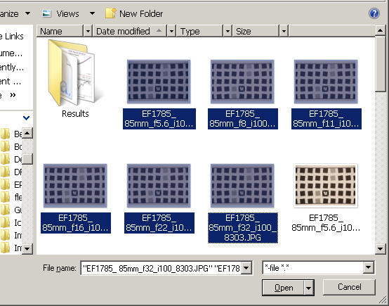
Read images dialog box, showing a batch of 6 files (form f/5.6 to f/32)
Use the View/Rename files module to change the meaningless names generated by the camera to more meaningful names that contain key EXIF data such as the aperture, focal length, etc. The file names in the above illustration were processed through View/Rename files.
SFR can also be used to generate input for Batchview, especially with targets that contain slanted-edges near the center, part-way out, and near the corners. The composite target shown below works quite nicely and also includes the Log F-Contrast and Star charts.
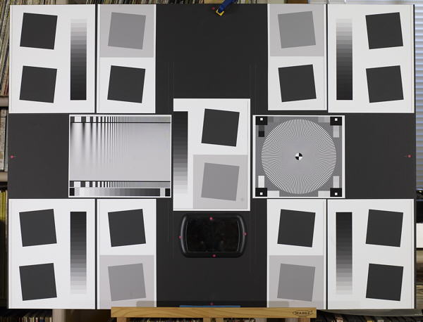
Sharpness target (30×40 inch) for cameras up to about 16 megapixels.
Details in The Imatest Test Lab.
Instructions for running SFR with this chart can be found in Using SFR Part 2. The sections on Repeated runs, Multiple ROI fine adjustment, and Automatic ROI refinement contain some helpful tips.
Running Batchview
To run Batchview, click the button in the Imatest main window. Initially, a blank screen will appear. In succeeding runs, saved file names will be read in, and a display will appear on the screen.
Empty Batchview opening screen
Enter the batch summary file(s), whose names have the form rootname_chan_sfrbatch.csv, into one of more of the file name windows (A, B, C, or D) at the bottom of the Batchview window. Rootname is typically the root name of the first file in the batch (the file name omitting the extension). Chan is the channel: Y (luminance), R, G, or B.
When files have been entered into the file name window(s) corresponding to the Display menu (lower right), the results will appear. Here is an example showing results for A and B in Imatest Studio.
Batchview results with two displays (Imatest Studio)
The plots are displayed side-by-side if you click Settings and uncheck 2 plots on top, bottom.
A large number of display options are available.
X-axis (independent variable; in the center below the plots)
Sets the independent (X) axis. All except numbers are derived from EXIF data. If EXIF data is not available, the numbers can be added by editing the sfrbatch.csv file in Excel of Open Office.
| Camera | Camera name |
| Lens | Lens description |
| Exposure Index (ISO Speed) | |
| Focal length | in mm |
| Shutter speed | in seconds |
| Aperture | (same as f-stop) The most commonly used independent variable; shown in the examples on this page. |
| Numbers (1,2,3, …) | Simple numeric sequence: 1, 2, 3, … |
| File name | |
| Short file name | Some of the text common to all the file names is not displayed. |
Sort order (Left, below the plots)
The X-axis order of plots usually needs to be specified (the default order determined by Windows rarely makes sense). The settings are Standard order, Reverse order (these two from Windows), Sort by aperture, Sort by shutter speed, Sort by Exposure Index, Sort by focal length, Sort by camera, and Sort by image file name. For most of the examples on this page, Sort by aperture has been selected.
Scaling (Bottom-center; Auto or manual)
Although Automatic scaling is the default, manual scaling can be specified so that all plots have the same y-axis scale. Scaling is selected in the small Scale dropdown menu at the bottom-center, which is set to Auto by default. If you select Enter, a small window appears to the right that allows you to enter the maximum y-value for manual scaling. For example, selecting 3000 sets the maximum y-value of all graphs. You can switch back to Auto whenever you want.
Display (lower right)
(both Studio and Master): A, B, A (top), B (bottom). (Master-only): C, D, C (top), D (bottom), All four : A (UL), B, C, D (LR). If a single file is chosen for display, two plots are displayed on the upper right and a summary of EXIF data for the first file is displayed to the right of the image (shown above).
Display variable (dependent variable; left of center above the plots)
This key setting determines what is displayed. The most common choice is MTF50 in Line Widths per Picture Height.
| MTF50 (LW/PH) | Spatial frequency for where MTF (contrast) is 50%, measured in Line Widths per Picture Height. The best indicator of overall perceptual sharpness of the total image. |
| MTF50 (Cy/Pxl) | MTF50 measured in Cycles per pixel. Indicates how well pixels are used. |
| MTF20 (LW/PH) | Spatial frequency for where MTF (contrast) is 20%, measured in LW/PH. Closer to the traditional vanishing resolution (~MTF10) than MTF50. (In digital systems MTF10 is often in the noise or above the Nyquist frequency). |
| MTF20 (cy/Pxl) | |
| MTF50P (LW/PH) | Spatial frequency where MTF is 50% of its peak value. The same as MTF50 except for strongly sharpened images, which have a peak in MTF response. Sharpening significantly increases MTF50. MTF50P is somewhat less affected, hence may be a better indicator of the true performance of strongly sharpened imaging systems. |
| MTF50P (Cy/Pxl) | |
| Peak MTF | Peak value of MTF. Usually 1, but can be larger for strongly sharpened systems. |
| R1090 (/PH) | 10-90% rise distance of the average edge in units of (10-90%) rises per picture height. Closely tracks MTF50. |
| R1090 (pxl) | 10-90% rise distance in pixels. Approximately inversely proportional to MTF50. |
| LSF PW50 (pxl) | 50% pulse width of the Line Spread Function (derivative of the edge) in pixels. |
| CA (pxl) | Lateral Chromatic Aberration (LCA) area in pixels. CA area is closely related to its visibility. But area in pixel units is not recommended because it is strongly affected by location. |
| CA (area %) | LCA area in units of percentage of the distance from the image center to the corner. Somewhat dependent on location, but much less so than when pixels are chosen as the units. May be strongly affected by raw conversion algorithm. |
| CA (crossing %) | LCA measured by the maximum distance between the transition centers of the three channels in center-to-corner %age. |
| CA (R-G %) | LCA measured by the distance between the transition centers of the Red–Green channels in center-to-corner %age. |
| CA (B-G %) | LCA measured by the distance between the transition centers of the Blue–Green channels in center-to-corner %age. |
Display regions
This selects the regions represented by the bars in the plot. The first, which selects a weighted mean of the regions (100% for the center region, 75% for the part-way region, 25% for the corner region) and each of the three regions is the most common selection.
| Means: Wtd Ctr, Pt wy, Corner | Display four bars: The black, red, green, and blue bars are the weighted mean, the mean of the center region (<30% ctr-corner), the mean part-way out (30-75% ctr-corner), and the mean of the corners (>75% ctr-corner), respectively. |
| Weighted mean | One bar displaying the weighted mean. |
| Center mean | One bar displaying the value in the center region (<30% of the center-to-corner distance). |
| Part way mean, worst | Two bars displaying the mean and worst-case value, part-way to the corner. (Worst case MTF is the lowest; worst case Chromatic Aberration is the highest). |
| Corner mean, worst | Two bars displaying the mean and worst-case values in the corner region. |
| Center, Pt wy, Corner means | Three bars displaying the means of the three regions |
| Part way mean | One bar displaying the value in the part way region (30-75% of the center-to-corner distance). |
| Corner mean | One bar displaying the value in the corner region (>75% of the center-to-corner distance). |
Region locations are shown below.
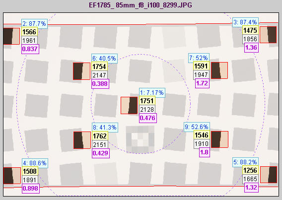
Multi region summary showing center region (inner circle)
and corner region (outside outer circle).
Plots on right (for single batch display)
When a single plot is selected, two small additional plots appear on the right. This enables you to present a rather complete set of results, for example (as shown above), sharpness on the main (large) plot, distortion in the upper-right plot, and chromatic aberration in the middle-right plot. The following parameters are available for the small right plots.
| Distortion % | SMIA TV distortion in %. Positive is pincushion; negative is barrel. |
| CA (area %) | LCA area in units of percentage of the distance from the image center to the corner. Somewhat dependent on location, but much less so than when pixels are chosen as the units. May be strongly affected by raw conversion algorithm. |
| CA (crossing %) | LCA measured by the maximum distance between the transition centers of the three channels in center-to-corner %age. |
| CA (R-G %) | LCA measured by the distance between the transition centers of the Red–Green channels in center-to-corner %age. |
| CA (B-G %) | LCA measured by the distance between the transition centers of the Blue–Green channels in center-to-corner %age. |
| Statistics (mean, sigma) | The mean and standard deviation (sigma) of the selected plot(s). Has been used to study consistency statistics. |
Settings dropdown menu
- Display bars (normally checked) Results are displayed as bar plots (shown in all examples on this page).
- Display lines (normally unchecked) Results are displayed as line plots.
- Small/Normal/Large/X-Large fonts Select font size. Larger fonts may be appropriate when the Batchview window is maximized for demonstrations.
- Edit titles Edit the plot titles, which default to Camera name, lens type, focal length. The titles may also be edited for display by typing directly in their boxes.
- Display numbers (normally checked) Turns on the display of numbers on the plot near the base of the bars.
- Reset screen Restore the screen to its original size and position.
- 2 Plots on Top, Bottom (normally checked) When checked and two plots (A,B or C,D) are selected, plots are stacked vertically, one on top of the other. When unchecked, plots are displayed side-by-side.
- Display LW/PH / Display LP/PH These settings switch between Line Widths/Picture Height and Line Pairs/Picture Height display.
- Distortion, CA in single plots (normally checked) If unchecked, the Distortion and Chromatic Aberration are displayed on the right of single plots. May be unchecked for displaying large groups of results where distortion and CA may not be of interest.