Image Processing for Image Information Metrics

Current Documentation
View previous documentation
View legacy documentation
All documentation versions

The basic premise of this work is that Information capacity is a superior metric
for predicting the performance of imaging systems.

It is better than sharpness or noise, which it incorporates, and it can be used
to derive metrics for measuring object and edge detection performance
and for designing electronic filters that optimize system performance.

Related pages

Image Information Metrics: Information Capacity and more contains key links to documentation, white papers, news, and more on image information metrics.

The paper from Electronic Imaging 2024, Image information metrics from slanted edges, contains the most complete exposition of the image information metrics. The material is also covered in various levels of detail in the three white papers linked from Image Information Metrics.

Introduction to Image Information Metrics is the most concise introduction with minimal technical detail.
Image Information Metrics in Imatest is a concise and readable introduction to image information capacity and related object and edge detection metrics with moderate (intermediate level) technical detail.
Image Information Metrics and Applications: Reference (41 pages) has all the equations and technical detail.

Information capacity measurements from Slanted edges: Equations and Algorithms contains the theory.

Image information metrics from Slanted edges: Instructions contains the instructions for performing the calculations.

The slanted-edge method, which is faster, more convenient, and better for measuring the total information capacity of an image, is recommended for most applications, but the Siemens star method (2020) is better for observing the effects of image processing artifacts (demosaicing, data compression, etc.).

Why simulate image processing? – Applying image processing

Why simulate image processing?

Image processing (ISP) can affect several key performance indicators, especially object and edge detection metrics, SNRi and Edge SNRi. There are a number of practical questions that can be addressed through simulation. These include,

Given that the theory states that a matched filter has optimum performance for a specific task (detection of an object or edge of a certain size), and knowing that matched filters can be approximated by a combination of sharpening and lowpass filtering, we would like to know how performance varies with filter settings. This is important because real-world systems have to work with a variety of objects and situation, and therefore successful ISP design involves tradeoffs.
We frequently see ISP that strongly oversharpens images, resulting in “halos” near edges and strong peaks in the MTF response. This is done for “specsmanship” (getting the highest MTF50, etc., numbers) and because it looks good to human vision on small devices like camera phones. But we suspect that oversharpening degrades the object and edge detection metrics. We need to be able to confirm this– starting with with simulation.

We know from experience that bilateral filters, which are nether linear nor uniform, tend to improve human perception of image quality, but they also increase measured information capacity while removing information from the image. Therefore we are most interested in uniform, linear image processing.

Image processing can be simulated with the Imatest Image Processing module. Controls are shown on the right. The functions of greatest importance are Linearize, Filter 2: Gaussian (similar to Filter 1), and Sharpen — Standard, which are shown checked.

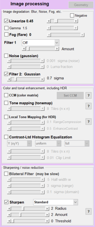Image Processing controls

Nonlinear functions should be avoided because they do not give reliable results.

These include Tone mapping, Local Tone Mapping, Contrast-Ltd Histogram Eq, and Bilateral Filter. In the process of writing the EI2024 paper, we discovered that USM (Unsharp Masking) sharpening is not linear. There was no indication of this in the MATLAB documentation. We discuss USM nonlinearity in the Image Processing page and in Interpolated slanted-edge SFR (MTF) calculation.

Applying image processing

We are most interested in the combined effects of lowpass filtering and sharpening.

To apply image processing to an image file,

Open Image Processing. The window shown below appears. Image Processing instructions contains more detail.

Image Processing opening window

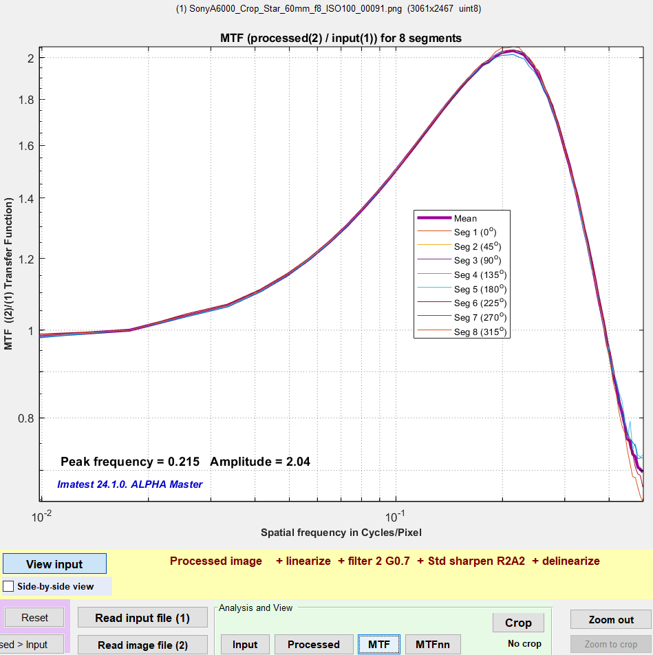
Image Processing transfer function for standard sharpening with R = 2, A = 2, G = 0.7.

Read the file by pressing Read input file (1).
Set the image processing. A typical example is shown above. Linearize, Filter 2, and Sharpen are checked. The file will be linearized assuming an encoding gamma of 0.45, blurred with a gaussian filter with σ = 0.7 pixels, sharpened (standard) with R = 2, A = 2, then re-gamma-encoded to gamma = 0.45.
Press Update calculations. Details on viewing the results are in the Image Processing instructions. We show a small version of the transfer function (MTF) on the right. Click on it to view full-sized.
To save the processed file, press Save image file (2).

In running several images, starting with a reasonably sharp raw-converted image, we found that moderate lowpass filtering (LPF), helped; LPF with moderate sharpening gave similar results (but could be less susceptible to interference from neighbors), but strong sharpening without LPF degraded the Edge SNRi.

Results

Quick summary of results: the mildly sharpened + LPF result is similar to the filtered result. But the strongly sharpened result shows some degradation (about 2dB). Click on the images to view full-sized.

Unprocessed (no ISP)

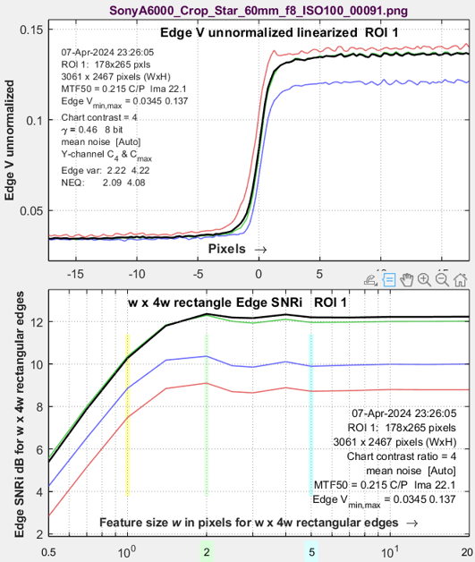Lowpass-filtered (LPF) σ=0.7

Slight improvement

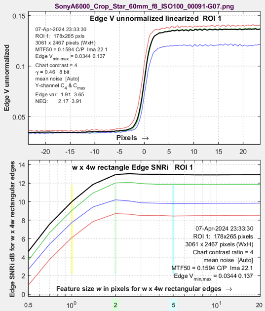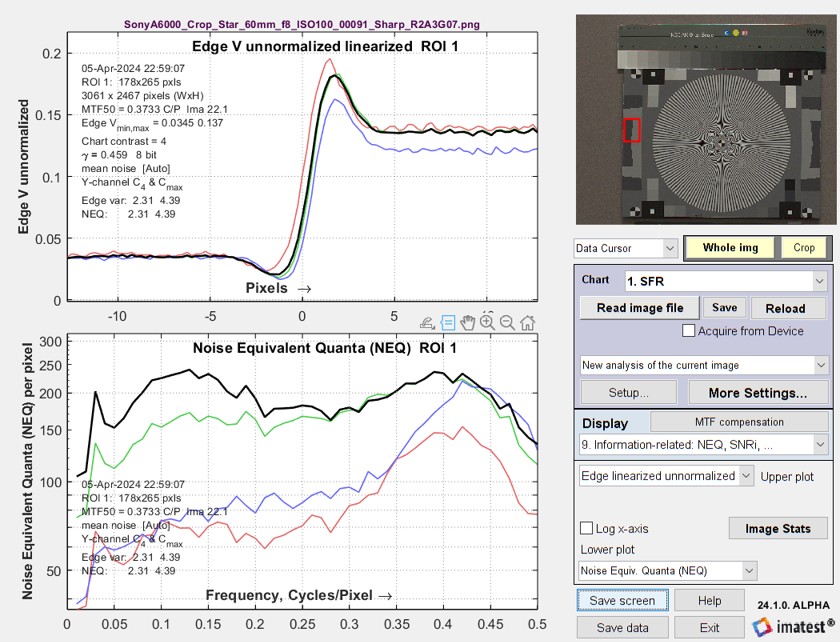
Sharpened + LPF R=2 A=1 σ=0.7

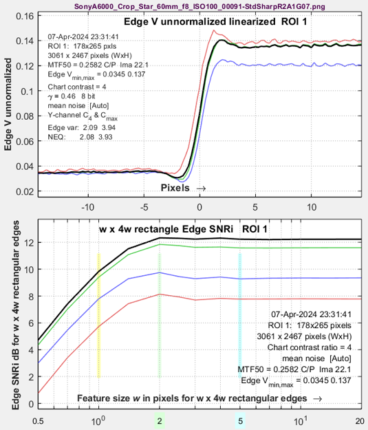Strongly sharpened R=2 A=3

Definite degradation

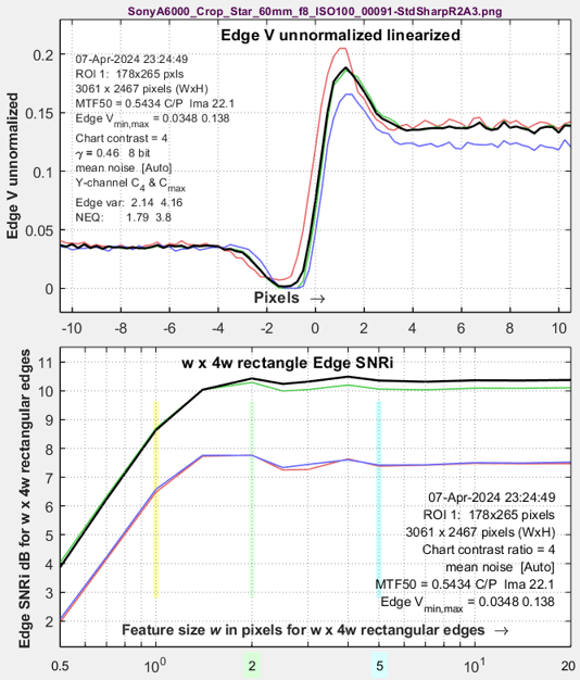Appendix: The problem with Unsharp Mask (USM)

According to the theory presented in the Electronic Imaging 2024 paper, linear, uniform, and reversible image processing should have an identical effect on SFR²(f) and NPS(f), where NPS(f) is the Noise Power Spectrum, and hence should not affect Noise Equivalent Quanta, \(NEQ(f)=\mu\ SFR^2(f) / NPS(f)=\mu\ K(f)\), where “reversible” means no response nulls below the Nyquist frequency (0.5 C/P). But we found inconsistencies in NEQ(f) when we applied Unsharp Mask (USM) sharpening (the MATLAB imsharpen function). We expected imsharpen to be linear, but we eventually found out that it was not. The nonlinearity is omitted in the MATLAB documentation.

Results for an unprocessed image and images processed with USM and linear sharpening are shown below.

No image processing.

Sony A6000. Straight out of LibRaw, unsharpened, NEQ is in the bottom plot.

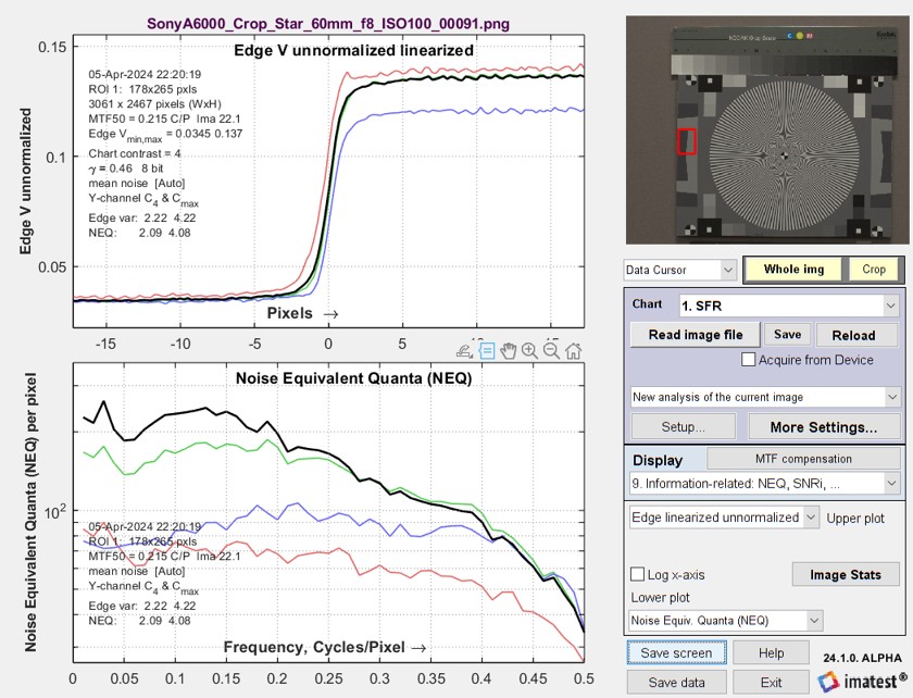USM R2A3 Gaussian 0.7.

The Sony A6000 image (above) has been filtered with a σ = 0.7 Gaussian Lowpass filter and an R2A3 USM sharpening, obtained with the Imatest Image Processing module.

Check Filter 2 Gaussian, and set sigma (0.7 pixels in this case) with the slider.
Check Sharpen, select USM (Unsharp Mask), and in the sliders, and set Radius and Amount (2 and 3 in this case).

NEQ(f) is very different from the unsharpened image: it is strongly boosted between 0.3 and 0.5 C/P. But we expected it to be nearly identical (for linear image processing). This discrepancy caused us a lot of grief in early 2024. Because we finally started to suspect that the MATLAB Unsharp Mask (USM) implementation (the imsharpen function) caused the problem, we developed a standard linear sharpening algorithm (a 2D version of the 1D sharpening described in the Sharpening page). We knew it was linear because we wrote the code.

Standard sharpening
(a new addition to Image Processing).

This is a 2D extension of the 1D sharpening algorithm described on the Sharpening page. The steps to create this in Image Processing were

Check Linearize and use the slider to the right to set to the encoding gamma (to be removed by linearization) to 0.45. This encoding gamma will be restored when the calculations are complete.
Check Filter 2 Gaussian, and set sigma (0.7 pixels in this case) with the slider.
Check Sharpen, select Standard in the adjacent dropdown menu, and set Radius and Amount (2 and 3 in this case) in the nearby sliders. Standard sharpen is a 2D version of the 1D sharpening described in the Sharpening page. It was developed by Imatest, and it contains no nonlinear processing.
Detailed description in the Image Processing page.

NEQ is nearly identical to the unsharpened image, as expected. This result was a huge relief. It confirmed that Imatest calculations are consistent as long as image processing is linear.

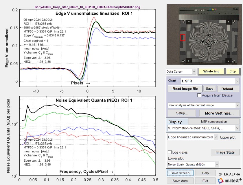The cause of the NEQ inconsistency was the nonlinearity of MATLAB’s USM processing,
not a deficiency of the binning algorithm.

This is why we recommend Standard sharpening (which should be used with the Linearize function),
and not USM.

News

Knowledge Base