Introduction – The problem and its solution – working with the interpolated algorithm – Identifying the problem –
Image comparisons – Algorithm – SFRMAT5 – Extreme noise – Motion blur – Summary
Introduction
Note: MTF (Modulation Transfer Function) and SFR (Spatial Frequency Response) are (almost) synonymous. Older papers mostly use MTF, but the current practice (for example in recent versions of the ISO 12233 standard) prefers SFR.
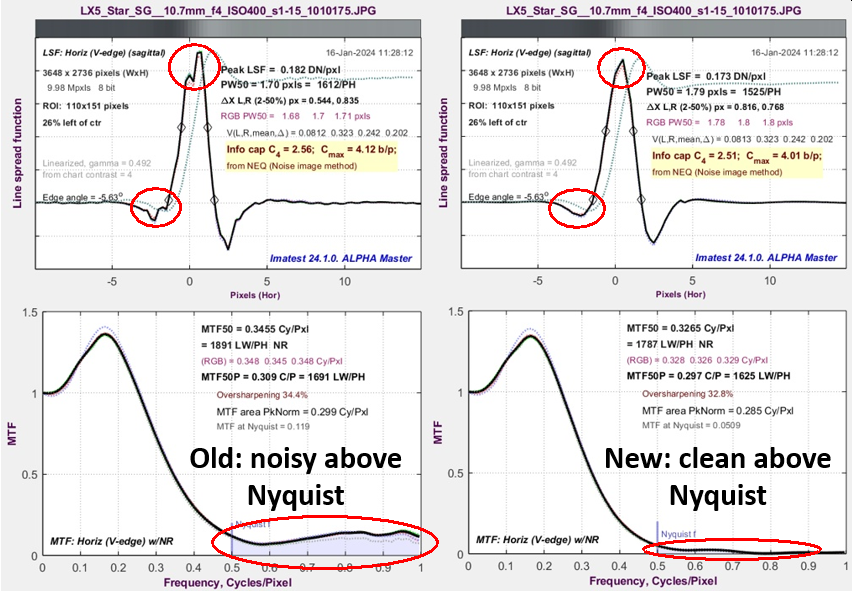
Old vs. Interpolated: Line Spread Function (LSF) and MTF (SFR)
In the process of developing the image information metric calculations, we observed an inconsistency in the Noise Equivalent Quanta (NEQ) calculations, which should be unaffected by image processing as long as it is linear and uniform.
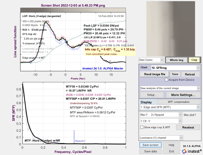
We also observed artifacts at high spatial frequencies (shown on the right) that we thought might have been related to the inconsistency. The artifacts were greatly reduced when the interpolated binning algorithm, described below, was applied.
As long as simple metrics like MTF50 were sufficient, the high frequency artifacts could usually be ignored. But we had to address them because we were concerned about their effect on the image information metrics, most of which are derived from the calculation kernel, \(K(f) = SFR^2(f) / NPS(f)\), where NPS(f) is the Noise Power Spectrum.
According to the theory presented in the Electronic Imaging 2024 paper, linear, uniform, and reversible image processing should have an identical effect on SFR2(f) and NPS(f), and hence should not affect Noise Equivalent Quanta, \(NEQ(f)=\mu\ SFR^2(f) / NPS(f)=\mu\ K(f)\), where “reversible” means no response nulls below the Nyquist frequency (0.5 C/P). But we found inconsistencies in NEQ(f) when we applied Unsharp Mask (USM) sharpening (the MATLAB imsharpen function). We expected imsharpen to be linear, but we eventually found out that it was not. The nonlinearity is omitted in the MATLAB documentation.
This document describes the development of the interpolated binning algorithm, the results of a number of tests, and why it failed to solve the inconsistency.
The problem and its solution
This section contains recent results (April 2024). A description of the interpolated binning algorithm and earlier results follow.
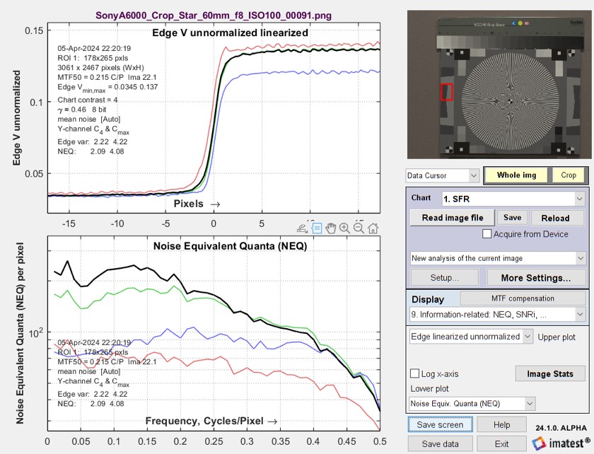
No image processing.Sony A6000. Straight out of LibRaw, unsharpened, NEQ is in the bottom plot. |
 |
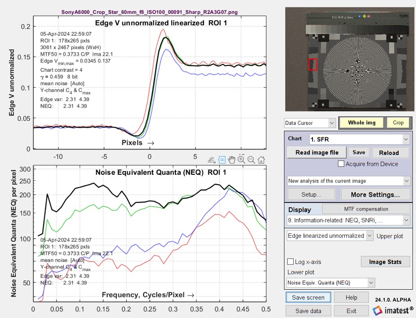
USM R2A3 Gaussian 0.7.The Sony A6000 image (above) has been filtered with a σ = 0.7 Gaussian Lowpass filter and an R2A3 USM sharpening, obtained with the Imatest Image Processing module.
NEQ is very different from the unsharpened image: it is strongly boosted between 0.3 and 0.5 C/P. But we expected it to be nearly identical (for linear image processing). This discrepancy caused us a lot of grief in early 2014. Because we finally started to suspect that the MATLAB Unsharp Mask (USM) implementation (the imsharpen function) caused the problem, we developed the standard sharpening algorithm (a 2D version of the 1D sharpening described in the Sharpening page) that we knew had to be linear because we wrote the code. |
 |
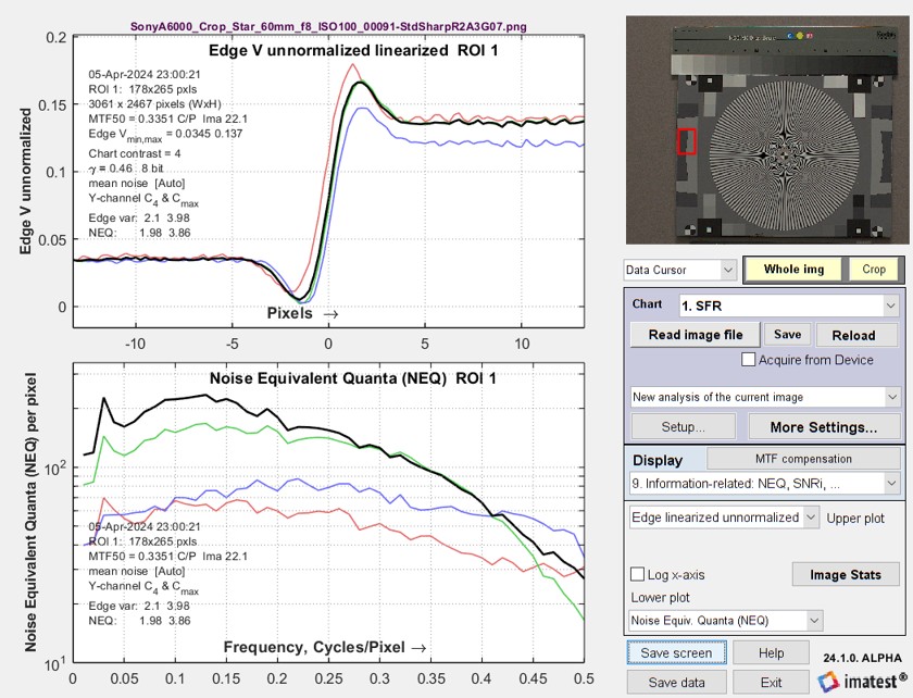
Standard sharpening
|
 |
|
The cause of the NEQ inconsistency was the nonlinearity of MATLAB’s USM processing, (The pesky high frequency artifacts appear to be the result of demosaicing.) The remainder of this page is primarily archival material, |
Working with the interpolated algorithm
| Before we found the cause of the problem we spent quite a lot of time developing the interpolated binning algorithm and working with it. Although it didn’t solve the calculation consistency problem, it effectively removed the high frequency artifacts. We found some uses for it, but we can’t recommend it for general use. The documentation that follows is an archive. |
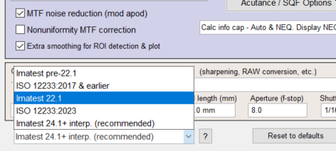
When we developed Imatest 24.1, we attempted to remedy the NEQ calculation inconsistency with an interpolated binning algorithm that fixed the high frequency SFR artifacts present in standard ISO 12233-based algorithms. Interpolated binning can be selected in the dropdown menu that selects the binning algorithm, located on the lower-left of the SFR Settings or More Settings windows.
As we gained experience with the interpolated binning calculation, we realized that interpolation method has a frequency response of sinc2(fT) for sampling interval T, and that much of the reduction of high frequency artifacts can be attributed to this rolloff. However, the improvement in the line spread function in Motion blur, below, is still significant. (We don’t have another way of removing the zigzag artifacts.) And results are very consistent with Siemens star calculations. We now believe that the artifacts are caused by demosaicing. We’ve observed that they can be very different in JPEGs from cameras and raw images converted with LibRaw. Generally worse in camera JPEGs (for reasons unrelated to JPEG compression).
Identifying the problem (the calculation inconsistency)
|
The work was motivated by an inconsistency we observed with the Noise Equivalent Quanta (NEQ) measurement, which is one of the new image information metrics. NEQ should not be affected by uniform, linear filtering— sharpening or lowpass filtering, but we found significant variations. We were able to determine that the noise spectrum was consistent. The two plots below show NEQ for the same image capture with different filtering. Left: lowpass-only. Right: strong sharpening with lowpass. Note that the y-axis scales are very different. These results are confusing and ambiguous, but along with other measurements they were a cause of concern. Note: processing with a gaussian = 0.8 pixel LPF is problematic. It seems to cause the null around 0.43 C/P. In later work we switched to 0.7 for improved reversibility. |
|
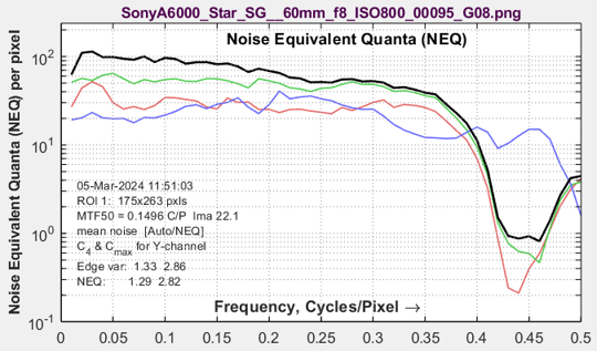 NEQ for gaussian = 0.8 pixel LPF Note that NEQ for the luminance channel drops to half its peak value around 0.3 C/P. (Disturbing observation: the individual color channels do not drop as much.) |
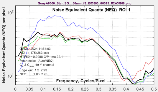 NEQ for USM R2A3 (strong sharpening) + gaussian = 0.8 pixel LPF Note that NEQ for the luminance channel drops very little from its peak value to around 0.3 C/P. |
|
The problem or high frequency artifacts was identified and a partial solution was presented in the 2017 paper, Reverse-Projection Method for Measuring Camera MTF, by Stan Birchfield. In Figure 8 from the paper, shown on the right, the ISO-based results all have higher SFR and rough response at high frequencies (above 0.65 Cycles/Pixel). The reverse-projected results are very well behaved (have little response) at high frequencies. |
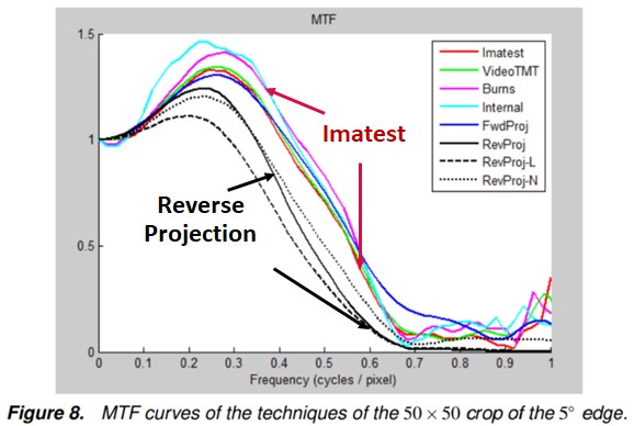 |
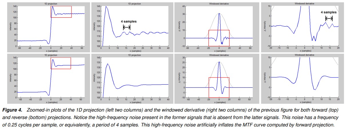
Figure 4 from Birchfield’s paper shows details from an ISO-based calculation (which includes Imatest) on the top and the new reverse-projected calculation (on the bottom).
Results are strikingly similar to old and new Imatest results. We chose not to use Birchfield’s technique for three reasons. 1. It appears that it will be difficult to adapt to curved edges, i.e., images with optical distortion. 2. It is protected by U.S. Patent 10,429,271, assigned to Microsoft. 3. It required only a few lines of code to fix the issue with the old ISO 12233-based calculation. In addition, it appears to have a comparable high frequency rolloff (sinc2(fT)) to our interpolated method: response is significantly reduced at the Nyquist frequency, compared to the standard ISO calculation.
Image comparisons for compact digital camera at ISO 400
|
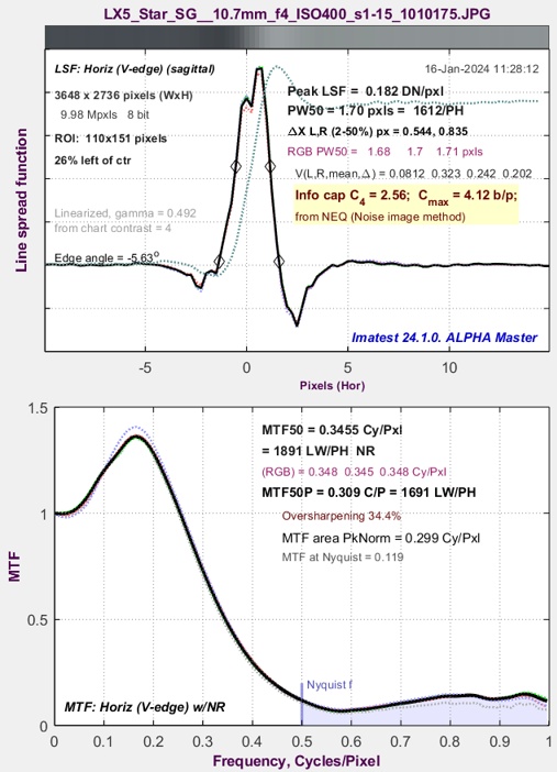
Old Imatest (ISO-based) slanted-edge calculation |
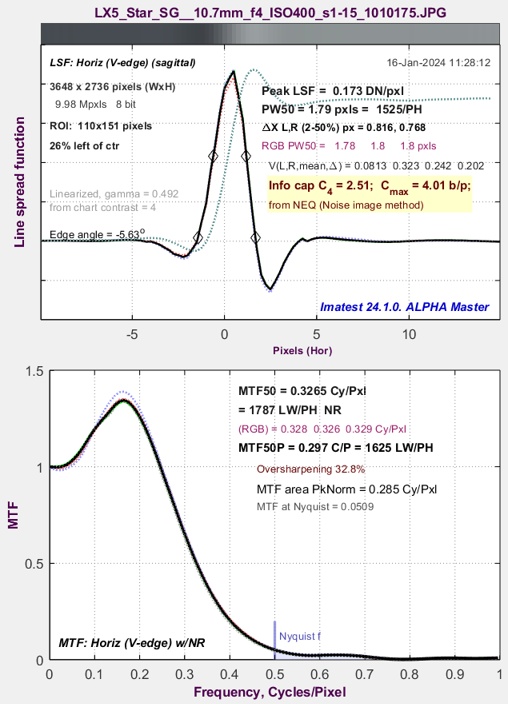
Imatest 24.1+ interpolated slanted-edge calculation |
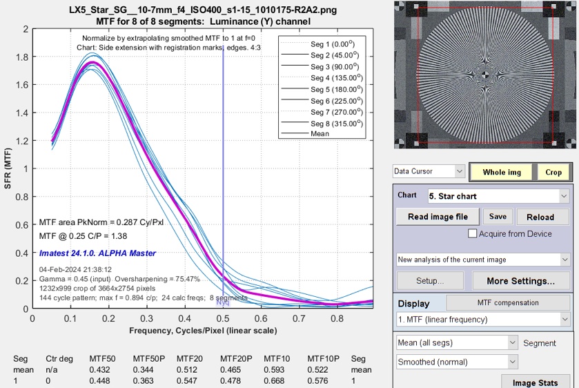
The JPEG image file for these results (2.07 MB) can be found here. 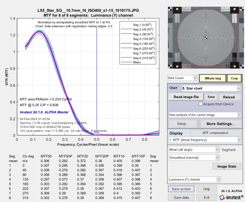 Siemens star SFR (MTF) from same (LX5 ISO 400 JPEG) image,
which appears to have a moderate amount of bilateral filtering. Mean MTF50P = 0.282 C/P.
The Siemens star SFR has been normalized by extrapolating the smoothed SFR curve to 1.0 at zero frequency. This is realistic method for normalizing strongly sharpened images for the star, which doesn’t go to low spatial frequencies, and it helps to match the results with slanted edges.
This image appears to have some bilateral filtering (sharpening near the edge; noise reduction elsewhere), indicated by a noise peak near the transition. This can cause some difference between the slanted-edge and Siemens star results. But the difference is small.
|
Edge noise for the JPEG image, above. |
Edge noise for the USM-sharpened PNG image, below. |
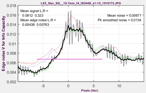
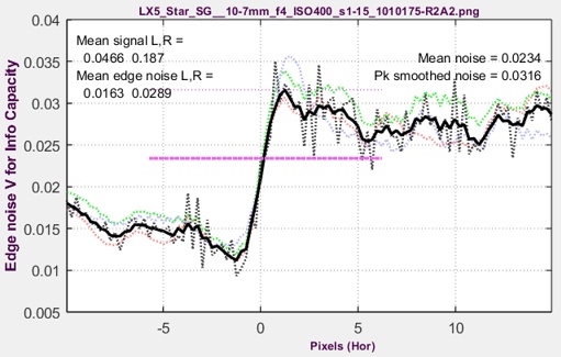
The Siemens star result is slightly different from the new slanted-edge result because the image is a JPEG from a camera, which has some bilateral filtering (which tends to affect edges more than sines). However it’s not very different.
| It’s time to dispel the myth that slanted-edges are affected by bilateral filter sharpening, but Siemens stars are not. They are both affected, though the slanted edge may be more strongly affected. One reason: the ISO standard slanted edge has a 4:1 contrast ratio. It’s 50:1 for the standard star (though lower contrast stars are available). |
II. RAW→TIFF→USM-sharpened PNG (R2A2)
Uniformly sharpened with USM, Radius = 2, Amount = 2 (R2A2)
When an image is uniformly sharpened, the slanted-edge and Siemens star results are extremely close. This was never the case with the old ISO calculation.
|
|
|
Siemens star SFR (MTF) from same (LX5 ISO 400 RAW→TIFF→PNG, USM R2A2-sharpened) image,
Mean MTF50P = 0.344 C/P.
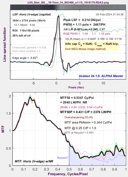
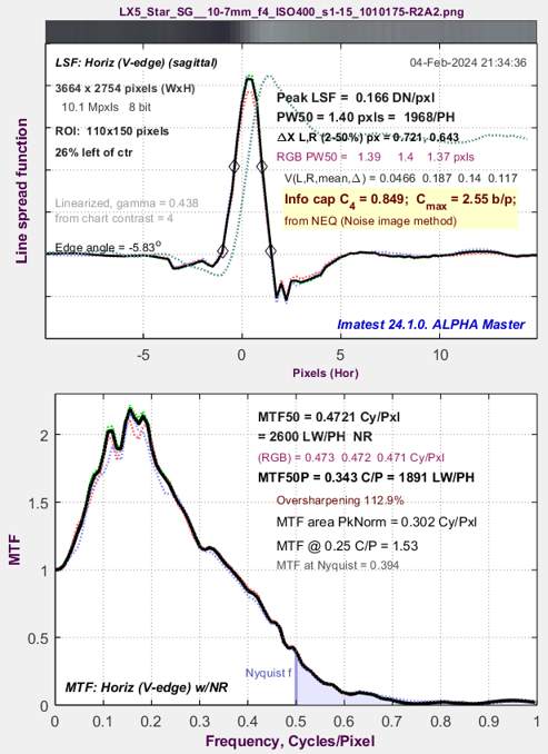
The old slanted-edge calculation is very noisy— very ugly— so bad that the information capacity calculation fails. MTF50P is virtually identical for the new interpolated calculation and the Siemens star— no, we didn’t cherry-pick the image. MTF50 is very close, but not identical. The shapes of the SFR curves are also close but not identical: the slanted-edge has more response at Nyquist (fNyq = 0.5 C/P).
|
The slanted-edge calculation method is selected on the lower-left of the Settings window for SFR or the More settings window for Rescharts slanted-edge modules. To run the new interpolated calculation, select Imatest 24.1+ interp. Note that Imatest 22.1 (the old method) is still recommended. |
 |
Algorithm
The key to the algorithm was the realization that the image had to be interpolated to give good results. No matter what we did with an uninterpolated image, the same problems (sawtooth noise and irregular response above the Nyquist frequency) persisted. And we noticed that interpolation was an integral part of the reverse-projection algorithm.
The algorithm follows the ISO 12233 standard with just the addition of interpolation. Here is a brief summary of the ISO algorithm.
- Linearize the image using the inverse of the measured gamma curve or the edge itself, if the contrast is known.
- Find the center of the transition for each horizontal scan line.
- Fit a polynomial curve to the center locations of the scan lines.
- Add each horizontal scan line to one of four bins, based on a polynomial location at each scan line.
- Combine the bins to obtain a 4x oversampled interleaved average edge, which is used to calculate SFR. This effectively applies signal averaging, which improves SNR by the square root of the vertical ROI height/4.
The interpolation is applied between steps 3 and 4, so that horizontal scan line pixel count is increased from Nwid to 2×Nwid+1 pixels.
Interpolate the columns of an Nwid (width) × Nht (height) image, so that the size becomes 2×Nwid-1 × Nht pixels. Each pixel in the yellow vertical bars shown below (each representing a column of pixels) will contain data interpolated from the pixels to the left and right. The MATLAB interp2 function was used to perform the interpolation. We preferred the ‘cubic’ method, although ‘linear’ wsn’t very different and would have been somewhat faster. The polynomial curve (fit to the centers of the scan lines) is adjusted for the interpolation.
 Here are examples of input and interpolated image data.
 Original image |
 Interpolated image Interpolated image |
The interpolated data is binned using the same procedure as the standard uninterpolated method. But there are almost twice as many points in the horizontal scan lines (2×Nwid-1 vs. Nwid). Based on the above results, it makes a remarkable difference.
SFRMAT5
The free SFRMAT5 program, available from Peter Burns (Burns Digital Imaging) is used as the platform for example code required by the ISO 12233 committee. We have added the new interpolation code to a version of SFRMAT5 and communicated it to Peter, but we haven’t determined how it will be distributed. Here are results from SFRMAT5 without and with the new interpolation method.
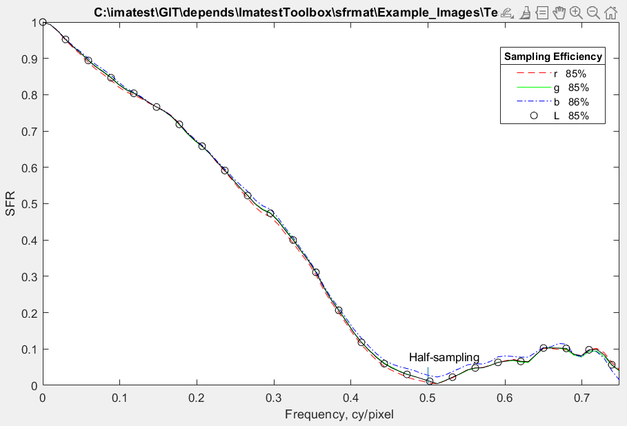 SFRMAT sample edge results SFRMAT sample edge resultsold method: no interpolation |
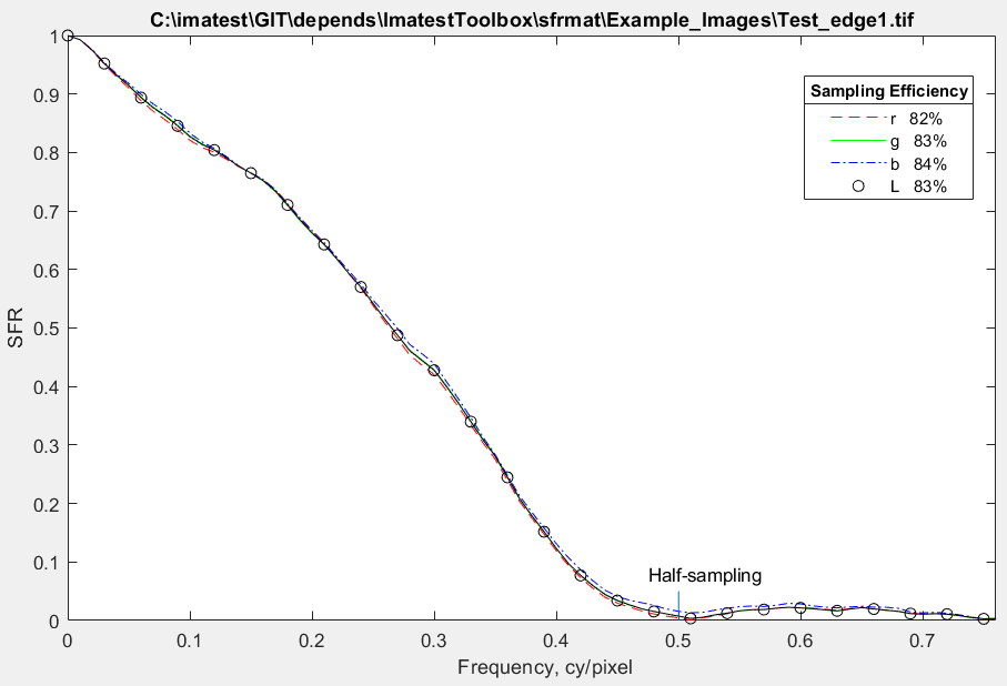 SFRMAT sample image results SFRMAT sample image resultsNew method: interpolated |
We will use SFRMAT5 as the platform for sample code for the ISO 23654 standard for information-related metrics.
More examples
Extremely noisy image
Here is a dramatic example of an extremely noisy image: a TIFF from the Micro Four-Thirds Sony A6000 acquired at ISO 12800.
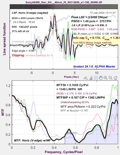 Old method Old method |
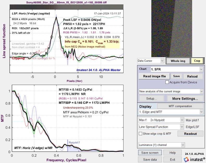 Interpolated (new) method Interpolated (new) method |
The large TIFF image used for the above results has been cropped and saved as a JPEG, with no changes in image processing.
The image file (3.92 MB) can be found here.
I tried to quantify motion blur using the Line Spread Function with the old calculation, but sawtooth artifacts (visible on the left, below) spoiled the calculation.
Here are two downloadable images (motion blur on the right) and results before and after the fix. I don’t remember if the blur was real or simulated. It would make no difference.
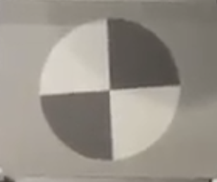 No motion blur No motion blur |
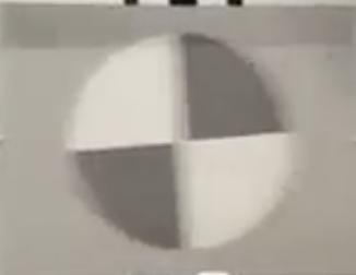 Motion-blurred Motion-blurred |
Looking at the top vertical edge of the blurred edge on the right,
|
|
|
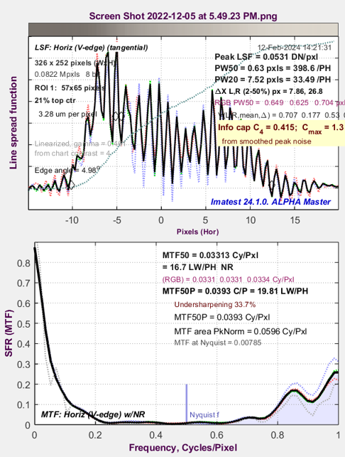
This shows a clear and unambiguous improvement for the new interpolated binning algorithm, and is the primary reason we are keeping it.
Design and Measured MTF Transfer functions
A. Gaussian 0.8
 Gaussian 0.8 LPF: design Gaussian 0.8 LPF: design |
USM sharpen Radius 2 Amount 5 (R2A5), Gaussian 0.8
 |
(incomplete. Details coming soon.)
Summary
- Fewer high frequency noise-like artifacts
- Better agreement with Siemens star results
- Suppression of sawtooth (or zigzag) artifacts, that were particularly troubling when I was looking at the Line Spread Function with motion blur.
On the other hand, there are some concerns about the interpolation method
- Definitely has a high frequency rolloff. Apparently it is sinc2(fT) for sampling interval T, which has affects MTF measurements.
- The HF rolloff was significant for some reference edges with very short rise distance. MTF at 2*Nyquist was lower than expected.
- The high frequency artifacts removed by interpolated binning may be real phenomena caused by demosaicing. It tends to be different in JPEGs from cameras and images converted from raw offline, then sharpened equivalently to the JPEGs (and the difference appears to be unrelated to JPEG compression).
|
The bottom line Although the interpolated binning method is of some interest — it fixed the zigzag issue in motion blur images and provides better agreement with Siemens star results — the earlier (22.1) binning method remains our recommendation for most calculations. |
- Why is agreement with the Siemens star so good?
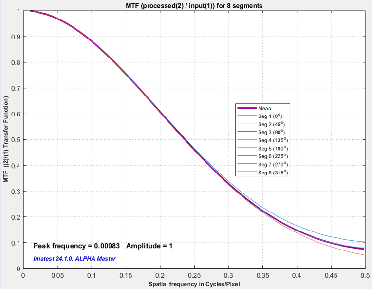
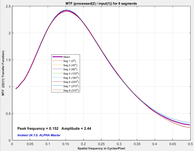
- Here is the problem I observed that got me into this rabbit hole: I can observe transfer functions between images with different filtering. It is particularly interesting to look at the transfer function of sharpened vs. unfiltered images. With small to moderate amounts of sharpening, results are as expected. With large amounts of sharpening (very large overshoot), the MTF is exaggerated: the peak is much larger than expected. This caused the inconsistency in NEQ measurements that I found upsetting. I had to conclude that (A) results with extreme sharpening are not valid, but they’re not important because we will never sharpen this much. (SNRi was too good). (B) I don’t know the cause of the issue. Could be related to aliasing.
- Does demosaicing affect the frequency response of edges differently from noise (where it acts like interpolation– it’s a lowpass filter).