|
Imatest InfoDR (Information-based Dynamic Range) refers to an Imatest module and a set of test charts designed to measure C4 information capacity over a wide range of illumination — This page, Part 1, describes the InfoDR charts and how to photograph them. |
Part 1 – Introduction – C4 Information Capacity – InfoDR chart versions – Lighting – Measuring illumination
Photograph (framing) – Appendix: InfoDR chart design
Part 2 – Open, Select, & Read – Setup window – Results – Information-related displays – More settings
Introduction
|
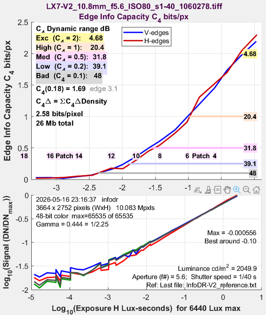
Imatest InfoDR (Information-based Dynamic Range) is a Rescharts module and a set of accompanying test charts designed to measure Dynamic Range and camera performance over a wide range of illumination, based on C4 information capacity (information capacity measured directly from 4:1 contrast ratio slanted edges). Unlike the SFRplus, eSFR ISO, and Checkerboard charts, which are designed to fill most of the image). the InfoDR charts are designed to occupy only the central portion of the image. Region of Interest (ROI) selection is automatic. Low-light and Dynamic Range measurements are far more accurate than traditional charts because the signal is the edge contrast— the difference between adjacent patches— and hence does not reward stray light with better measurements. The curve on the right plots C4 information capacity as a function of sensor illumination. The area under the curve, C4 Δ = ∑C4ΔD (for density increment, ΔD = 0.2 for the two-layer film chart), is a preliminary heuristic figure of merit, combining C4 and dynamic range. |
 |
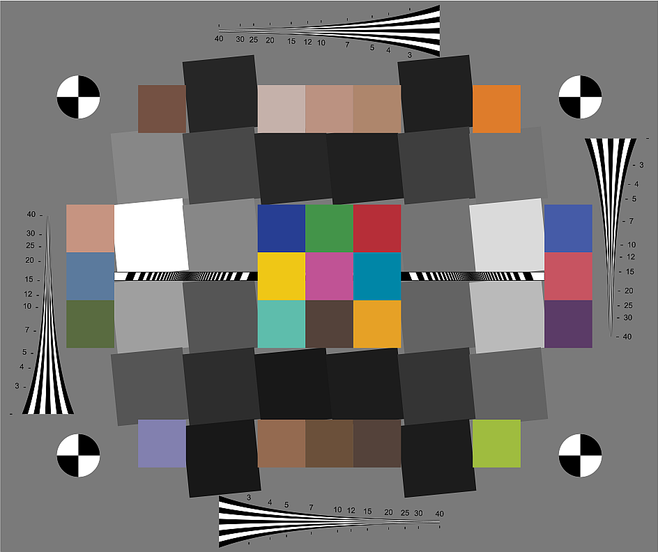
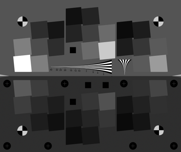
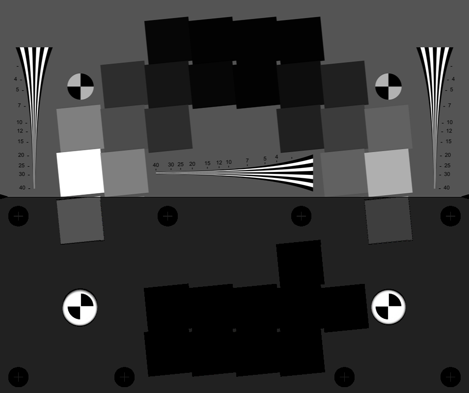
Example of InfoDR chart (single layer transmissive)
InfoDR test charts consist of a compact arrangement of slanted squares, divided into four quadrants or six regions, where adjacent squares within each quadrant or region has a constant density ratio of 4:1, or equivalently, an Optical Density difference ΔOD = 0.6. The patch densities in each region are offset so the patches have constant density steps over the chart as a whole. The chart also has added features (color patches and wedges) of value to customers for camera testing. The principles behind the chart design is described in the Appendix, below.
InfoDR charts are primarily intended to be analyzed as a part of Imatest Rescharts, but they can also be analyzed with Color/Tone (Interactive and Auto), which, however, only calculates traditional SNR-based metrics, including Dynamic Range.
InfoDR test charts may be purchased from the Imatest store (recommended) or printed on a high-quality inkjet printer (reflective version-only).
InfoDR Image quality factors
Primary result
 C4 information capacity (information capacity measured directly from a 4:1 contrast edge), measured over a wide range of illumination, including low light. Derived from sharpness and SNR, where the signal S is the difference between the levels on either side of the slanted edge. A superior metric for low-light performance.
C4 information capacity vs. luminance (cd/m2)
This is a key result of InfoDR.
Other important results
- Sharpness, expressed as Spatial Frequency Response (SFR), also known as Modulation Transfer Function (MTF)
- Noise and Signal-to-Noise Ratio (SNR), measured from the grayscale patches surrounding the center of the chart, includes all types of noise calculated by Color/Tone Interactive and Color/Tone Auto (standard pixel noise, chroma noise, scene-referenced noise, sensor (raw) noise, and ISO-15739 visual noise and dynamic range). SNR (Signal-to-Noise Ratio) can also be displayed as a ratio or in dB.
- Tonal response (also from the grayscale patches).
Additional (secondary) results
- Lateral Chromatic Aberration (LCA) Can be displayed, but is not generally useful because the InfoDR chart normally covers only the central portion of the image field. LCA is most significant near the edges of the image.
- Color accuracy, only available on reflective (usually inkjet) or single-layer transmissive (LVT color film) versions of the InfoDR chart (not the two-layer transmissive versions for measuring Dynamic Range).
- ISO sensitivity (Saturation-based and Standard Output Sensitivity), when illuminance (candelas/meter2) is entered.
- Onset of aliasing and Moiré, measured from the four pairs of wedges in the Enhanced and Extended charts, whose spatial frequency range is the same as the separate ISO 12233:2017 wedge chart. Figures and results are identical to the Wedge module.
C4 Information capacity
C4 is the information capacity of a pixel or the total image for an object with a contrast ratio of 4:1 (an optical density difference of ΔD = 0.6) relative to the background. it is typically measured in units of information bits per pixel or image. C4 is measured directly from 4:1 contrast slanted edges, as specified in the ISO 12233 standard, with some enhancements to make them more precise and repeatable.
C4 is a measure of the amount of information can be contained in a 4:1 contrast signal.
Why information capacity?
The most important of the traditional measurements are sharpness, usually expressed as MTF (Modulation Transfer Function) or SFR (Spatial Frequency Response), which are synonymous is practice, and noise or Signal-to-Noise Ratio (SNR). Other measurements, such as distortion, tonal response, and color quality are fully or partially correctable, and are not directly related to the amount of information in an image.
|
Information capacity C4 is a more fundamental measure of image quality than either sharpness or noise, \(\displaystyle C = \int^B_0{\log_2\left(1+\frac{S_{avg}(f)}{N(f)}\right)}df \) for bandwidth B = fNyquist = 0.5 C/P, mean signal power, Savg(f) = (AP-P/12 MTF(f))2 for
|
The frequency-domain representations of signal and noise power are derived from spatial measurements of the slanted edge, which are summarized in Image Information Metrics. This page also contains numerous links to the image information metrics documentation. A full description of the calculations and metrics can be found in the revised Electronic Imaging Conference 2024 paper, “Image information metrics from slanted edges.“.
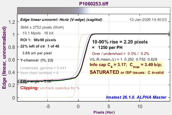
Saturated edge (the lightest edge in the example image on this page). Noise is zero in the saturated region.
Why 4:1 contrast ratio?
The original ISO 12233 standard called for a minimum of 50:1 contrast, but it was discovered that 50:1 contrast was too high to produce reliable results because the image would often saturate, i.e., reach its maximum allowable level (typically 255 for 8-bit files or 65535 for 16-bit files), creating a sharp corner at the onset of saturation that erroneously boosted high frequency components and hence MTF. 10:1 was appealing because it looked a lot like 50:1, but it was still a little too susceptible to saturation. 4:1 was a compromise — and in our experience remains an excellent compromise. Among its attributes.
- Most real-world objects that need to be recognized are not extremely high contrast.
- System operation is linear for 4:1 contrast objects in well-exposed images (when the image is linearized, i.e., gamma-encoding is removed). Because of this linearity, performance at other contrast levels, for example 2:1, where low SNR would make measurements difficult, can be estimated reliably.
Effects of stray light on SNR measurement
There is an important difference between the signal used to calculate the SNR in conventional and in information-based measurements.
- For conventional measurements, the signal s is simply the patch level. But stray light increases this level in dark regions, while fogging detail. This causes the SNR measurement to increase while performance is degraded, i.e., measurements in dark areas are inaccurate when stray light is present. This effect can be mitigated somewhat by dividing the noise by the slope of the signal as a function of illumination, as is done in scene-referenced noise calculations.
- For C4 measurements, the signal s is the difference between the light and dark levels adjacent to the edge. Stray light does not cause a measurement error. Measurements are accurate and robust.
Focus
Another important difference between C4 and standard SNR and Dynamic Range measurements is that C4 measurements must be in good focus. Focus doesn’t matter for traditional SNR measurements, where noise is the standard deviation of the digital numbers in the patch (with some compensation for nonuniform illumination). Because of the focus requirement, there may be instances where large charts, such as VisNIR charts, which can be printed up to 28×32 inches, and are compatible with large Fields of View since the chart isn’t designed to fill the field, may be needed. There may even be cases where collimators are required.
HDR (High Dynamic Range) sensors
HDR sensors have several operating regions, defined by discontinuities (steps in noise) in the operating curve, i.e., the operating curve is different from standard linear sensors. As a result, the total information capacity, Cmax, which involves extrapolating the noise, cannot be measured reliably. However C4, which is measured directly and doesn’t involve any assumptions, can be measured reliably for HDR sensors.
Algorithm for measuring MTF and C4 in the darkest regions
InfoDR charts, especially transmissive versions, include very dark (high density) patches, where the SNR may become so low that MTF cannot be reliably calculated. But the compact design of the chart, which is intended to keep MTF relatively constant throughout the active area of the chart, allows us to perform a trick to obtain reasonable values of MTF, and hence C4, in the darkest regions.
Although, patches are numbered in row-major order from top to bottom to facilitate patch density measurements, edge numbers, and hence MTF calculations, are sequenced from light to dark (there is an example in the Appendix). MTF calculations are reliable for the brighter patches (except when a patch is saturated), but become unreliable for the darkest patches. To remedy this problem, we save the last “good” MTF measurement to use for the darkest patches. For now, we define the “last good measurement” as the last MTF measurement where the sum (or integral) of MTF between f = 0 and f = fNyquist (the Nyquist frequency = 0.5 C/P) is greater than the sum of MTF between fNyquist and 2×fNyquist. This MTF measurement is “good enough” because C4 tends to be extremely low (often below 0.2 bits per pixel), i.e., practically nonexistent, for the darkest patches.
InfoDR Chart versions
The two-layer transmissive charts, which have sufficient tonal range to measure dynamic range on most cameras, are likely to be more popular versions. Transmissive charts are supplied with individually-measured density files in CSV format (or CIELAB (L*a*b*) reference files for the version with color patches) because they can’t be produced as consistently as reflective files (usually made on inkjet media).
| Chart type Attribute |
Reflective (inkjet) |
Transmissive 1-layer (LVT film) |
Transmissive 2-layer (LVT file) |
VisNIR 2-layer Photomask |
| Number of patches/edges | 24/24 | 28/32 | 42/48 | 40/48 |
| Patch density range | 2.25 (45 dB) | 2.85 (57 dB) | 5.2 (104 dB) | 7.5 (150 dB) |
| Edge density range (Note [1]) | 1.65 (33 dB) | 2.25 (45 dB) | 4.6 (92 dB) | 6.9 (138 dB) |
| Number of patches/edges | 24/24 | 28/32 | 42/48 | 40/48 |
| Edge Density step ΔD | 0.15 | 0.15 | 0.2 | 0.3 |
| Spectrally neutral | ♦ | Note [2] | ♦ | |
| Maximum size (Note [3]) | 44×52.5 in; 112×133 cm total | 9.25×7.75 in; 23.5×19.7 cm active (8×10 in. total) | 9.25×7.75 in; 23.5×19.7 cm active (8×10 in. total) | 26.8×32 in; 68×81 cm total |
| Summary | Easy to print on inkjet media, but insufficient density range for most cameras. | Better density range then reflective, but still insufficient for most cameras. | Sufficient density range for most cameras. Visible light-only. Limited size. | Sufficient density range for extreme HDR cameras. Can be printed much larger than LVT film. Response to LWIR. Spectrally neutral. Ultrafine halftone pattern. |
Notes
- Since there are two edges for each density increment, ΔD, Edge density range = (Nedges/2-1)ΔD.
- Slight tinting of film patches has little effect on measurements; it’s more of a cosmetic issue.
- Based on Aspect Ratio = 9.25:7.75 (maximum size of active area on 8×10 inch LVT film)
LightingTransmissive charts should be backlit using a lightbox or panel, several of which are available on the Imatest Store. Reflective charts — The chart on the right summarizes lighting considerations. The goal is even, glare-free illumination. Lighting angles between 20 and 45 degrees are ideal in most cases. At least two lights (one on each side) is recommended; four or six may be better. Avoid lighting behind the camera, which can cause glare. Check for glare and lighting uniformity before you expose. Lighting systems can be found on the Imatest Store. |
 Simplified lighting diagram |
Chart illumination
Most previous Imatest tonal response and dynamic range plots used relative exposure units for the independent (x) axis — f-stops or EV; (log2(e)), Optical Density (OD; log10(e)) or decibels (dB; 20×log10(e)), where e is relative exposure. But low light performance measurements require absolute illumination measurement. Two types of absolute illumination measurement must be distinguished. (They sometimes get confused.)
|
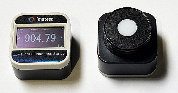
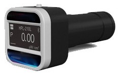
Illuminance — Light reaching an object (i.e., test chart), i.e., incident light in units of Lux (Lumens/meter2). Measured with incident light meters or illuminance meters. Only suited for reflective charts. The Imatest Low Light Illuminance Sensor (right) consists of two units connected by Bluetooth: the sensor unit (right) and the display unit (left). Measures Illuminance (Lux) between 0.1 and 200,000 Lux. To measure illuminance (incident light), the back of the sensor unit is typically placed in contact with the test chart surface, so the sensor element faces in the same direction as the test chart. |
 |
|
Luminance — light emitted from an object, either reflected from it or transmitted through it. Units of candelas/meter2 (cd/m2). This is what the camera actually “sees.” For Imatest measurements, the object is either a test chart or a lightbox. Luminance meters are designed to measure light emitted from an object, which can be either transmitted or reflected. They typically have optical systems that limit the angle of acceptance. For transmissive (backlit) charts they can be in contact with the chart or lightbox (the numbers are interpreted differently for these two cases). Reflective charts present challenges for luminance meters. They have be close enough to only read the patch of interest, but far enough to avoid shading the patch. For this reason, illuminance meters is preferred for reflective charts. |
|
For Lambertian surfaces (matte surfaces that reflect light equally in all directions) with reflectance ρ = reflected light/incident light,
Luminance (cd/m2) = L = ρE/π for illuminance E (Lux).
Plain white bond paper has reflectance ρ ≅ 0.92. Grayscale test charts are characterized by patch densities, D = -log10(ρ) or -log10(τ). A file containing measured patch densities, typically in CSV (Comma-Separated Variable) format, is supplied with Imatest transmissive charts (LVT film or VisNIR photomask).
Illuminance/Luminance equivalenceThe illuminance of a reflective chart in Lux can be considered equivalent to the luminance of a transmissive lighjtbox in cd/m2 if chart patches with the same density, D = -log10(ρ) or D = -log10(τ) for reflective or transmissive charts produce the same luminance. The equation is simple. Luminance L in cd/m2 = Illuminance E / π ; L = E/π or E = π L |
If you happen to have a meter reads in EV (Exposure Value): Lux=2.5×2(EV100) where EV100 = EV @ ISO 100, where EV @ ISO 100 is also known as Light Value (LV).
A key paper that explains illuminance and luminance, as well as the distinction between photometric units (which have spectral response similar to the human eye) and radiometric units (which have flat spectral response) is Radiometry and Photometry for Autonomous Vehicles and Machines – Fundamental Performance Limits by Robin Jenkin and Cheng Zhao, DOI : 10.2352/ISSN.2470-1173.2021.17.AVM-211 Strongly recommended
Traditional light meters, both incident and reflected, are designed for setting camera exposure (shutter speed and aperture) for a specified Exposure Index, commonly called “ISO speed”). Because such meters tend to be somewhat inaccurate, instruments specifically designed for measuring illuminance and luminance are recommended. We are adding a luminance meter to the Imatest Store.
Measuring chart illumination
Chart illumination should be measured for grayscale charts where results can be plotted as a function of absolute illumination level (generally chart luminance in cd/m2 or sensor exposure in lux-seconds). Good illumination measurements are more important for transmissive charts, which are used for dynamic range and low-light measurements.
|
Reflective charts: (recommended for reflective charts) |
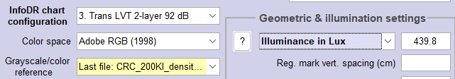
Measure the illuminance E in lux, with the back of the illuminance meter adjacent to the chart, so its sensor facing in the same direction as the chart (the general direction of the light source). Take care not to shade the incident light.
|
| Reflective charts: Luminance measurement (not recommended) |
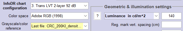
You can also find an equivalent source luminance by measuring a patch with known density, Dpatch. Since density reference files are rarely available for reflective charts (they’re supplied with all transmissive charts, which are less consistent), you need to use a trick. The lightest patch is usually paper white, which has a reflectance of about ρ = 0.92, equivalent to D = -log10(ρ) ≅ 0.04. If the patch is small and shaded by the meter (often an issue with this method), you can use another trick. Use a sheet of white bond paper (or something similar) with a similar appearance to the white patch, placing the meter further from the chart to avoid shading. Since this method is cumbersome and error-prone, it is not recommended. Enter the equivalent source luminance, Lsource = Lpatch ρ into the edit box to the right of the Luminance in cd/m^2 selection in the More settings window, shown below. |
|
Transmissive charts: Recommended for transmissive charts |
There is no illuminance for transmissive charts because they are used in darkened environments, i.e., all illumination comes from behind the chart — from the lightbox. Measure the source (lightbox) luminance, Lsource, either
|
Optionally, the lightbox (source) luminance Lsource in cd/m2 can be calculated by measuring h for a patch whose density Dpatch is specified in the density reference file. You’ll need to point the luminance meter directly at the patch, taking care not to shade it. (This won’t work for very small patches.) The lightbox (source) luminance can be calculated from the measured patch luminance. Lsource = Lpatch / 10(-Dpatch), and read The luminance of each patch is derived from the density file and Lsource .
Photograph the chart
IMPORTANT The chart is designed to be photographed in the central part of the frame.
In most cases, IT SHOULD NOT FILL THE FRAME!
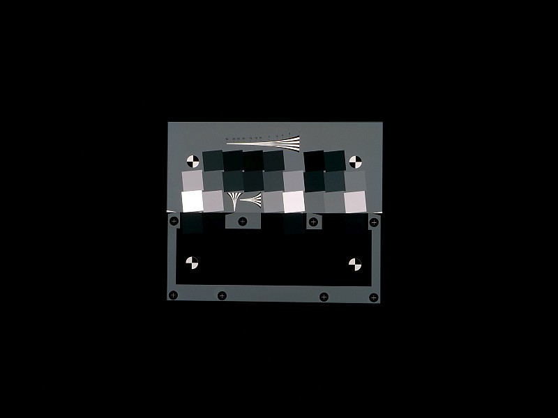
Typical framing, for a 10 Megapixel camera (V1 chart)
If the camera allows exposure adjustment, the chart should be exposed so no more than one or two patches are saturated. The brightest patch should exposed just enough so it’s saturated or close to saturation.
There is one significant difference with traditional SNR-based Dynamic Range measurements:
The chart must be well-focused because edge sharpness is part of the C4 information capacity measurement.
This is one reason the VisNIR chart may be attractive: it can be made 3× larger (linearly; 9× by area) than LVT film charts.
The chart should be framed so the active chart area in in the central portion of the chart. It doesn’t need to be larger than 1000×1200 pixels. Here is an example for a 10 megapixel camera.
Where possible, raw images should be acquired and converted to interchangeable files outside the cameras. JPEG files from cameras often contain bilateral filtering, which sharpens edges and smooths other regions (nonuniform processing), decreasing the accuracy of information metrics.
Low light standards
ISO 19093 is a standard for measuring perceptual aspects of low-light performance — for very different applications from the Imatest InfoDR chart, which focus on information content. Many of the measurements are for the results of intentional signal processing, so processed (i.e., JPEG) images are more appropriate than raw images. For example, measurements include texture and chroma loss in dark regions, both of which are often applied intentionally to optimize perceptual quality, since noise can get ugly in dark regions. Multiple images generally need to be acquired.
The independent variable is scene illuminance L in lux. InfoDR allows a choice of independent variables, including chart patch luminance in candelas/meter2 (cd/m2) and image sensor illuminance in Lux (from ISO 12232). Test chart patches are specified by their densities D, where D = log10(incident/transmitted light) for transmissive charts and D = log10(incident/reflected light) for Lambertian reflective charts. Note that Luminance L in cd/m2 (for the lightbox used with transmissive charts) = Illuminance E / π (for incident light on reflective charts; L = E/π).
| Next: Using InfoDR, Part 2: Analysis |
Appendix: InfoDR chart design and building blocks
The design goal was to have both near-vertical and near-horizontal edges in a compact arrangement so that the camera MTF does not vary by much in the active area of the chart. To that end the two groups of slanted squares with 7 or 8 patches, shown below, contain the basic building blocks.
The lightest patch (reflectance ρ or transmittance τ =1; density D = 0) relative to the base density) is on the lower right of each pattern. The two adjacent patches (to the left and above) have ρ or τ = 1/4, i.e., densities = 0.6. The patch adjacent to previous two patches has ρ or τ = 1/16 = 1/42, i.e., density = 1.2. The next two patches have ρ or τ = 1/64 = 1/43, i.e., density = 1.8. This progression continues as long as needed. Note that the contrast ratio between adjacent patches is always 4:1 (density difference = ΔD = 0.6; Michelson contrast = (ρn–ρn-1)/(ρn+ρn-1) = 0.6).
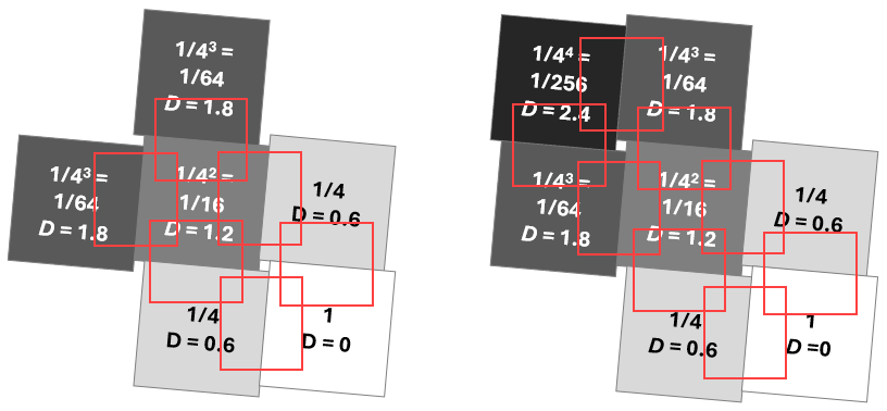 Building blocks of the InfoDR charts. Left: reflective chart; right: transmissive chart (1-layer)
Typical Regions of Interest (ROIs) are shown as red rectangles.
For media that supports higher densities, the chart may be extended diagonally on the upper-left. For example, two patches with transmittance τ = 1/1024 (1/45) or D = 3.0* could be added to the upper-left of the pattern on the right. (*This density cannot be achieved with reflective charts.)
The 4:1 density steps in the building blocks shown above are coarser than ideal for measuring camera performance over a range of illumination. To obtain finer steps, we designed charts with several regions (called quadrants where there are four), where the density of each region is offset from its neighbor by a fined amount that allows small steps throughout the chart’s tonal range. The example below is for the reflective chart, which has four quadrants, each with 6 patches. With this arrangement, the chart has densities from 0 to 2.25 in density steps of ΔD = 0.15 (half an f-stop). Vertical edges are shown as rectangles with cream background; horizontal edges are shown as rectangles with light blue backgrounds. Transmissive charts differ in details: the 2-layer LVT chart has six regions with ΔD = 0.20. The 20layer VisNIR chart has four quadrants with ΔD = 0.30, resulting in an exceptionally high density range at the expense of tonal resolution.
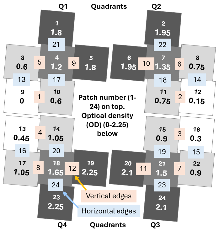 Reflective InfoDR chart: Four quadrants, each offset by D = 0.15 (1/2 f-stop) from its neighbor