
|
Imatest InfoDR (Information-based Dynamic Range) refers to the Imatest module and test charts designed to measure C4 information capacity over a wide range of illumination — especially for low light. This page, Using InfoDR, Part 2 — describes how to analyze the InfoDR charts in Imatest Rescharts and Color/Tone. |
Part 1 – Introduction – C4 Information Capacity – InfoDR chart versions – Lighting – Measuring illumination
Photograph (framing)
Part 2 – Open, Select, & Read – Setup window – Results – Information-related displays
Comparison with traditional DR – More settings – Auto mode – Color/Tone
Appendix: SNRi and Error Probability
|
Using InfoDR, Part 1 — describes the InfoDR charts and how to photograph them. Using InfoDR, Part 2 — describes how to analyze the InfoDR charts in Imatest Rescharts and Color/Tone InfoDR, Part 3 — Results — shows C4 summary results for a number of cameras. Image quality testing based on information metrics (White Paper) A concise guide to camera image quality testing, focusing on metrics derived from information theory, which are more predictive of camera performance than traditional metrics such as sharpness or noise. Image Information Metrics — Introduction and overview of information capacity and related metrics, with links. Using Rescharts — Introduction to Rescharts — an interactive interface for resolution-related charts, all of which can also be run in fixed batch-capable versions. Using Rescharts slanted-edge modules Part 2 — Selecting files – Setup window – ROI selection & analysis – Edge ID files – More settings window – Secondary readout – Settings area – Gamma – Gamma from chart contrast ratio – Auto mode window – Warnings – Clipping – Summary Rescharts Slanted-edge results Part 3 – SFRplus edge results — Multi-ROI summary – Edge and MTF – Chromatic Aberration – Acutance/SQF – Histograms & noise – Image, Geometry, Distortion, FoV – 3D Plots – Lens style MTF plot – Edge roughness – Point Spread Function – Summary – CSV & JSON output Rescharts Slanted-edge results Part 4 – SFRplus other results (tones, color, distortion, etc.) — Tonal response and gamma – Image, Geometry, Distortion, FoV – Radial distortion – Summary and EXIF data – Color analysis – Detailed noise plot – Summary – Links |
|
These instructions are for the InfoDR module, which can run in interactive (Setup) mode or batch-capable Auto mode. Operation is similar to other slanted-edge Rescharts modules, but there are some differences. Most importantly, the InfoDR chart is not designed to fill the field, and the chart type must be specified in the Chart configuration dropdown (or in More settings). We emphasize settings unique to InfoDR. Settings that apply to other Rescharts modules are described in full detail in Using Rescharts slanted-edge modules Part 2. |
We begin with instructions for Rescharts (interactive; Setup) mode, which allows you to enter and modify settings and to explore results. The settings are saved for Auto Mode runs, described below, which allow batches of files to be analyzed.
Open InfoDR, select the chart type, and read the image file
 Normally, Auto ROI detection should be set. It can be found and set in the Dynamic Range … InfoDR setting of ROI Options.
Rescharts Chart configuration
dropdown menu
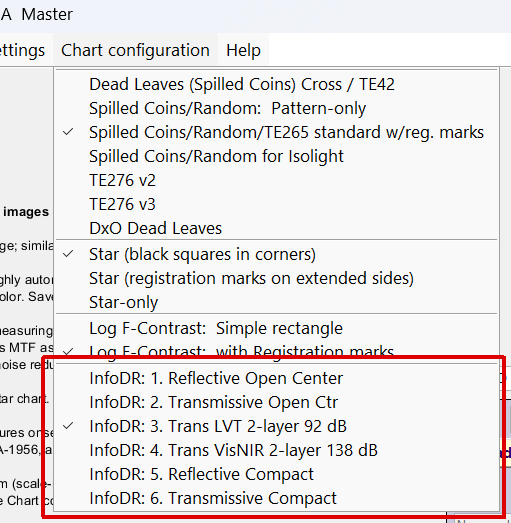
Rescharts analyzes several versions of InfoDR chart, but doesn’t automatically detect them. To see which chart type has been selected, open Rescharts. The specific InfoDR chart type is shown in the Chart configuration dropdown menu, shown on the right. If needed, you can select the correct setting (InfoDR: 3. Trans. LVT 2-layer 92 dB for this example). The setting will be saved. If you know you have the correct setting, you can skip this step. The chart configuration can also be entered in the More settings window.
Select 12. InfoDR in the Chart area on the right to read the image file.
If the correct InfoDR chart type has been saved, open InfoDR to read the image file. Details may differ in the newer and traditional interfaces.
If automatic detection fails, manually set the ROIs by selecting the registration marks and refining the selection.
The InfoDR setup window opens.
InfoDR setup window
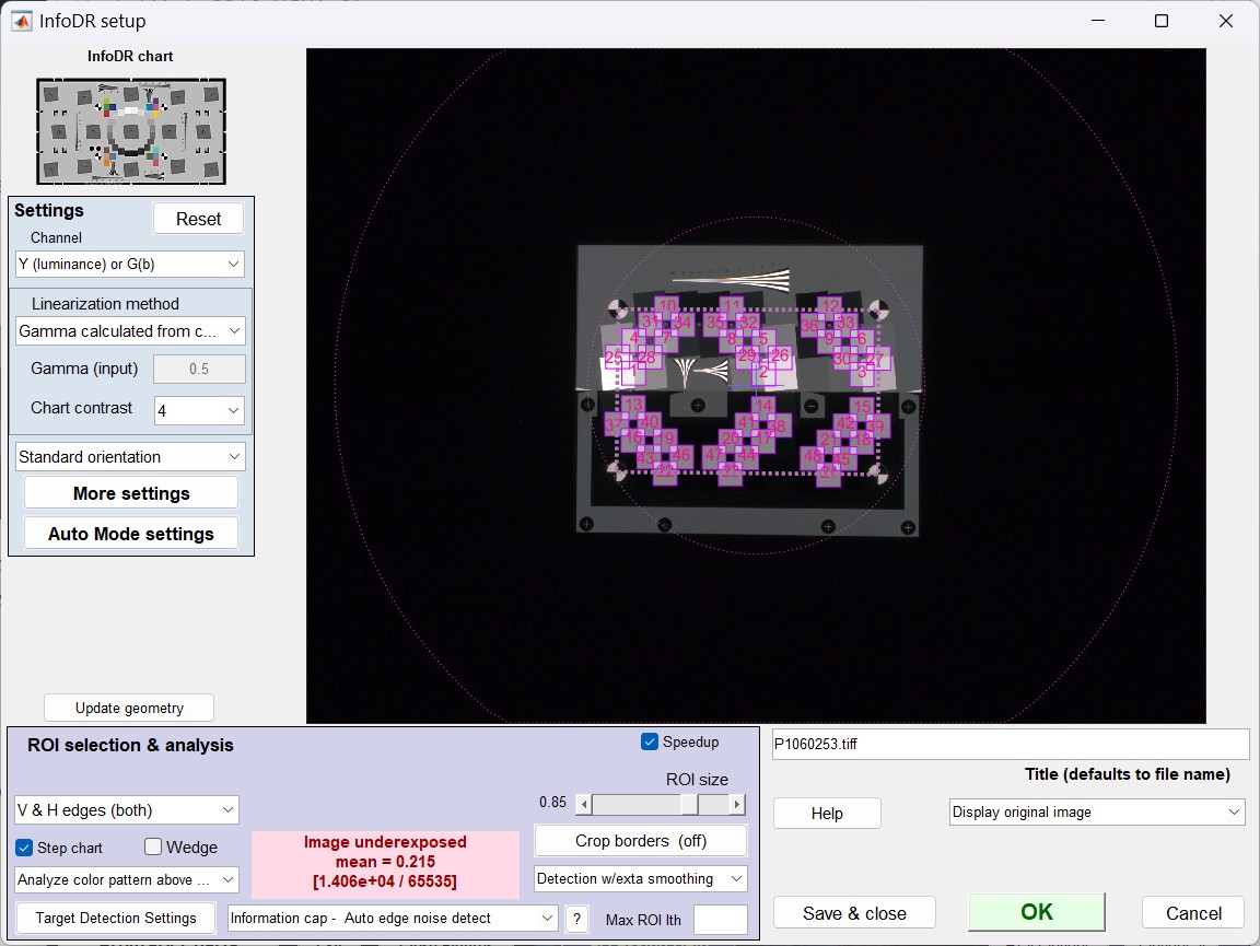 InfoDR setup window
[We will fix some settings that are not quite right. Changes: {Step chart — to be removed) (Wedge — needs more testing)
(Analyze color pattern above — may be removed. Color pattern will be analyzed if a CIELAB (L*a*b*) reference file is used.
Image underexposed will be removed for InfoDR because the active pattern is restricted to the center of the image.
(The area might be shrunk.)]
| Setting | Description & recommendation |
|
Settings area on the left (settings are duplicated in More settings.) |
Used to select the channel for analysis and the linearization method. Typical settings: Y-luminance channel, Gamma selected from chart. See Setup window in Using Rescharts Slanted-edge Modules, Part 2. (The linearization selecting may need to be adjusted to work better with the dark, fogged, and noisy images.) |
| V or H edges | Choose from Vertical, Horizontal, or V&H edges. |
| ROI size | Sets the relative size of the ROI for measuring MTF and noise. 0.8 to 0.9 is typical. |
| Distortion (slider) | Adjust ROI locations if the image is distorted. |
| Crop borders | Rarely used. Only needed if objects in the image interfere with registration mark detection. |
| Detection | Normal or with extra smoothing (best for noisy images– maybe for all images) |
| Info cap | Information capacity settings (should always be on for InfoDR). Lets you select Auto edge detect, Mean noise (best for uniformly-processed — raw-converted images), smoothed peak noise (best for bilateral (nonuniform)-filtered images) |
Click OK to continue with the calculation.
Results
Numerous displays. selected by the dropdown menu just below Display on the right, are available, and many of them have options. The table below is a reference, with links to detailed descriptions. Information displays, highlighted in yellow, are described on this page. All others are on linked pages.
| 1. Edge and SFR (MTF) | Mean edge (top) and SFR (MTF) plot (bottom). Frequently used. |
| 2. Chromatic Aberration | Lateral chromatic Aberration: strongest near edges. Limited value for InfoDR. |
| 3. Acutance / SQF | Visual impression of sharpness. Full description here. |
| 4. Multi-ROI summary | Selected results for multiple ROIs. |
| 5. Tonal Response, Gamma/white Bal | Tonal response and gamma. Learn more about gamma here. |
| 6. Histogram and noise stats | Histogram and edge noise statistics. Rarely used. Speedup must be off. |
| 7. Summary and EXIF data | |
| 8. Image & Geometry | Image, Geometry, Distortion, Field of View. May show ROIs. |
| 9. a*b* Color error | |
| 10. Split colors: Reference/Input | |
| 11. 3D & contour plots | 3D and contour plots of selected variable (there is a large choice). |
| 12. Edge roughness | Edge roughness (not a very good quality indicator; better for blurred images) |
| 13. Noise, SNR, Dyn Rng | Noise, SNR, Dynamic Range. A great many options available. |
| 14. Wedge MTF & aliasing | |
| 15. Wedge moiré | |
| 16. Multi-Wedge summary | |
| 17. Edge & Info Capacity noise | Mean edge (top) and spatially-varying noise (bottom; for information capacity) |
| 18. Info-related: NPS, NEQ, SNRI… | Two plots with a large selection of results (standard and information metrics) for both plots. |
| 19. Info metrics (C_4…) vs. exposure | Information metrics — most importantly C4 — as a function of exposure. KEY RESULT OF InfoDR. |
Information-related displays
Note that More Settings can be called at anytime during interactive analysis, before or after calling displays (which might be affected by the settings).
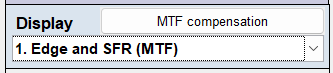 Displays are shown in the Display dropdown menu on the center- right. For InfoDR, the available information-related displays are
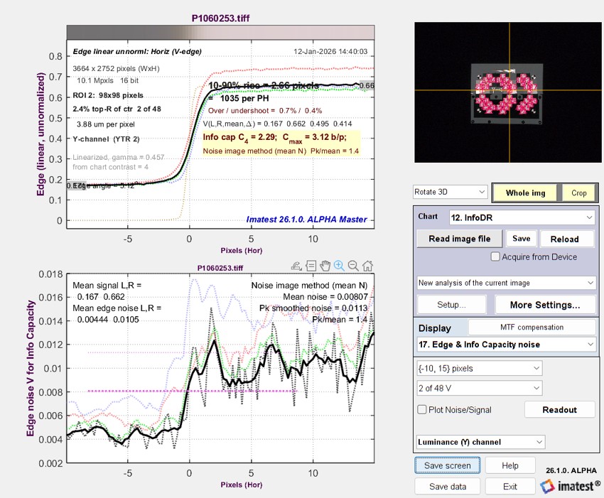
| 1. Edge and SFR (MTF) | Displays Info capacity in Edge plot on top; standard MTF/SFR plot on bottom. |
| 17. Edge & Info Capacity noise | Displays Info capacity in Edge plot on top; spatially-dependent noise on bottom. |
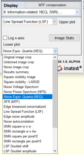
| 18. Info-related: NPS, NEQ, SNRi… | Displays two plots, each with a large selection of results. |
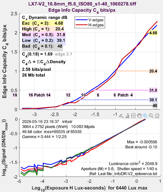
| 19. Info metrics (C_4…) vs exposure | Displays several results (most importantly information capacity C4) as a function of illumination. |
1. Edge and SFR (MTF)
|
 |
|||||||||||||||||||||||||||||||||||||||||||||||||||||||
|
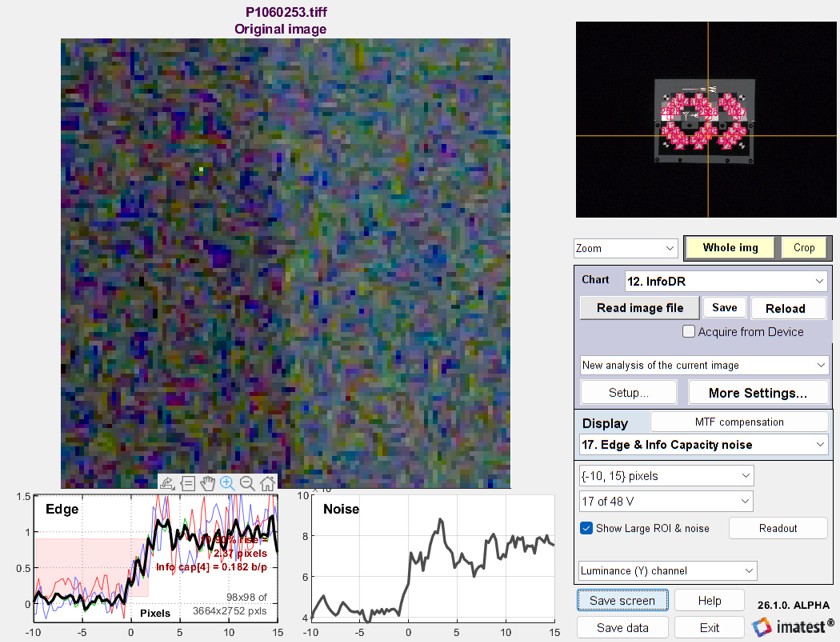
In this plot, Show large ROI and noise has been checked. This displays a large image of the ROI, lightened if it’s dark. This is for a very dark region, where performance is significantly worse than for the light regions.
Enlarged and lightened image of ROI 17, Edge and spatially dependent noise |
 |
|||||||||||||||||||||||||||||||||||||||||||||||||||||||
|
||||||||||||||||||||||||||||||||||||||||||||||||||||||||
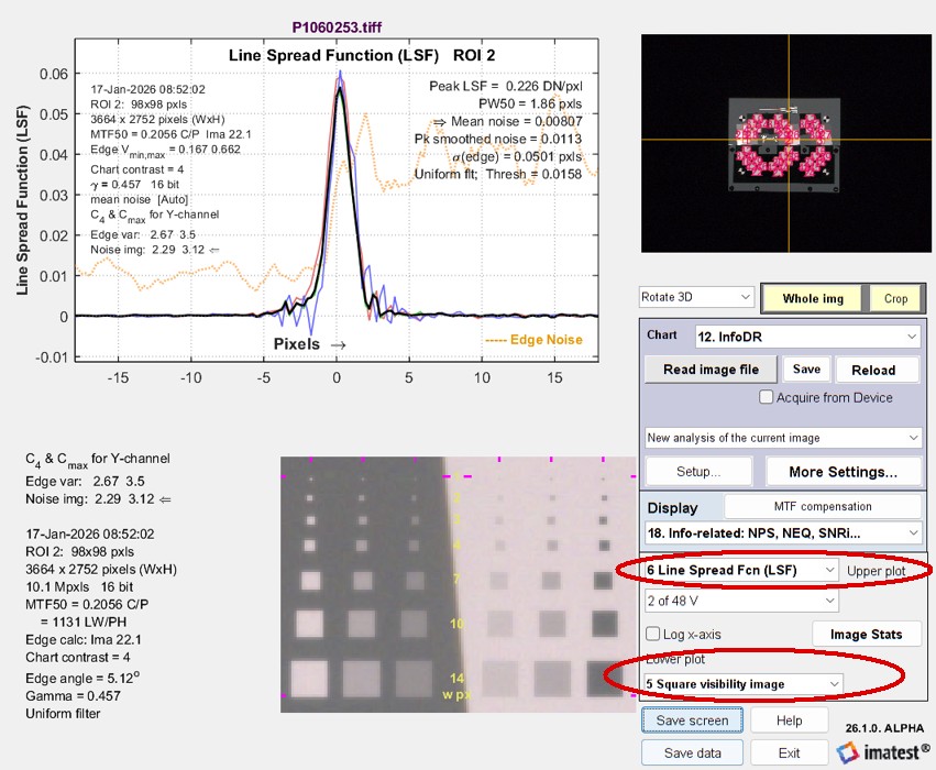 Line Spread function (LSF; upper plot), Line Spread function (LSF; upper plot), Square visibility (lower plot) |
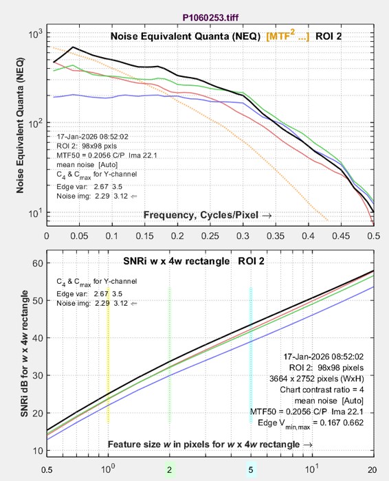 Noise Equivalent Quanta (NEQ; upper plot), Noise Equivalent Quanta (NEQ; upper plot), SNRi (lower plot) |
|||||||||||||||||||||||||||||||||||||||||||||||||||||||
More plot details can be found in Image information metrics from Slanted edges: Instructions — Results 19. Info metrics (C_4…) vs exposureThis plot displays results for multiple regions — from light to dark. It is only available with InfoDR. |
||||||||||||||||||||||||||||||||||||||||||||||||||||||||
|
The upper plot displays the selected variable, from the list below. 1., 3., and 4.
X-axis units can be set to
|
The lower plot displays the density response (log10(signal)). 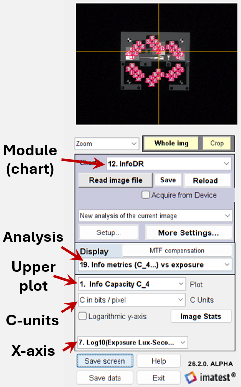 InfoDR control area
Information capacity units (C-units)
|
|||||||||||||||||||||||||||||||||||||||||||||||||||||||
|
The first three x-axis units are relative units based on logarithms: OD (log10), dB (20×log10), and EV (log2). The last three are absolute units, based on illuminance or luminance measurements described in Part 1 of the InfoDR instructions. The last two entries, for Sensor exposure H (the total illumination reaching the sensor in Lux-seconds), are derived from an approximation in ISO 12233:2019, Annex B. |
||||||||||||||||||||||||||||||||||||||||||||||||||||||||
|
SNRi: Ideal Observer SNR for w x 4w pixel rectangles.SNRi is the ideal observer Signal-to-Noise Ration. It indicates object detectability. The rectangle contrast can be adjusted with the Contrast Units dropdown menu (C-units in the above diagram). Higher contrast means higher SNRi and Error Probability.
|
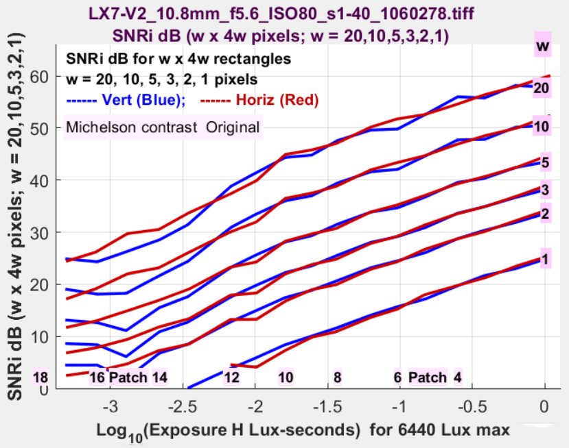 SNRi (dB) for w x 4w rectangles for w = 20, 10, 5, 3, 2, 1 SNRi (dB) for w x 4w rectangles for w = 20, 10, 5, 3, 2, 1 |
||||||||||||||
|
Log10(Error Probability (Bit Error Rate)), derived from SNRi We may modify this curve since a larger number is worse (lower means lower error rates). Rectangle contrast can be adjusted. The challenge in setting specifications (the minimum SNRi or maximum error rate for acceptable performance) is finding the object size and contrast that best correlates with system performance. |
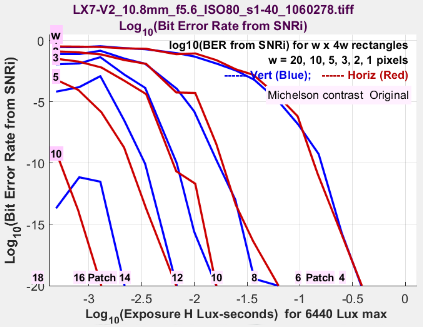 |
Comparison with traditional dynamic range
Information based DR can easily be compared with traditional SNR & slope-based DR by setting Display to 13. Noise, SNR, Dyn Rng and selecting 15. Scene-ref SNR DB & DR. The result is identical to running Color/Tone, described below. Dynamic Range measurements are generally lower than the C4 DR Information-based measurements (above), partly because the damaging effects of stray light are handled better.
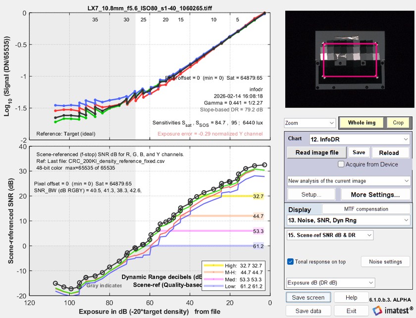 Traditional Dynamic Range measurement from InfoDR chart
More settings window
The More settings window can be called from the InfoDR Setup window at the beginning of an analysis or from the Rescharts window at any time.
Note that some of the settings in More settings are duplicated in the Setup window.
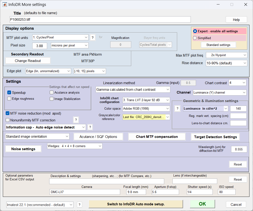 InfoDR More settings window. Many of the settings are shared with other modules and
described in Using Rescharts slanted-edge modules, Part 2 )
| Setting | Description & recommendation |
| Chart contrast | Always 4 for InfoDR |
| InfoDR chart configuration | Select the correct chart configuration from one of the first four (the others are not available): 1. Reflective open ctr, 2. Transmissive open ctr, 3. Trans LVT 2-layer 92 dB (used in the examples on this page), 4. Trans VisNIR 2-layer 138 dB. |
| Color space | Detected automatically (can be changed). Adobe RGB was selected during the LibRaw conversion. |
| Grayscale/color reference | Select the appropriate density reference file. Only available and strongly recommended for 2-layer transmissive charts. |
| Illuminance or Luminance | Make a selection based on the illumination measurement technique (previous page). |
| Information capacity – Auto edge noise detect | Info cap – Auto edge noise detect often works best, especially if processing is unknown, but the other settings (mean for uniformly processed images or smoothed peak noise for bilateral-filtered images) can be used if appropriate. The information capacity calculation must be turned on. |
| Speedup | Checked. Speeds up runs by removing some rarely-needed calculations, like histograms. |
| Linearization method: Gamma calculated from chart contrast | Generally recommended. Other methods are described in Using Rescharts Slanted-Edge Modules, Part 2. |
| Slanted edge calculation (lower-left) | Imatest 22.1 (recommended – defaut). Other settings may not give reliable calculations. |
Click OK to continue with the calculation.
Auto mode
InfoDR Auto runs automatically, without additional input, after the input file (or files for batch mode) are selected. It uses settings saved from Rescharts interactive mode.
The Auto mode settings window can be opened from Rescharts interactive mode from the Settings area on the left side of the Setup window or the wide Switch to InfoDR Auto mode setup button at the bottom of the More settings window.
We don’t recommend any of the Single-region plots. There are simply too many of them to be useful. (Some of them are of interest when running Rescharts interactive mode.) The primary plot of interest is Information metrics (C_4, etc.) vs. exposure. All others are optional, and most are better suited for eSFR ISO, etc.
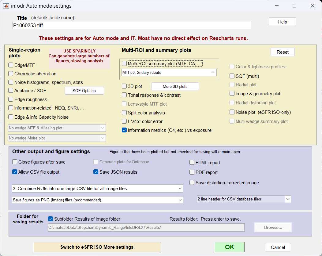 InfoDR Auto mode settings
Color/Tone
|
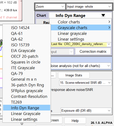
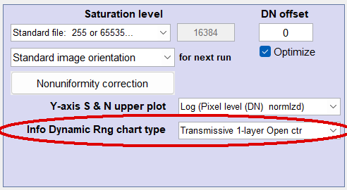
InfoDR charts can also be analyzed from Color/Tone (Interactive or Auto), where they behave like standard dynamic range charts. Color/Tone cannot measure information metrics (C4, etc.). InfoDR is selected from the Color/Tone window as shown near-right. The chart type can be selected from the lower-left corner of Color/Tone settings window, shown far-right and also from the Options II window. |
 |
 |
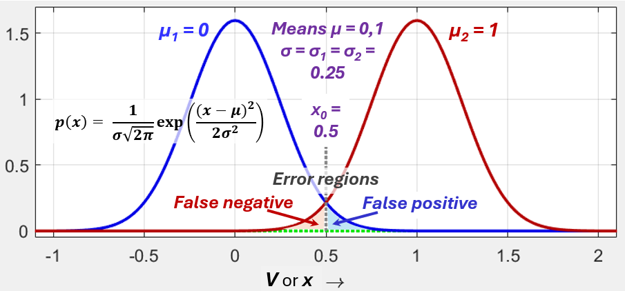
Appendix. SNRi and Error ProbabilityWe use results from detection theory to calculate the total error probability, which is the sum of the probabilities of false positives and false negatives, as illustrated in the Receiver Operating Curve (ROC), below. For the gaussians with means μ1 and μ2 and identical standard deviations σ = σ1= σ2, the minimum error probability occurs when the decision threshold, x0= (μ1 + μ1)/2. Note that the system is symmetrical around x = 0.5. More details on detection theory can be found in Wikipedia and in reference papers.
For the gaussian curves, the probability density function is \(\displaystyle p(x)==\frac{1}{\sigma \sqrt{2 \pi}} \exp \left(-\frac{(x-\mu)^2}{2\ \sigma^2}\right)\) The key assumption is that SNRi can be treated as a standard Signal-to-Noise Ratio (SNR) with signal = Δμ = μ2 – μ1 and noise = σ, illustrated above. \(SNRi\displaystyle = (\mu_2-\mu_1)/\sigma = \Delta \mu/\sigma = 1 / \sigma\) Thanks to the symmetry of the ROC, we can use the left gaussian to calculate the error rate because its mean, μ1 = 0, makes the calculation simpler. The error probability, which we also call Object Detection Error Probability, ODEP (often abbreviated Error Rate of Bit error rate, BER) is \(\displaystyle Pr(x>x_0) = ODEP = Pr(\text{error}) = \int^{\infty}_{x_0} p(x) dx = \int^{\infty}_{x_0} \frac{1}{\sigma \sqrt{2 \pi}} \exp \left(-\frac{(x-\mu)^2}{2 \sigma^2}\right) dx\) For the gaussian curve on the left, the decision threshold is \(x_0=(\mu_1 + \mu_2)/2 = 1/2\). Let \(u^2 = (x-\mu)^2/(2 \sigma^2). \text{ Then } u = (x-\mu)/(\sigma \sqrt{2}) , \ du = dx/(\sigma/\sqrt{2}) , \ dx = \sigma\sqrt{2}\ du\) and \( u_0 = 0.5/(\sigma\sqrt{2}) = 1/(2\sqrt{2}\ \sigma) = SNRi/(2\sqrt{2}) \) . \(\displaystyle Pr(x>x_0) = Pr(\text{error}) = \int^{\infty}_{u_0} \frac{\exp(-u^2)}{\sigma \sqrt{2 \pi}} \sigma \sqrt{2}\ du = \frac{1}{\sqrt{\pi}} \int^{\infty}_{SNRI/(2\sqrt{2})} \exp(-u^2)\ du\) 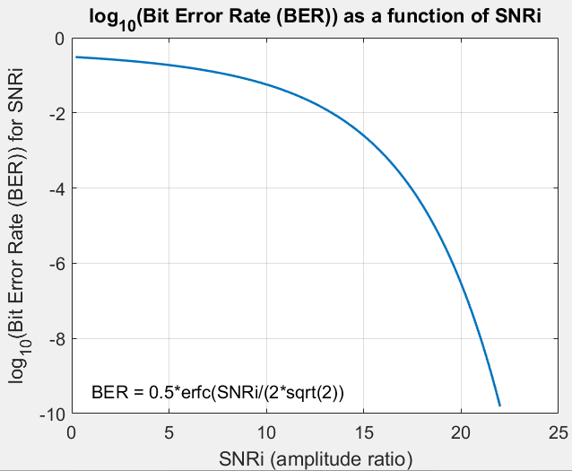 Log10(Error Probability) from SNRi. From the MATLAB documentation for erfc, the MIT class notes, and other sources, \(\displaystyle erfc(z)=\frac{2}{\sqrt{\pi}} \int^{\infty}_z \exp(-u^2)\ du\)
The standard equation for the error rate of BPSK is, \(\displaystyle P_b=Pr(\text{error})=\frac{1}{2}\text{erfc}\left(\sqrt{\frac{E_b}{N_0}}\right)\) There was a discrepancy when we assumed that \(N_0=\sigma^2 ; \sqrt{N_0}=\sigma\), which is explained in the MIT class notes. “We will denote 2σ2 by No. It has already been mentioned that σ2 is a measure of the expected power in the underlying AWGN process. However, the quantity No is also often referred to as the noise power, and we shall use this term for No too.” Based on this statement, it appears that for BPSK, noise power No is measured from the difference between the two gaussians, which is not the same as σ (for a single gaussian). In this case, \(N_0 = \sigma_1^2+\sigma_2^2 = 2\sigma^2 \text{ , and } \sqrt{N_0}=\sigma/2\). Assuming \(\sqrt{E_b} = \Delta\mu/2\) and using \(SNRi = \Delta\mu/\sigma\) , \(\displaystyle P_b=Pr(\text{error}) = \frac{1}{2}\text{erfc}\left(\sqrt{\frac{E_b}{N_0}}\right) = \frac{1}{2}\text{erfc}\left(\frac{\Delta\mu}{2\sqrt{2}\ \sigma}\right) = \frac{1}{2}\text{erfc}\left(\frac{SNRi}{2 \sqrt{2}}\right)\) This resolved the discrepancy we struggled with when we assumed N0 = σ2. |