|
|
The basic premise of this work is that Information capacity is a superior metric It is better than sharpness or noise, which it incorporates, and it can be used |
|
Related pages Image Information Metrics: Information Capacity and more contains key links to documentation, white papers, news, and more on image information metrics. The Electronic Imaging 2024 paper, Image information metrics from slanted edges, contains the best exposition of the image information metrics. The material is also covered in various levels of detail in the white papers listed below.
Information capacity measurements from Slanted edges: Equations and Algorithms (legacy document) contains the most of the equations this page, but we recommend the EI 2024 paper as a reference. The slanted-edge method, which is fast, convenient, and best for measuring the total information capacity, is recommended for most applications, but the Siemens star method (2020) is better for observing the effects of image processing artifacts (demosaicing, data compression, etc.). |
Quick start — Obtaining image information metrics
Background reading: The Electronic Imaging 2024 paper, Image information metrics from slanted edges, is the top choice. The white papers linked from Image Information Metrics: Information Capacity and more are also useful. |
Introduction to the new measurements
This page contains instructions for obtaining image information metrics. These measurements take advantage of newly-discovered properties of slanted edges– Imatest’s most widely used patterns for measuring SFR (MTF). They are unfamiliar to most imaging scientists because most of them were (A) siloed in the medical imaging community, and were traditionally difficult to measure, and/or (B) derived from information theory, which is fundamental to electronic communications, but was difficult to apply to imaging.
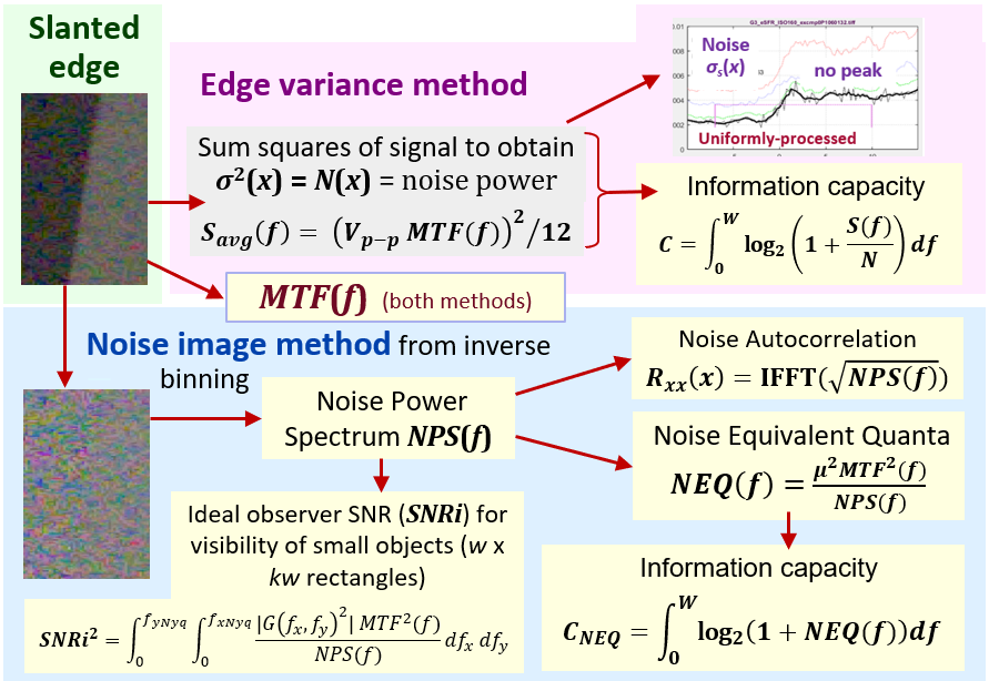
The new metrics are derived from two distinct but complimentary image noise measurements, both of which are made from slanted edges and can be used to calculate information capacity.
- The Edge variance method, conveniently measures spatially-dependent noise.
- The Noise image method measures the noise power (Wiener) spectrum, and uses it to calculate several additional image information metrics (NPS, NEQ, SNRI, Edge SNRi, etc.).
This page introduces the new metrics, shows how to obtain them, then presents a few Key Results.
Detailed algorithms are presented in Information capacity measurements from Slanted edges: Equations and Algorithms.
Calculation summary
A summary of the calculations is presented here for convenience. More details are linked from Image Information Metrics: Information Capacity and more, and especially in the EI 2024 paper, Image information metrics from slanted edges.
A: Edge variance calculation summary
Sum the scan lines to obtain the mean edge.
Starting with images of slanted edges, (Original ROI, below), typically made from a 4:1 contrast chart (though chart contrasts between 2:1 and 10:1 are acceptable), the standard slanted-edge algorithm
- finds the center of each scan line (taken in a horizontal or vertical direction approximately normal to the edge),
- fits the centers to a polynomial curve, then,
- depending on the location of the polynomial at the scan line, it adds the contents of the scan line to one of four bins.
- The mean values of each bin are then interleaved to form a 4× oversampled edge, μs(x), which has lower noise than the individual scan lines.
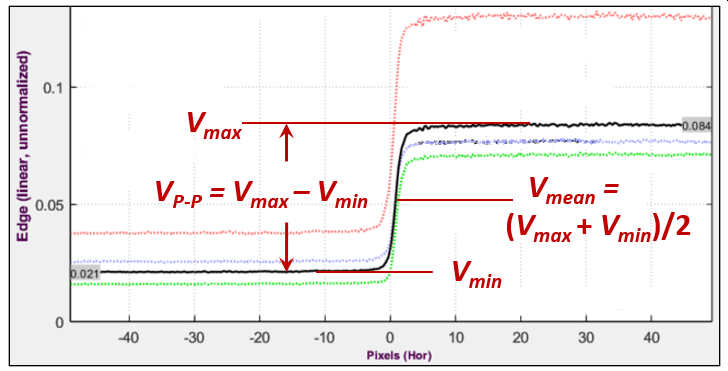
Statistics from slanted-edge Voltage V(x)
Next, add the squares of each scan line to the appropriate bin to calculate the variance of the edge signal, σs2(x), which is equivalent to its noise power, N(x).
- The Shannon-Hartley equation for information capacity is \(C=\int^W_0 \log_2\left(1+S(f)/N(f)\right)\), where S(f) and N(f) are signal and noise powers, respectively, and W = 0.5 C/P is the bandwidth. The noise power spectrum (N(f)) is assumed to be approximately flat for this method.
- The signal is assumed to be uniformly distributed over VP-P, which results in the maximum information capacity. The mean signal power is \(S_{avg}(f)=\left(V_{P-P}\ MTF(f)\right)^2/12\).
- For minimally or uniformly processed images, the mean noise power is used for N(f).
- For bilateral-filtered images (sharpened near edges; smoothed elsewhere; found in most JPEGs from cameras), the smoothed peak noise power is used for N(f).
The key results are,
C4 is the Shannon information capacity measured directly from 4:1 contrast ratio slanted-edges. C4 is a special case of Cn, for a n:1 contrast ratio (with ISO standard 4:1 strongly recommended) Cn is sensitive to chart contrast ratio and exposure, making it useful for measuring performance as a function of exposure, but C4 is not a direct measurement of a camera’s maximum information capacity.
Cmax is a much more stable measurement of the maximum information capacity for the camera. It is derived fromC4. It is also insensitive to exposure, at least for linear sensors, where noise is a known function of signal.
B. Noise image calculation summary Full details here
Subtract a low-noise unbinned / reverse-projected ROI image to obtain a noise image.
This method involves inverting the ISO 12233 binning procedure. Noting that the 4× oversampled edge was created by interleaving the contents of 4 bins, we apply an inverse of the binning algorithm to set the contents of each scan line to its corresponding bin (Inverse binned… ROI, below). Since the inverse-binned image is nearly noiseless, a noise image can be created by subtracting the inverse-binned image from the original image. This image is scaled using Parseval’s theorem, which states that the integral of the noise power spectrum equals the integral of the spatial power. \(\int N(f)df = \int N(x)dx\) for noise powers N(f) and N(x). The noise image is displayed by adjusting the mean (zero) value to be middle gray, is illustrated as the Noise image, below.
| Measurement | Description |
| Noise Power Spectrum, NPS(f) | NPS(f) is implicitly assumed to be constant (white noise) in the Edge variance method. The noise apliitude (voltage) spectrum in \(\sqrt(NPS(f)\). |
| Noise autocorrelation | The inverse Fourier transform of the Noise Voltage Spectrum. Related to sensor electrical crosstalk. Experimental. |
| Noise Equivalent Quanta, NEQ(f) and NEQinfo(f) |
measures of frequency-dependent signal-to-noise ratio (SNR). \(NEQ(f) = \mu^2\ MTF^2(f) / NPS(f)\text{, where }\mu = V_{mean}\) has been used for quantifying medical image quality, but are much less familiar in general imaging. NEQ(f) is equivalent to the number of quanta detected by the sensor when photon shot noise is dominant. It is appropriate for calculating Digital Quantum Efficiency (DQE), when the density of quanta reaching the image sensor is known. NEQinfo(f) is derived from \(\mu = V_{P-P} / \sqrt{12}\), making it well-suited for calculating information capacity CNEQ. |
| Information capacities C4-NEQ and Cmax-NEQ |
correspond to C4 and Cmax from the Edge variance method, but are derived from NEQinfo(f). They are close, but not identical. |
| Ideal observer Signal-to-Noise Ratio, SNRi |
From Skorka and Kane [9], “The Ideal Observer is a Bayesian decision maker that maximizes the statistical precision of a hypothesis test with two possible outcomes.” SNRi is a metric of the detectability of objects (squares or rectangles). |
| Edge SNRi | Edge SNRi is a metric of the detectability of edges (obtained from the gradient of the object). |
Simulating the effects of image processing
The effects of sharpening and lowpass filtering can be simulated to predict their effects on object and edge detection performance. This can be used to answer a number of important questions, such as,
- How much do the key object and edge detection metrics (SNRi and Edge SNRi) change as filter settings (lowpass filter cutoff frequency and sharpening amount and radius) are adjusted? This is important because real-world systems have to work with a variety of objects and situations, and therefore successful ISP design involves tradeoffs.
- Does strong oversharpening, which we frequently see in customer images (visible as in “halos” near edges and strong peaks in the MTF response), degrade the key object and edge detection metrics?
See Image Processing for Image Information Metrics for the full instructions on how to apply image processing.
Acquire the image
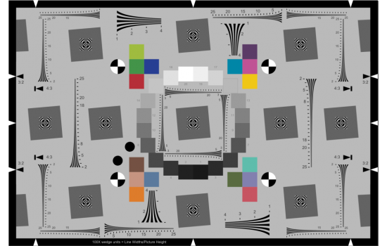
The eSFR ISO chart. Automatically detected ROIs, combining MTF, color, tone, and noise measurements
Acquire a well-exposed image of any slanted-edge test chart (SFRplus, eSFR ISO, Checkerboard, SFRreg, or SFR) in even, glare-free light. Chart edge contrast ratio should be 4:1 (the ISO 12233 standard) where possible. The limits are 2:1 to 10:1. For the most part, acquiring the image is identical to standard MTF measurements.
If you are not sure which slanted-edge chart is best for your needs, there is a comparison table in the main documentation page.
Exposure consistency is important when comparing cameras because exposure affects the information capacity measurement. (Exposure has only a second-order effect on MTF measurements.) If possible, the mean pixel level of a perfectly exposed slanted-edge region should be in the range of 0.20 to 0.26, but there is plenty of latitude as long is the image isn’t saturating.
On the other hand, measuring C4 as a function of exposure may be of interest where low-light performance is a concern.
For best results the slanted edge regions of interest (ROIs) should be 100 pixels or more along the edge. Fewer pixels will give less consistent results.

ROI showing JPEG artifacts. For best results, the edge should be centered in the ROI.
Tips for acquiring images
Uniformity — The chart should be illuminated as uniformly as possible. Simple (first-order) nonuniformity can be corrected,. Charts that are not mounted flat may have nonuniformities (kinks) that cannot be corrected, resulting in serious degradation of information capacity.
JPEG artifacts — with low-quality JPEGs can be really ugly and seriously degrade measurements. The example on the right, enlarged 4×, illustrates both JPEG artifacts and kinks. This image had significant noise reduction at a distance from the edge, and low quality compression may have been applied in the website used to transmit the image. If an image needs to be saved as a JPEG to keep it small enough for an email attachment, make the JPEG very high quality.
Run the MTF calculation module
Run the appropriate slanted-edge module, either in
- Rescharts (interactive; recommended for making settings and testing them) — SFRplus Setup, eSFR ISO Setup, SFRreg Setup, or Checkerboard Setup, or SFR, or
- an appropriate fixed, batch-capable module (SFRplus Auto, eSFR ISO Auto, Checkerboard Auto, SFRreg Auto, or SFR).
Recommended settings
Before calculating the image information metrics, a few settings are recommended.
Information capacity calculation
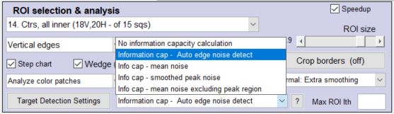
In the Settings window, select the appropriate setting in the Information capacity display dropdown menu. It may be somewhat inconspicuous. Calculating information capacity slows down operations slightly. Two examples are shown below. This setting is also in the SFR Setup and Rescharts SFR Setup windows.
 information capacity noise calculation setting, from a crop of information capacity noise calculation setting, from a crop ofthe Rescharts Settings window for auto-detect slanted-edge modules |
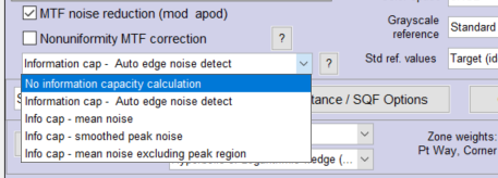 Information capacity noise calculation setting, Information capacity noise calculation setting,from left side of Rescharts More settings window |
The full windows and complete instructions are in SFRplus, eSFR ISO, Checkerboard, SFRreg, or SFR.
The reason for the different noise calculations is
- uniformly or minimally-processed images, often converted in the computer from raw images, pictured here, have relatively uniform noise, which is somewhat signal-dependent where photon shot noise is dominant. There is no noise peak near the transition. Hence the mean edge noise in the ROI is most appropriate.
- bilateral-filtered images, including most JPEGs from consumer cameras, pictured here, are sharpened near the transition and noise-reduced (lowpass-filtered) elsewhere. Hence the average noise would be too low to represent system performance. Hence the (smoothed) peak noise is most appropriate.
- The presence or absence of a peak can be used to detect bilateral filtering (for setting 2: Auto edge noise detection), but it’s not entirely accurate since blurry images may exhibit little peak.
If an information capacity calculation is selected (2-5, below), both Edge variance and Noise image calculations are performed. These settings affect the Edge/MTF display, which has limited space. Results from both methods are displayed in the Noise Spectrum, NEQ, SNRi plot when Results summary is selected for the lower plot.
| # | Setting | Description | Best for |
| 1. | No information capacity calculation | slightly faster than calculating information capacity. About the only time it’s appropriate is for high-speed realtime image acquisition. | Fastest, but not by much since info cap calculations are turned off during reloads. |
| 2. | Calculate info cap: Auto edge noise detection | Selects the noise calculation method depending on the detection (presence or absence) of a noise peak. Recommended for most images. Selections 3 or 4 are OK if the image processing is known and consistent (either minimally/uniformly processed or bilateral-filtered). | for unknown image processing: “black box” |
| 3. | Info cap using mean edge noise (for uniformly/minimally processed images) | for images converted from raw with minimal or uniform processing (no bilateral filtering). | for uniformly / minimally processed images |
| 4. | Info cap using smoothed peak noise (for bilateral-filtered images) | for bilateral-filtered images, which includes most JPEG images from consumer cameras. It works for uniformly-processed images, but gives less stable results than Method (1). | for bilateral-filtered images (most consumer camera JPEGs) |
| 5. | Info cap using mean edge noise excluding peak region | Added when a dust speck caused a spurious peak to appear in a uniformly sharpened image. Mostly fixed now. Normally the same as 3. |
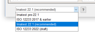
Binning — In the lower-left of the More settings window, choose one of the Imatest edge calculations, preferably Imatest 22.1 (recommended). At this writing it produces the most reliable results.
Linearization method — Several are available. If the chart contrast is know (pretty much required for information capacity measurements), enter the chart contrast (4 recommended) and select Gamma calculated from chart contrast. This setting doesn’t make a big difference, but this choice is quite robust when cameras with different image processing are to be tested.
Miscellaneous settings — Check Speedup (avoids unneeded calculations), MTF noise reduction (mod apod) (a minor cleanup of noisy results). If there is visible illumination nonuniformity, check Nonuniformity MTF correction.
Noise settings (which may not affect information metrics) can be made from a button in the Rescharts More settings window.
When settings are complete, press OK to analyze the image. Any display can be selected, but only a few (shown below) are for information metrics. The same results can be obtained from running fixed modules.
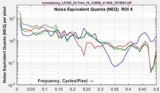
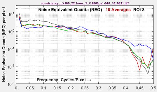
Smoothing rough results with signal averaging
Sometimes results such as MTF or NEQ (or any results) can be rough for noisy images. This happens because slanted-edge Regions of Interest (ROIs) are often smaller than optimum. A reliable fix for this issue is signal averaging: acquiring multiple identical images, then averaging them for analysis. Averaging Navg signals improves the Signal-to-Noise Ratio (SNR) by the square root of Navg (an improvement of 3 dB for every doubling of Navg).
For information capacity/SNRi/NEQ calculations, Noise power is multiplied by the number of averages, Navg. This does not cause a systematic change in the results — it just makes them more consistent.
Here are examples of the improvements from signal averaging.
| Noisy image (ISO 12800) | Noisy image, navg = 10 averages |
 |
 |
 |
 |
Benefits of signal averaging
|
Signal averaging works with almost any Imatest analysis module. |
Instructions for signal averaging
- Read a batch of N images (using the usual methods of selecting multiple files). The settings window shown below appears. A warning will appear if the files are not equal in size.
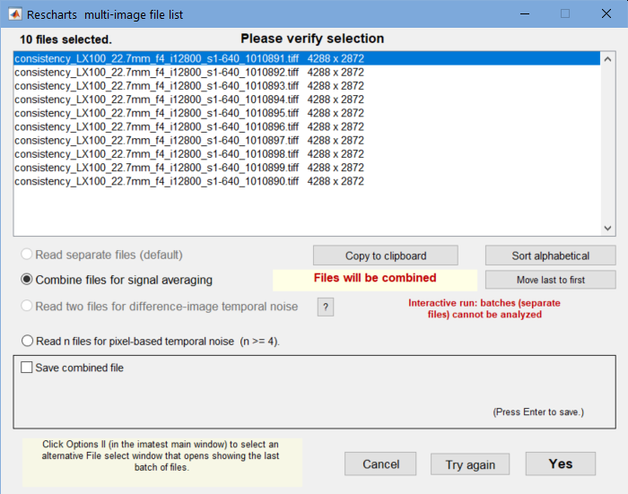
- Select Combine files for signal averaging. The Save combined file checkbox is optional.
- if settings are correct, press Yes. The analysis will proceed.
Results: Edge variance method & older
Edge/MTF plot
Information capacity (for the individual edge) has been added to the upper (Edge) plot. Nothing else has changed.
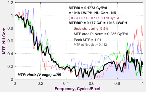
The image below is from a raw-converted eSFR ISO chart image from a high quality compact camera.
 Edge/MTF Results from eSFR ISO image converted from raw with minimal processing
Both information capacity C4 (for 4:1 contrast charts; very sensitive to exposure) and Cmax (maximum information capacity; relatively insensitive to exposure) are displayed.
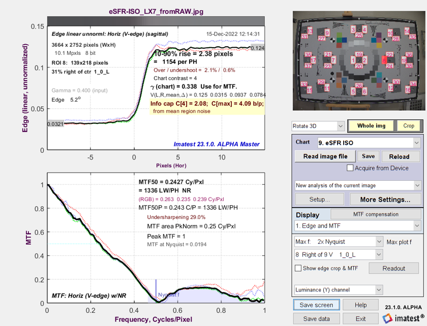
Edge & Info Capacity Noise
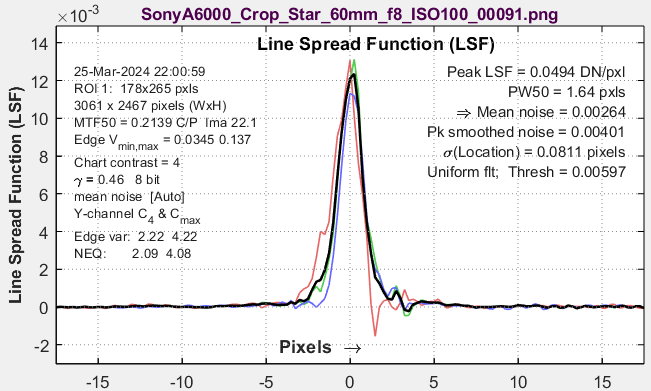
This is a variant of the Edge and MTF plot. The top plot is similar (though the Line Spread Function — the derivative of the edge — is of special interest for this plot).
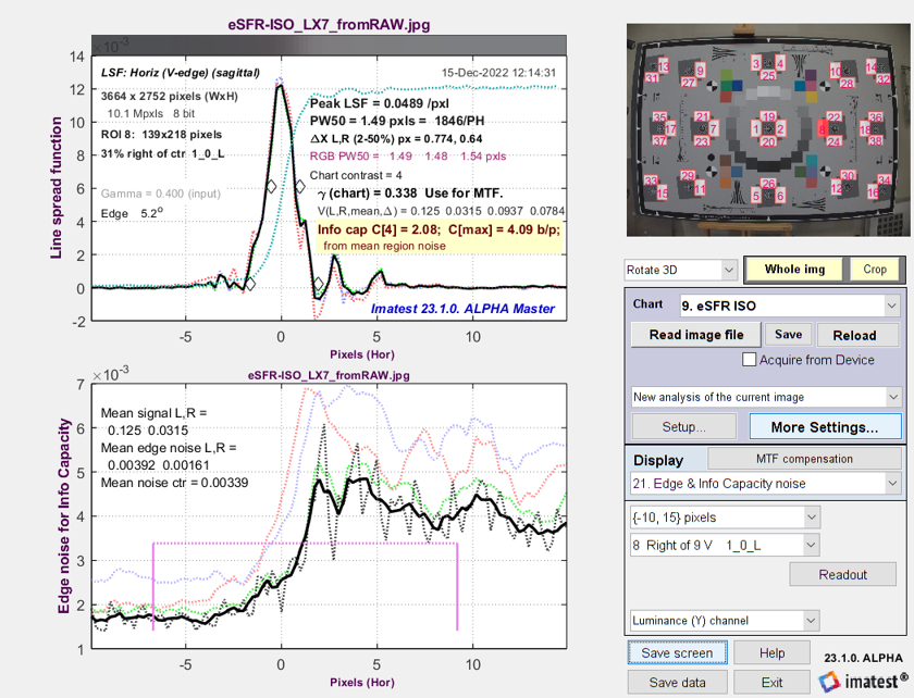 Line Spread Function (LSF) and signal-dependent noise σ from
eSFR ISO image converted from raw with minimal processing
The solid line is the noise smoothed by a rectangular kernel with width = 5 (4× oversampled) pixels (1.25 original pixels). Note that the noise is very rough and that there is no distinct peak near the edge transition. From observing regions of the chart, the bumps on the noise curve appear to be random and not repeatable.
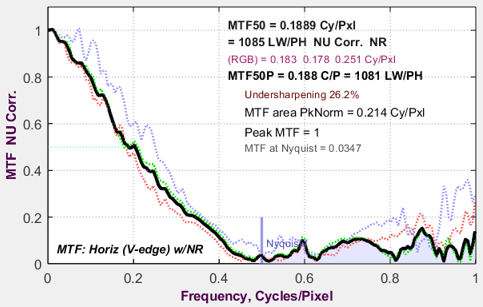
Now it gets interesting. The image used for the above plots is derived from a raw image with minimal processing (straight gamma curve; no sharpening or noise reduction — and definitely NO bilateral filtering). Here are results for the in-camera JPEG from the same acquisition. Note the large noise peak near the edge. We use Method (1) to calculate noise for the Shannon-Hartley equation, which takes the average over a fairly wide region near the edge.
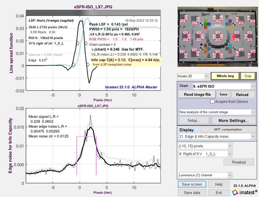 Line Spread Function (LSF) and signal-dependent noise σ from
eSFR ISO image captured as a JPEG (with strong sharpening and bilateral filtering)
Method (2): Calculate noise for info cap using the maximum value of the smoothed edge noise. This method is recommended for bilateral-filtered JPEGs because it uses a relatively narrow region near the noise peak for measuring noise. Information capacity C4 = 3.11 b/p is only slightly higher than for the TIFF: 3.0 b/p. If Method (1) (averaging over a large area, which doesn’t emphasize the peak) is chosen, C4 = 3.84 b/p: significantly larger than the raw measurement, and clearly not accurate.
3D plot and total information capacity
C4 and Cmax have been added to the available 3D plots.
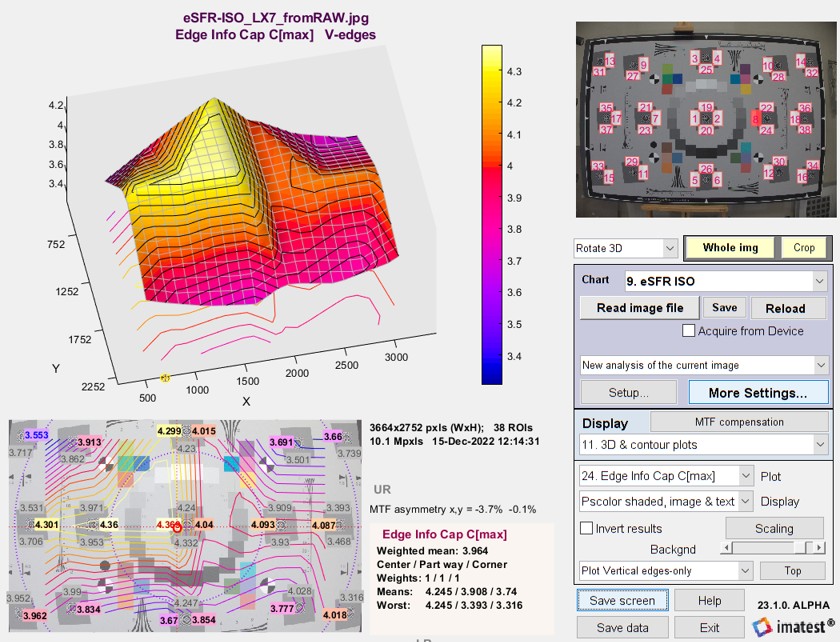 3D plot of Edge Information capacity C4
The total information capacity Ctotal (referenced to the signal level: in this case 4:1) is calculated by multiplying the weighted mean (with all weights are set to 1 for the two information capacity plots) in bits per pixel by the total number of megapixels. It is displayed next to the mean information capacity (in bits per pixel).
In the above image, Ctotal = 2.847 bits/pixel × 16 megapixels = 45.44 megabits. The display shows Edge Info Cap Cmax Mean: 2.847; total Mb: 45.44.
Information-related: NEQ, SNRi, … display
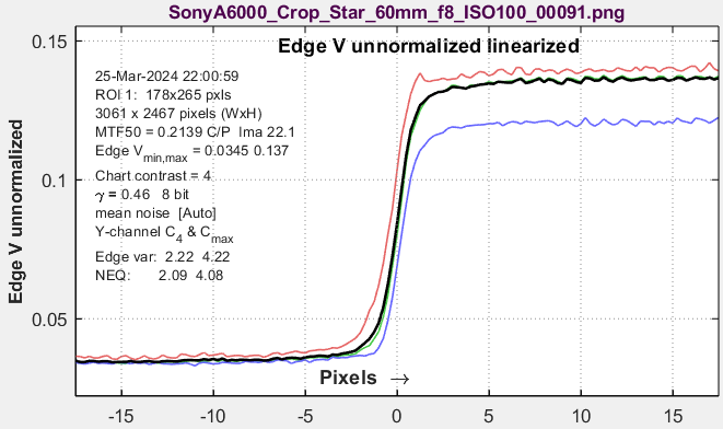
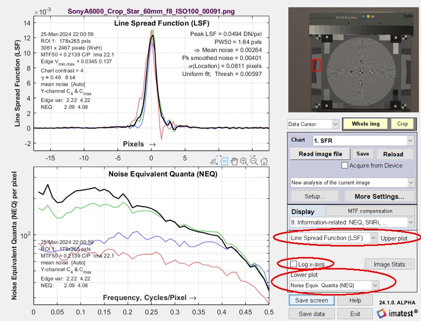 Image information metrics (NPS, NEQ, SNRi, Edge SNRi, and more) as well as several traditional metrics (MTF, LSF, …) are displayed in the Information-related: NEQ, SNRi, … display.
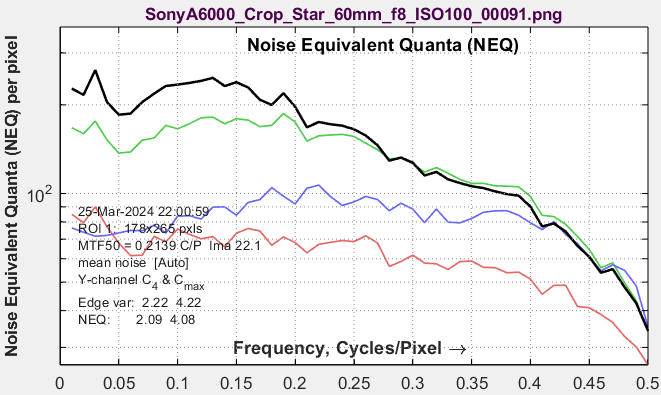
A 24 megapixel Micro Four-Thirds camera with a high quality 60mm prime (macro) lens set to f/8 and ISO 100 was used to obtain these results. All color channels are displayed.
A key feature of the Information-related… plot is that it displays two results: one at the top and one at the bottom, making it easy to compare and correlate different results. This feature was used extensively during the development of the new metrics.
Rescharts display of Line Spread function (LSF; upper plot) and
Noise Equivalent Quanta (NEQ; lower plot)
The Log x-axis checkbox between the two dropdown menus (shown inside a red oval on the right) lets you select a linear or logarithmic x-axis for frequency plots.
|
A large selection of results is available in the Information-related… dropdown menus for the upper and lower plots, shown inside the red ovals in the Rescharts Display area, above right. The Information-related… dropdown menu is something of a monster. It contains more entries than ideal (you have to scroll to see them all). It might change in a future release. |
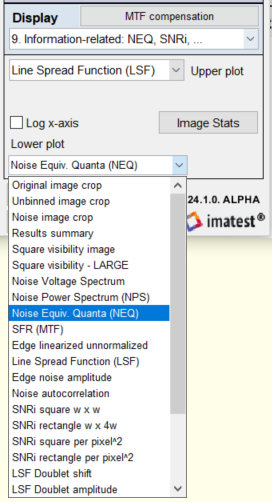 |
| Upper and Lower plots | Notation is from the EI2024 paper. |
| Noise Voltage Spectrum | NPS(f) Also called the Wiener spectrum. An important intermediate result used to calculate the Kernel, \(K(f) = SFR^2(f)/NPS(f)\) and other key metrics. |
| Noise Power Spectrum (NPS) | \(N_V(f) = \sqrt{NPS(f)}\) |
| Noise Equiv. Quanta (NEQ) | A frequency-dependent SNR power that represents the number of quanta incident on a pixel for photon-dominated signals. \(NEQ(f) = \mu^2\ K(f)\) |
| SFR (MTF) | Spatial Frequency Response (synonymous with Modulation Transfer Function). Key measure of sharpness. |
| Edge linearized unnormalized | μS(x) The average edge (the output of the ISO binning algorithm) |
| Line Spread Function (LSF) | \(LSF(x) = d \mu_S(s)(x) / dx\) The derivative of the edge |
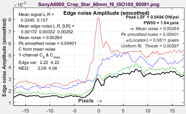
| Edge noise amplitude | \(\sigma_S(x) = \sqrt{N(x)}\) |
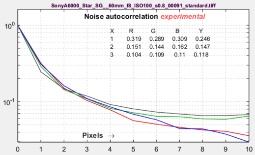
| Noise autocorrelation | IFFT(NEQ(f)) An experimental measurement related to sensor crosstalk. |
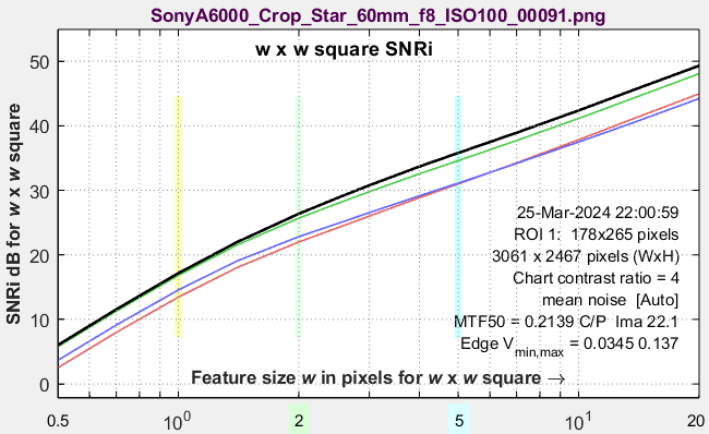
| SNRi square w x w | Ideal Observer SNR for square objects (with w × w pixel sides). |
| SNRi rectangle w x 4w | Ideal Observer SNR for rectangular objects (with w × 4w pixel sides). |
| SNRi square per pixel^2 | SNRi per pixel2 for a w×w square. Levels off; doesn’t increase indefinitely. |
| SNRi rectangle per pixel^2 | SNRi per pixel2 for a w×4w rectangle. Levels off; doesn’t increase indefinitely. |
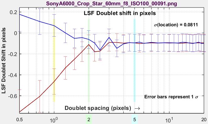
| LSF Doublet shift | Line Spread Function doublet shift as a function of spacing |
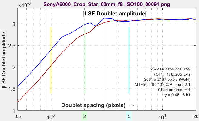
| LSF Doublet amplitude | Line Spread Function amplitude as a function of spacing |
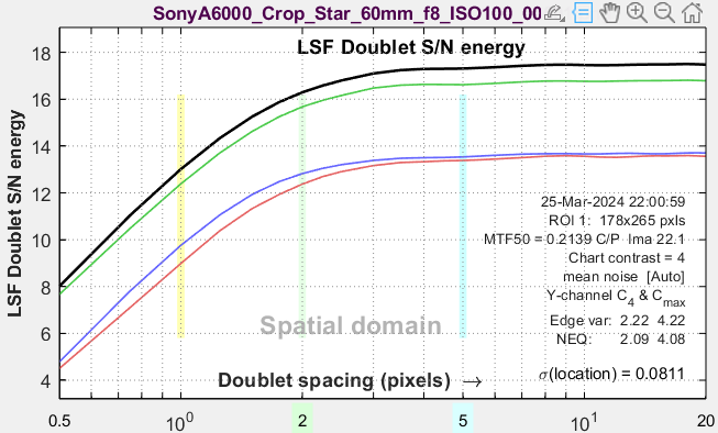
| LSF doublet S/N energy | Line Spread Function energy as a function of spacing |
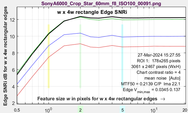
| Edge SNRi square w x w | Edge SNRi for a for a w×w square. |
| Edge SNRi rectangle w x 4w | Edge SNRi for a for a w×4w rectangle. |
| Edge SNRi 1D doublet | Edge SNRi for a for a long 1D object. |
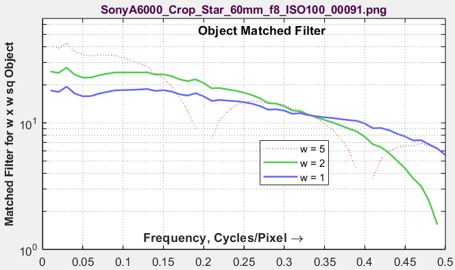
| Object matched filter | Fmatched-object(f) Response of matched filter that optimizes SNRi |
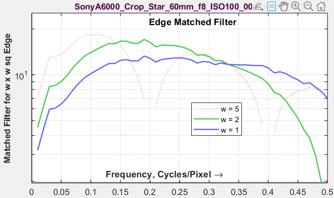
| Edge matched filter | Fmatched-edge(f) = f × Fmatched-object(f) Response of matched filter that optimizes Edge SNRi |
| Lower plot-only | |
| Original image crop | The original (input) ROI |
| Unbinned image crop | Reverse-projected; low noise |
| Noise image crop | Original image – Noise image, lightened and contrast-boosted for display. |
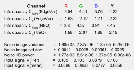
| Results summary | Text showing C4 and Cmax from the Edge variance and Noise image methods, as well as other results, some of which are experimental and may change. |
| Object visibility image | A synthetic image showing the visibility of squares of various sizes (1×1 to 14×14 pixels) and Michelson contrasts (0.6 for 4:1 chart contrast, 0.3, and 015). The LARGE version covers both the lower and upper display areas. |
| Object visibility – LARGE | |
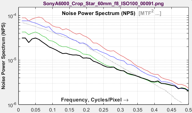
Noise Power or Voltage Spectrum (NPS)The Noise Power (Wiener) and Voltage Spectrum plots have the same shape: only the y-axis labels are different. NPS is an intermediate calculation, used to calculate many of the image information metrics. The 1D Noise Power or Voltage spectrum is derived from a 2D Fourier transform (FFT) of the noise image. The initial 2D FFT has zero frequency at the image center. The image is divided into several annular regions, and the average noise power is found for each region. |
 |
Noise Equivalent Quanta (NEQ)The standard NEQ used in the plot is based on the mean signal voltage, Vmean, shown above. A different voltage, VP-P /sqrt(12), is used to calculate NEQ-based information capacity, CNEQ. The NEQ plot is rough because of the relatively small size of the slanted-edge ROIs (Regions of interest). |
 |
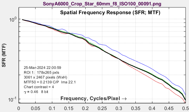
Spatial Frequency Response (SFR / MTF)Note that the y-axis is logarithmic. The x-axis can be either linear (shown) or logarithmic. This plot looks a little different from MTF in the standard Edge/MTF plot because the y-axis is logarithmic. |
 |
Edge linearized unnormalized, V(x)Also in the standard Edge/MTF plot. Useful for observing overshoots from sharpening. Used to calculate Signal Power, S, for the Shannon-Hartley equation in the Edge Variance calculation. |
 |
Line Spread Function, LSF(x) = dV(x)/dxAlso in the Edge & Info Capacity noise plot, shown above. MTF(f) = |FFT(LSF(x))|, normalized to 1 at zero frequency. Bilateral-filtered images have a noise peak in the vicinity of the edge, where LSF has its maximum value. |
 |
Edge noise amplitudeSmoothed with a 1.25 pixel smoothing kernel. Also in the Edge & Info Capacity Noise plot, shown above for minimally processed and bilateral-filtered images from the same image capture. A peak in this plot indicates a bilateral-filtered image (common in JPEGs from consumer cameras). |
 |
Ideal observer Signal-to-Noise Ratio (SNRi) for a square or rectangleSNRi is an indicator of the detectability of small objects. It can be displayed for a square of sides w and rectangles of sizes w × 4w for w = the length of the smaller side in pixels. SNRi is discussed in detail in papers by Paul Kane [8] and Orit Skorka and Paul Kane [9]. A problem with the SNRi display is that it can become very large as sides w increase. This makes it hard to interpret visually. Equations/algorithms EI 2024 paper, Equations (17-20), Figure 20 |
 |
SNRi [square or rectangle] per pixel2Easier to interpret visually than plain SNRi, though it doesn’t quite flatten out. |
|
Edge SNRiSimilar to SNRi, but based on the edges rather than the object bulk properties. Shown for w×w squares, w×4w rectangles, or 1D doublet objects. Does not increase indefinitely as object size increases. |
 |
Object Matched FilterShows the transfer function (frequency response) of a filter that has the best Edge SNRi for objects with widths 5, 2, and 1 pixel. Equal to the transfer for the object MF × frequency. Can be approximated with real filters. We will need to determine best practices for designing a filter that trades off object and edge performance. |
 |
Edge Matched FilterShows the transfer function (frequency response) of a filter that has the best Edge SNRi for edges with widths 5, 2, and 1 pixel. Can be approximated with real filters. We will need to determine best practices for designing a filter that trades off object and edge performance. EI 2024 paper, Equation (27), Figure 29 |
 |
|
Shows doublet shift in pixels as a function of spacing in pixels, displayed logarithmically. Not a major result. |
 |
|
Shows doubled amplitude as a function of spacing in pixels, displayed logarithmically. Not a major result. |
 |
|
LSF Doublet S/N energy (spatial domain) Shows doubled energy (∫ amplitude2) as a function of spacing in pixels, displayed logarithmically. Comparable to Edge SNRi for the 1D doublet. Not a major result. |
 |
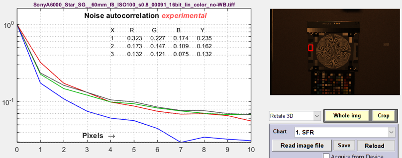
Noise autocorrelation (related to sensor electrical crosstalk)
|
 |
|
The image on the right was not White-Balanced. The red channel has a larger autocorrelation distance than the other channels, as we would expect. Click on the image to enlarge it. A similar autocorrelation plot can also be obtained from a flat field image in the Image Statics module. Illumination nonuniformity was corrected to decrease the autocorrelation at large distances. |
 |
Lower plots-only Displayed in the lower-left of the Rescharts window
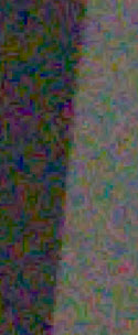
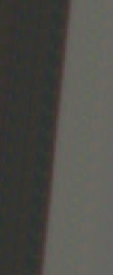
Image ROI crops (original, unbinned, noise)We illustrate crops of the ROI here for a noisy image (ISO 12800), where the difference between the original and unbinned image is easy to see. The images are all gamma-encoded for display. The noise image on the right has been lightened (its actual mean is zero) and contrast-boosted. The effectiveness of the de-binning for removing noise is impressive. It is the basis for the Noise image calculations (NEQ, SNRi, etc.). |
|
|||
Results summaryContain a summary of image properties. The bottom group of lines contain several variables used in program development to check the accuracy of the calculations. They may be updated. The primary results are the Information capacities in the upper half. C4(EdgeVar) and Cmax(EdgeVar) are derived from the Edge Variance method. C4(NEQ) and Cmax(NEQ) are derived from the the Noise image method (designated NEQ because they’re calculated directly from NEQ). They are not identical because the Noise image method uses the measured Noise Power Spectrum, while the Edge Variance method assumes white noise power. |
 |
|||
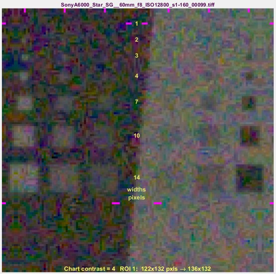
Object visibilityThe LARGE option covers both the upper and lower plot areas for improved visibility. Predicting object visibility for small, low contrast squares or 4:1 rectangles is the goal of SNRi measurements. The SNRi prediction begs for visual confirmation. We have developed a display for Imatest that does this with the contents of a real slanted-edge image and a bit of trickery. This display is different from most other Imatest displays in that it is intended for perceptual judgment, based on the original image (it’s hard to make perceptual judgments on slanted edges) and the calculated Line Spread Function (transformed into 2D). The results on the right are for a noisy image from a Micro Four-Thirds camera at ISO 12800. The sides of the squares are w = 1, 2, 3, 4, 7, 10, 14, and 20 pixels. The original chart had 4:1 contrast ratio (light/dark = 4), equivalent to a Michelson contrast CMich ((light-dark)/(light+dark)) of 0.6. The outer squares have CMich = 0.6, while the middle and inner squares have CMich = 0.3 and 0.15, respectively. How to use these images — Inconspicuous magenta bars near the margins are designed to help finding the small squares, which can be hard to see. The SNRi curves are (initially, at least) for the chart contrast — with 4:1 (the ISO 12233 standard) strongly recommended. The outer patches correspond to the SNRi curves, and according to the Rose theory, SNRi of 5 (14 dB) should correspond to the threshold of visibility. These can be compared with the SNRi curve. |
 |

Information capacity as a function of exposure (or Exposure Index)
The effects of exposure on information capacity C4 can be studied by running a batch of images in a fixed module (SFR, SFRplus, eSFR ISO, Checkerboard, or SFRreg), then entering the results (from a …-sfrbatch.csv file) into Batchview. Several steps are involved in getting good results. They can be done quickly, but it’s well-worth reading the instructions carefully.
This technique is most relevant to automotive cameras that need to work well in dim light. Exposure Index (EI) is used here as a substitute for total exposure. Increasing EI decreases the total light reaching the sensor, i.e., Exposure Index is inversely related to total exposure. (This can be confusing for beginners.)
We will work with a set of images from a 24 MP Micro Four-Thirds camera, exposed at different Exposure Indices (EIs; ISO speeds), acquired as raw (ARW), then converted with LibRaw to TIFF format with minimal processing: no sharpening or noise-reduction, and a simple gamma curve, but with white balance and color correction. JPEG files should be avoided if possible because their bilateral filtering reduces calculation accuracy. However, this may not be possible with automotive cameras, and fortunately the Edge Variance technique provides good results for C4 — just slightly less accurate than using a converted raw image.
The first step for the auto-ROI detection modules ( SFRplus, eSFR ISO, Checkerboard, or SFRreg) is to run an image through an interactive (Rescharts) version of the program to make sure settings are correct. This isn’t strictly necessary for SFR, but it can be useful, if only to preview the results.
Summary
- Shannon information capacity C has long been used as a measure of the goodness of electronic communication channels. It specifies the maximum rate at which data can be transmitted without error if an appropriate code is used (it took nearly a half-century to find codes that approached the Shannon capacity). Coding is not an issue with imaging. Rodney Shaw’s paper from 1962 [10] is a particularly good example of measuring C for photographic film— it wasn’t easy back then.
- C is ordinarily measured in bits per pixel. The total capacity is \( C_{total} = C \times \text{number of pixels}\).
- Because C is a function of MTF, the channel must be linearized before C is calculated, i.e., an appropriate gamma correction (signal = pixel level gamma, where gamma ≅ 2.2 for images in standard color spaces such as sRGB or Adobe RGB) must be applied to obtain correct values of S and N. The value of gamma (close to 2) can be determined from runs of any of the Imatest modules that analyze grayscale step charts: Stepchart, Colorcheck, Color/Tone, Multitest, SFRplus, or eSFR ISO. But in most cases it can be determined from the edge image if the chart contrast is entered and Use for MTF is checked.
- We hypothesize that C can be used as a figure of merit for evaluating camera quality, especially for machine vision and Artificial Intelligence cameras. (It doesn’t directly translate to consumer camera appearance because they have to be carefully tuned to reach their potential, i.e., to make pleasing images). It provides a fair basis for comparing cameras, especially when used with images converted from raw with minimal processing.
- Imatest calculates the Shannon capacity C for the Y (Luminance) channel of digital images, which approximates the eye’s sensitivity. It also calculates C for the individual R, G, and B channels as well as the Cb and Cr chroma channels (from YCbCr).
- Shannon capacity is unfamiliar in imaging because it was difficult to calculate and interpret. But now that it can be calculated easily, its relationship to photographic image quality is open for study.
- Since C is a new measurement, we are interested in working with companies or academic institutions who can verify its suitability for Machine Vision and Artificial Intelligence systems.
|
Note: A slanted-edge information capacity measurement used prior to Imatest 2020, used primarily to obtain total information capacity from Siemens star measurements, has been deprecated completely because it was not sufficiently accurate. |
Links (more links in the White Paper)
- C. E. Shannon, “A mathematical theory of communication,” Bell Syst. Tech. J., vol. 27, pp. 379–423, July 1948; vol. 27, pp.
623–656, Oct. 1948. - C. E. Shannon, “Communication in the Presence of Noise”, Proceedings of the I.R.E., January 1949, pp. 10-21.
- Wikipedia – Shannon Hartley theorem has a frequency dependent integral form of Shannon’s equation that is applied to both Imatest’s sine pattern and slanted edge Shannon information capacity calculation.
- I.A. Cunningham and R. Shaw, “Signal-to-noise optimization of medical imaging systems”, Vol. 16, No. 3/March 1999/pp 621-632/J. Opt. Soc. Am. A
- Brian W. Keelan, “Imaging Applications of Noise Equivalent Quanta” in Proc. IS&T Int’l. Symp. on Electronic Imaging: Image Quality and System Performance XIII, 2016, https://doi.org/10.2352/ISSN.2470-1173.2016.13.IQSP-213.
- Michail C, Karpetas G, Kalyvas N, Valais I, Kandarakis I, Agavanakis K, Panayiotakis G, Fountos G., Information Capacity of Positron Emission Tomography Scanners. Crystals. 2018; 8(12):459. https://doi.org/10.3390/cryst8120459.
- Christos M. Michail, Nektarios E. Kalyvas, Ioannis G. Valais, Ioannis P. Fudos, George P. Fountos, Nikos Dimitropoulos, Grigorios Koulouras, Dionisis Kandris, Maria Samarakou, Ioannis S. Kandarakis, “Figure of Image Quality and Information Capacity in Digital Mammography”, BioMed Research International, vol. 2014, Article ID 634856, 11 pages, 2014. https://doi.org/10.1155/2014/634856.
- Paul J. Kane, “Signal detection theory and automotive imaging”, Proc. IS&T Int’l. Symp. on Electronic Imaging: Autonomous Vehicles and Machines Conference, 2019, pp 27-1 – 27-8, https://doi.org/10.2352/ISSN.2470-1173.2019.15.AVM-027.
- Orit Skorka, Paul J. Kane, “Object Detection Using an Ideal Observer Model”, IS&T Int’l. Symp. on Electronic Imaging: Autonomous Vehicles and Machines, 2020, pp 41-1 – 41-7, https://doi.org/10.2352/ISSN.2470-1173.2020.16.AVM-041.
- R. Shaw, “The Application of Fourier Techniques and Information Theory to the Assessment of Photographic Image Quality”, Photographic Science and Engineering, Vol. 6, No. 5, Sept.-Oct. 1962, pp.281-286. Reprinted in “Selected Readings in Image Evaluation,” edited by Rodney Shaw, SPSE (now SPIE), 1976. A fascinating and difficult calculation of information capacity of photographic film. Available for download
- X. Tang, Y. Yang, S. Tang, Characterization of imaging performance in differential phase contrast CT compared with the conventional CT: Spectrum of noise equivalent quanta NEQ(k), Med Phys. 2012 Jul; 39(7): 4467–4482. Published online 2012 Jun 29. doi: 10.1118/1.4730287.
Appendix 1. Concise summary of information capacity
Claude Shannon
Nothing like a challenge! There is such a metric for electronic communication channels— one that quantifies the maximum amount of information that can be transmitted through a channel without error. The metric includes sharpness and noise (grain in film). And a camera— or any digital imaging system— is such a channel.
The metric, first published in 1948 by Claude Shannon* of Bell Labs [1,2], has become the basis of the electronic communication industry. It’s called the Shannon channel capacity or Shannon information capacity C, and has a deceptively simple equation [3]. (See the Wikipedia page on the Shannon-Hartley theorem for more detail.)
\(\displaystyle C = W \log_2 \left(1+\frac{S}{N}\right) = W \log_2 \left(\frac{S+N}{N}\right) = \int_0^W \log_2 \left( 1 + \frac{S(f)}{N(f)} \right) df\)
W is the channel bandwidth, S(f) is the average signal energy (the square of signal voltage; proportional to MTF(f)2), and N(f) is the average noise energy (the square of the RMS noise voltage), which corresponds to grain in film. It looks simple enough (only a little more complex than E = mc2 ), but it’s not easy to apply.
*Claude Shannon was a genuine genius. The article, 10,000 Hours With Claude Shannon: How A Genius Thinks, Works, and Lives, is a great read. There are also a nice articles in The New Yorker and Scientific American. And IEEE has an article connecting Shannon with the development of Machine Learning and AI. The 29-minute video “Claude Shannon – Father of the Information Age” is of particular interest to me it was produced by the UCSD Center for Memory and Recording Research. which I frequently visited in my previous career.
This page describes how information capacity C is calculated from images of slanted-edges, Imatest’s most widely-used test image, and how to signal and noise are calculated from the same location, resulting in a superior measurement of image quality. An earlier (2020) Siemens star method is described in Shannon information capacity from Siemens stars.
The math and algorithms behind the calculations are presented in Information capacity measurements from Slanted edges: Equations and Algorithms.
Appendix 2. Calculating maximum information capacity, Cmax, for linear sensorsStep1: Replace the measured peak-to-peak voltage range Vp-p with the maximum allowable value, Vp-p_max = 1, This may seem like a simplification, but it works well for most cameras. Referring to the section on Signal Power S, Step 2: Replace the measured noise power N with Nmean, the mean of N over the range 0 ≤ V ≤ 1 (where 1 is the maximum allowable normalized signal voltage V). The general equation for noise power N as a function of V for linear image sensors is \(\displaystyle N(V) = k_0 + k_1V\) k0 is the coefficient for constant noise (dark current noise, Johnson (electronic) noise, etc.). k1 is the coefficient for photon shot noise. They are calculated from noise powers N1 = σ12 and N2 = σ22, which are measured along with signal voltages V1 and V2 on either side of the edge transition. Assuming N1 = k0+ k1V1 and N2 = k0+ k1V1 , we can solve two equations in two unknowns for k0 and k1. \(\displaystyle k_0 = \frac{N_1V_2-N_2V_1}{V_2-V_1} ; \ \ \ k_1=\frac{N_2-N_1}{V_2-V_1}\) N closely approximates the noise used in noise calculation method (1) (used for minimally-processed images that don’t have bilateral filtering). But if method (2) (the smoothed peak noise) is used (recommended for in-camera JPEGs with bilateral filtering), N is generally larger, and must be modified. N → kNN, where kN = Nmethod_2 / NMethod_1 In bilateral-filtered images (most JPEGs from consumer cameras), lowpass filtering (for noise reduction) may be affect N1 and N2 strongly enough so the equation does not reliably hold. This can adversely affect the accuracy of Cmax. The mean noise power Nmean over the range 0 ≤ V ≤ 1 for calculating Cmax is \(\displaystyle N_{mean} = \frac{\int_0^1 N(V) d\nu}{\int_0^1 d\nu} = \int_0^1 (k_0 + k_1V) d\nu = k_0+k_1/2\) To handle the rare, but not unknown, cases where noise is larger for the dark side of the edge (weird image processing), use Nmean = max(Nmean,N1,N2). Using \(N = N_{mean}, \ \ V_{p-p\_max} – 1 \text{ and } S_{avg}(f) = MTF(f)^2/12,\) , \(\displaystyle C_{max} = \int_0^{0.5} \log_2 \left( 1+\frac{MTF(f)^2}{12\ N_{mean}} \right) df \cong \sum_{i=0}^{0.5 / \Delta f} \log_2 \left(1+\frac{MTF(i\ \Delta f)^2}{12\ N_{mean}} \right) \Delta f\) Because noise in High Dynamic Range (HDR) sensors does not follow the simple equation for linear sensors, we recommend giving the image sufficient exposure so the brighter side of the edge is close to (but definitely below) saturation, then leaving N unchanged (Nmean = N). Cmax is nearly independent of exposure for minimally or uniformly-processed images with linear sensors, where noise power N is a known function of signal voltage V. |
Appendix 3: JSON output
Obtained by saving JSON summary file (press Save data in Rescharts)
Notes
“edge_info_note1”: “Information capacity results. For color images, channels are R G B Y; R GR B GB for Bayer”,
“edge_info_note2”: “V_P_P and following results contain nroi results for one color per line”,
The following results have 4 Rows for RGBY channels; 6 Columns for the 6 ROIs.
Signal VP-P
“edge_info_signal_V_P_P”: [
[0.2271,0.2283,0.2199,0.2125,0.1971,0.1887],
[0.2292,0.2302,0.2209,0.2157,0.1994,0.1889],
[0.2358,0.2354,0.2239,0.1998,0.2075,0.1886],
[0.2292,0.2301,0.2209,0.2138,0.1995,0.1889]
],
Mean spatially dependent noise
“edge_info_noise_V_RMS”: [
[0.0062,0.0061,0.0056,0.0057,0.0059,0.0064],
[0.006,0.006,0.0054,0.0059,0.0058,0.0065],
[0.0061,0.0063,0.0062,0.007,0.0062,0.0076],
[0.0058,0.006,0.0052,0.0058,0.0058,0.0064]
],
Peak smoothed noise
“peak_smoothed_noise”: [
[0.0149,0.0179,0.0137,0.0151,0.0172,0.0128],
[0.015,0.0177,0.0132,0.0151,0.0172,0.0131],
[0.0156,0.0185,0.0146,0.016,0.0181,0.0134],
[0.0151,0.0178,0.0132,0.0151,0.0172,0.0129]
],
Peak smoothed noise/mean noise ratio: used to detect bilateral filtering when above threshold (1.8*max(mean on left, mean on right)).
“pk_smoothed_to_mean_noise_ratio”: [
[2.413,2.922,2.449,2.637,2.933,2.02],
[2.508,2.946,2.455,2.554,2.985,2.018],
[2.573,2.953,2.343,2.296,2.917,1.76],
[2.576,2.972,2.525,2.607,2.996,2.009]
],
Standard deviation of detected location in pixels (σ(location))
“sigma_location_pxls”: [
[0.068,0.085,0.126,0.129,0.124,0.112],
[0.068,0.083,0.12,0.128,0.123,0.113],
[0.069,0.084,0.129,0.144,0.123,0.114],
[0.068,0.083,0.12,0.128,0.123,0.112]
],
Signal/Noise RMS (we are not sure of the purpose of this measurement; may not be kept.)
“edge_info_snr_RMS”: [
[12.9707,13.1877,13.8628,13.1201,11.8556,10.5008],
[13.5087,13.509,14.5215,12.8755,12.2126,10.3129],
[13.7273,13.286,12.6874,10.1264,11.821,8.7738],
[13.8613,13.6161,14.9063,13.0611,12.2589,10.3593]
],
Edge variance information capacity C_4
“edge_info_capacity_C_4_b_p”: [
[2.031,1.651,1.231,1.167,1.148,2.201],
[2.032,1.671,1.27,1.175,1.16,2.179],
[2.023,1.654,1.198,1.076,1.144,1.983],
[2.031,1.67,1.269,1.172,1.16,2.185]
],
Edge variance information capacity C_max
“edge_info_capacity_C_max_b_p”: [
[4.032,3.471,2.737,3.166,2.926,4.023],
[4.005,3.501,2.86,3.023,3.084,3.976],
[4.032,3.495,2.62,2.924,2.916,3.724],
[4.044,3.513,2.876,3.112,3.038,3.982]
],
C_4 from Noise image (NEQ) info_capacity… replaces edge_info_capacity…
“info_capacity_C_4_NEQ_b_p”: [
[2.128,1.567,1.056,0.8549,1.097,2.254],
[1.973,1.544,0.9904,0.9072,1.073,2.279],
[1.883,1.614,1.058,1.075,1.036,2.382],
[1.875,1.526,0.9486,0.8741,1.046,2.262]
],
C_max from Noise image info_capacity… replaces edge_info_capacity…
“info_capacity_C_max_NEQ_b_p”: [
[4.128,3.387,2.562,2.854,2.874,4.076],
[3.947,3.374,2.58,2.756,2.997,4.075],
[3.891,3.455,2.48,2.923,2.808,4.122],
[3.888,3.368,2.556,2.814,2.925,4.059]
],
Number of images averaged ([1] indicates no signal averaging)
“signal_averages_for_info”: [1],
Total maximum information capacity in Mb (all ROIs). Shown in 3D plot for C_max.
“edgeInfoCapacityMax_total_Mb”: [23.39],
Section indicator for individual regions, showing the selected channel.
“edge_info”: {
“channels”: “Y”,
Frequencies (cycles/pixel shown) for NPS and NEQ, below. 0 and 0.05 to 0.5 in steps of 0.05.
“NPS_NEQ_frequency”: [0,0.05,0.1,0.15,0.2,0.25,0.3,0.35,0.4,0.45,0.5],
Widths in pixels for SNRi and Edge SNRi (the shorter dimension for a 4:1 rectangle)
“SNRi_box_width”: [20,14,10,7,5,4,3,2.5,2,1.4,1,0.7,0.5],
Results for individual regions, indicated by “ROI” Only 2 of several are shown.
ROI indicates the region.
Noise power spectrum (NPS)
Noise Equivalent Quanta (NEQ)
SNRI_square. All SNRis for box widths from 20 to 0.5.
SNRi_rectangle
edge_SNRi_square. Replace SNRd_square – an obsolete designation prior to the 24.2 pilot program.
edge_SNRi_rectangle Replaces SNRd_rectangle – an obsolete designation
“ROI_results”: [
{
“ROI”: [1],
“noise_power_spectrum”: [0.002352,0.000627,0.0005093,0.0003993,0.0003269,0.0003086,0.0002547,0.0001938,0.0001532,0.0001075,6.15e-05],
“noise_equivalent_quanta”: [28.98,110.9,170.2,279.3,357.6,317.5,274.2,215.5,147.9,111.9,106.6],
“SNRi_square”: [42.16,39.41,37.03,34.55,32.22,30.79,28.8,27.34,25.33,21.34,16.72,11.21,5.705],
“SNRi_rectangle”: [49,45.79,43.04,40.28,37.78,36.27,34.35,33.03,31.29,28,24.36,20.06,15.67],
“SNRd_square”: [12.01,11.98,11.99,11.91,11.89,12.12,12.16,12.27,12.77,11.47,8.007,3.074,-2.18],
“SNRd_rectangle”: [12.01,11.98,11.98,11.95,11.94,12.08,12.08,12.2,12.46,11.98,10.5,8.153,5.667]
},
{
“ROI”: [2],
“noise_power_spectrum”: [0.003468,0.0009693,0.0005746,0.0004773,0.0004368,0.0003866,0.0003348,0.0002759,0.0002067,0.0001327,7.788e-05],
“noise_equivalent_quanta”: [19.9,72.8,153.7,221.5,242.4,217.2,161.5,104.6,64.98,43.74,36.32],
“SNRi_square”: [40.71,37.97,35.44,32.97,30.72,29.25,27.2,25.68,23.53,19.28,14.49,8.887,3.331],
“SNRi_rectangle”: [47.58,44.41,41.53,38.73,36.28,34.77,32.8,31.45,29.63,26.18,22.42,18.04,13.54],
“SNRd_square”: [9.553,9.552,9.528,9.504,9.501,9.651,9.914,10.1,10.18,8.332,4.651,-0.3857,-5.685],
“SNRd_rectangle”: [9.553,9.547,9.538,9.521,9.523,9.614,9.748,9.894,9.992,9.23,7.584,5.199,2.496]
…
},
]
},