Imatest eSFR ISO results
Imatest eSFR ISO performs highly automated measurements of several key image quality factors using one of three versions of the ISO 12233:2017 Edge SFR chart: Standard, Enhanced, or Extended or the Extended ISO 12233:2023 . Unlike most other modules, the user never has to manually select Regions of Interest (ROIs). Image quality factors include
- Sharpness, expressed as Spatial Frequency Response (SFR), also known as the Modulation Transfer Function (MTF),
- Noise, measured from the grayscale patches surrounding the center of the chart, includes all types of noise calculated by Color/Tone Interactive and Color/Tone Auto (standard pixel noise, chroma noise, scene-referenced noise, sensor (raw) noise, and ISO-15739 visual noise). SNR (Signal-to-Noise Ratio) can also be displayed as a ratio or in dB.
- Lateral Chromatic Aberration,
- Distortion (with nearly as detailed output as the Distortion module). Described in detail here.
- Tonal response (again, with less detail than Stepchart; no noise statistics)
- Color accuracy, when used with an eSFR ISO chart that contains the color pattern.
- ISO sensitivity (Saturation-based and Standard Output Sensitivity), when incident lux is entered.
This document illustrates eSFR ISO results. Part 1 introduced eSFR ISO and explained how to obtain and photograph the chart. Part 2 showed how to run eSFR ISO inside Rescharts and how to save settings for automated runs.
eSFR ISO results
When calculations are complete, results are displayed in the Rescharts window, which allows a number of displays to be selected. The following table shows where specific results are displayed.
 eSFR ISO display selections
| Measurement | Display |
| MTF (sharpness) for individual regions | 1. Edge and MTF |
| MTF (sharpness) for entire image | 4. Multi-ROI summary 12. 3D plot 13. Lens-style MTF plot |
| Lateral Chromatic Aberration | 2. Chromatic Aberration |
| Distortion, misalignment, Field of View, Original image showing region selection |
8. Image & geometry |
| Distortion | 16. Radial Distortion Plot |
| Tonal response & gamma | 5. Tonal response & gamma |
| Noise | 6. Histograms and noise stats |
| Color accuracy | 10. a*b* Color error 11. Split colors |
| ISO Sensitivity | 5. Tonal response & gamma |
| EXIF data | 7. Summary & EXIF data |
| SQF (Subjective Quality Factor)/Acutance | 3. SQF / Acutance |
| Edge roughness | 14. Edge roughness |
| Chromatic Aberration (radial) | 15. Radial (Chr Aber, etc.) |
| Distortion (radial) | 16. Radial Distortion plot |
| Noise (several flavors) | 17. Noise (eSFR ISO-only) |
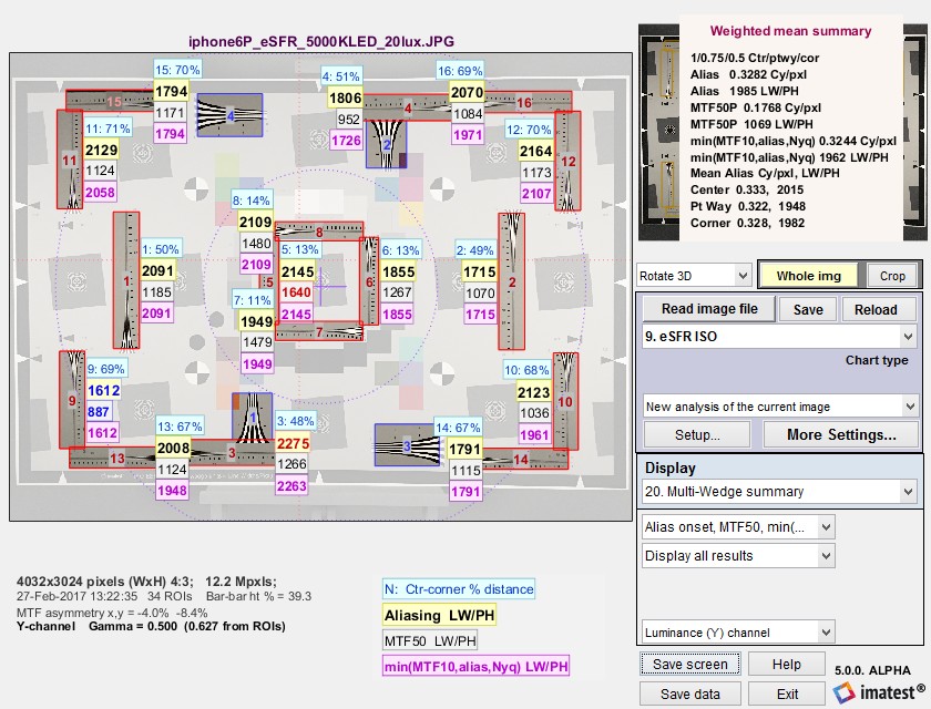
Multi-ROI summary display
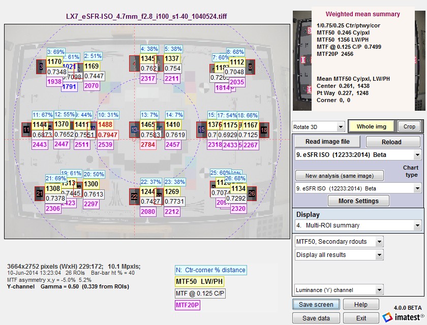 eSFR ISO results in Rescharts window: Multiple region (ROI) summary
|
The multi-ROI (multiple Region of Interest) summary shown in the Rescharts window (above) contains a detailed summary of eSFR ISO results. (3D plots also contain an excellent summary.) The upper left contains the image in muted gray tones, with the selected regions surrounded by red rectangles and displayed with full contrast. Up to four results boxes are displayed next to each region. The results depend on the the Display options area on the right, below the Display selection. There is a legend below the image. The approximate location of maximum MTF, based on a second order fit to MTF results, is indicated by a red ‘O’ at the intersection of vertical and horizontal dotted lines (– – – – O – – – –). |
 Results selection |
 View selection View selection |
| The Results selection (right) lets you choose which results to display. N is region number. Ctr-corner distance % is the approximate location of the region. CA is Chromatic Aberration in area, as percentage of the center-to-corner distance (a perceptual measurement). | ||
| The View selection (far right, above) lets you select how many results boxes to display, which can be helpful when many regions overlap. From top to bottom the number of boxes is 4, 3, 2, 2, and 1, respectively. | ||
Distortion statistics, shown in the lower left, are described in detail in SFRplus Distortion and Field of View Measurements.
- SMIA TV distortion is the simplest overall measure of distortion. it is positive for pincushion distortion and negative for barrel distortion.
- k1 (the third order distortion coefficient). ru = rd + k1 rd3 = where ru is the undistorted radius and rd is the distorted radius. r is normalized to the center-to-corner distance. k1 > 0 for barrel distortion and k1 < 0 for pincushion.
Arctangent/tangent distortion coefficients (used in Picture Window Pro) are also calculated and included in the CSV output file.
MTF asymmetry is calculated in the x (horizontal) and y (vertical) directions. MTF50 as functions of x and y are fitted to second-order (parabolic) curves, which are used to calculate expected MTF50 values at the Top, Bottom, Left and Right (MTF50T, etc.) of the image.
MTF asymmetry (x) = (MTF50R-MTF50L) / (MTF50R+MTF50L)
MTF asymmetry (y) = (MTF50T-MTF50B) / (MTF50T+MTF50B)
Weighted summary results are displayed on the upper-right. The default weights are 1.0 for ROIs in the central region (inside the inner dotted circle), 0.75 for the middle region (between the two dotted circles), and 0.5 for the outer region (outside the outer dotted circle). These weights can be changed in the eSFR ISO Settings window. The results are independent of the number of ROIs in each region.
Plot settings area
A small number of options are available in the Plot settings area, on the lower right, below the Display box (fewer than for other Rescharts modules).
All displays contain the dropdown menu for selecting the primary channel to analyze. If R, G, B, or Y (Luminance) is selected, all channels are analyzed, but the selected channel is emphasized. There is also an option to analyze any of the channels alone— useful where one of the secondary channels is dark and may cause a run to crash. Luminance (Y) is shown above. If it is changed, results are recalculated.
Many displays allow you to select the ROI for viewing results.
The Edge and MTF display has a dropdown window for selecting the maximum MTF display frequency: 2x Nyquist (the default), Nyquist, 0.5x Nyquist, and 0.2x Nyquist.
Edge and MTF display
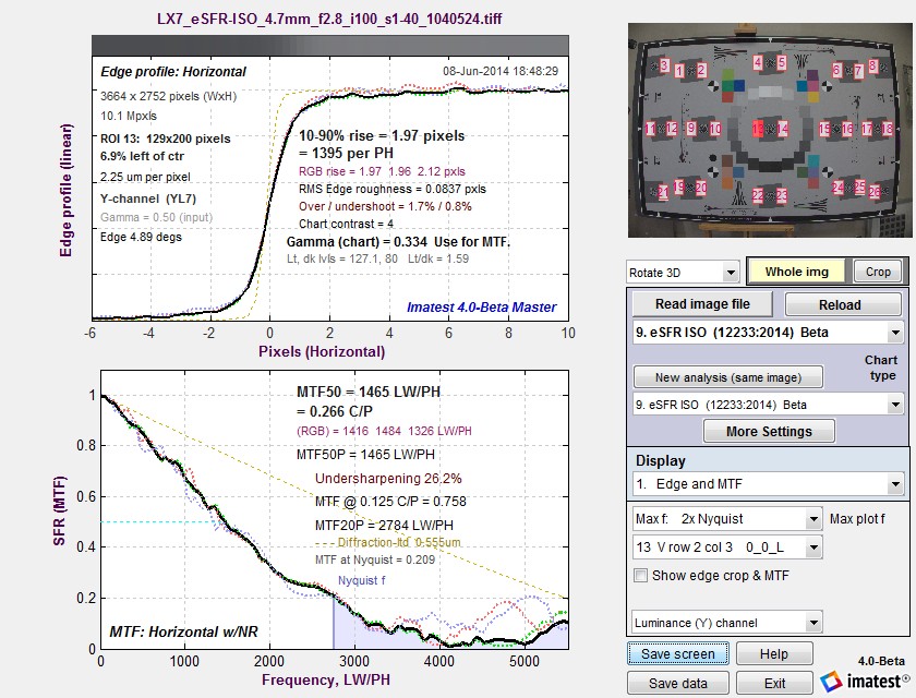
Edge and MTF display in Rescharts window
Diffraction-limited MTF and edge response are shown as a pale brown dotted lines
when pixel spacing has been entered.
This display is identical to the SFR Edge and MTF display. The edge (or line spread function) is plotted on the top and the MTF is plotted on the bottom. The edge may be displayed linearized and normalized (the default; shown), unlinearized (pixel level) and normalized, or linearized and unnormalized (good for checking for saturation, especially in images with poor white balance). Edge display is selected by pressing .
There are a number of readouts, including 10-90% rise distance, MTF50, MTF50P (the spatial frequency where MTF is 50% of the peak value, differing from MTF50 only for oversharpened pulses), the secondary readouts (MTF30 and MTF@30 lp/mm in this case), and the MTF at the Nyquist frequency (0.5 cycles/pixel). The diffraction-limited MTF curve is displayed as a pale brown dotted line.
MTF is explained in Sharpness: What is it and how is it measured? MTF curves and Image appearance contains several examples illustrating the correlation between MTF curves and perceived sharpness.
An important (and optional) readout in the upper plot is
- The Chart contrast (entered in the Display options section of the eSFR ISO settings window),
- The Contrast factor: the ratio between the chart contrast derived from the pixel ratio and the input value of gamma (0.5 in the above display),
- Gamma (from chart): a measurement of gamma derived from the chart pixel levels and the Chart contrast (an input value, as described above). Gamma has a relatively small effect on the MTF measurement, especially for moderate to low contrast targets (10:1 or under).
Chromatic Aberration
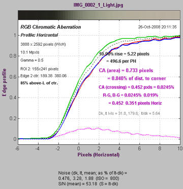
Lateral Chromatic Aberration
Lateral Chromatic Aberration (LCA), also known as “color
fringing,”
is most visible on tangential boundaries near the edges of the image. Much of the plot is grayed out if the selected region (ROI) is too close to the center (less than 30% of the distance to the corner) to accurately measure CA.
The area between the highest and lowest of the edge curves (shown for the R, G, B, and Y (luminance) channels) is a perceptual measurement of LCA. It has units of pixels because the curves are normalized to an amplitude of 1 and the x-direction (normal to the edge) is in units of pixels. It is displayed as a magenta curve.
Perceptual LCA is also expressed as percentage of the distance from center to corner, which tends to be more reflective of system performance: less sensitive to location and pixel count than the pixel measurement. Values under 0.04% of the distance from the center are insignificant; LCA over 0.15%
can be quite visible and serious.
Information for correction LCA (R-G and B-G crossing distances) is also given in units of % (center-to-corner) and pixels. LCA can be corrected most effectively before demosaicing. Results are explained in Chromatic Aberration … plot.
SQF (Subjective Quality Factor)
|
SQF is a perceptual measurement of the sharpness of a display (monitor image or print). MTF, by comparison is device sharpness (not perceptual sharpness). SQF includes the effects of the human visual system’s Contrast Sensitivity Function (CSF), print (or display) size, and viewing distance (which is assumed to be proportional to print height, by default). SQF is available when Speedup is unchecked in the input dialog box. See Introduction to SQF for more detail.
|
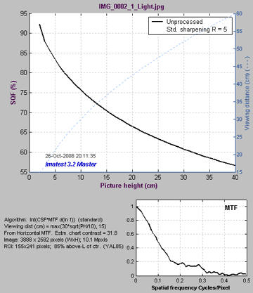 SQF (Subjective Quality Factor) |
Tonal response & gamma
|
This display is derived from the 20-patch ISO 14524 stepchart pattern, located in the center of the eSFR ISO test chart. It resembles the third figure in Stepchart. The upper plot shows the tonal response (also called OECF for Opto-Electronic Conversion Function) for all colors. The lower plot shows instantaneous gamma— the slope (derivative) of tonal response. The value of gamma may differ slightly from the values in the Edge response and MTF display because it’s calculated differently– based on the average slope of the light to middle tone squares of the stepchart. The levels of the light and dark portions of the patches used to calculate MTF are shown as pale horizontal lines and as points on the extreme left and right of the upper plot. You can use these lines to see if the patches are within the (relatively) linear region of tonal response (they are in the example on the right). A warning message (Warning: MTF patches may saturate ) is displayed if any of the patches are close to saturation (log(pixel level/255) > -0.01; roughly, pixel level > 249 of 255).
|
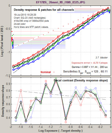 Tonal response & gamma Tonal response & gamma |
Histograms and noise analysis
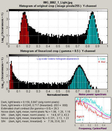
Histograms and noise stats
This display, available when Speedup is unchecked, contains histograms of pixel levels for individual ROIs (original on top and linearized using input gamma on bottom). Since this slows calculations considerably, we only recommend unchecking Speedup when histograms are needed (which will be infrequently).
The black (background) histogram contains pixel levels for the entire ROI. The red histogram is for the right (dark) region, away from the transition, used in the noise statistics calculation. The cyan histogram is for the left (light) region. Sharpening may cause extra bumps to appear in the black histogram. A detailed level and noise analysis is displayed below the image.
| Dark, light levels | Original pixel levels normalized to 1 and linearized levels, also normalized to 1 |
| Estimated chart contrast (for gamma = …) | The correct chart contrast must be entered in eSFR ISO Setup window. |
| Noise (dark, light, mean; norml pixels %) | RMS noise expressed in pixels, normalized to 100% (for 255 in 8-bit files) |
| S/N (…; norml pixels) | Signal/Noise, where signal is mean pixel level of ROI at a distance from the transition. |
| Noise (…; linearized %) | Noise, linearized using gamma (input); normalized to 100% |
| S/N (…; linearized) | Signal/Noise, linearized |
Noise calculations are made in portions of the ROIs (Regions of Interest) away from the transitions. They are facilitated by selecting wide ROIs. The noise spectrum on the lower right contains qualitative information about noise visibility and software noise reduction, which generally reduces high frequency noise below 0.5, typical of demosaicing alone. The region on the right is shown in red; left is shown in cyan. See also Noise.
Image, Geometry, Distortion, FoV
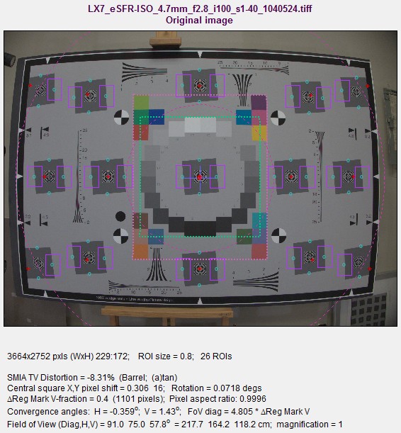 Image, Geometry, Distortion, FoV display
This display allows several aspects of the image to be viewed in detail. It shows the selected regions for MTF/noise analysis (violet rectangles), the yellow rectangles used for generating the uniformity profiles, and the red horizontal curves used to measure distortion). Display options include
| Original Image | Extreme Lighten (HSL) |
| Rec channel | Lighten (HSV) |
| Green channel | Lighten 1 bit |
| Blue channel | Lighten 2 bits |
| Color: Boost Sat. 4X | Original w/5×5 grid |
| Color: Boost Sat, 10X | Original w/5×7 grid |
| Lighten (HSL) | Original w/11×15 grid |
A number of geometrical results are shown beneath the image. Distortion results are described in more detail in SFRplus Distortion and Field of View measurements
- WxH of image in pixels; m x n squares found; ROI size (referencing input setting), number of ROIs for MTF, etc. (not for profiles).
- SMIA TV Distortion: Barrel (0)
- 3rd order, 5th order, and arctan/tan distortion coefficients The best of these (with the least optimizer error) may be used to find Field of View.
- x,y coordinates of the center of the middle square relative to the image center.
- The average rotation of the pattern in degrees (>0 for clockwise)
- The bar-to-bar vertical height as a fraction of the image height and in pixels.
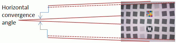
- Convergence angles (degrees). These are the result of perspective distortion, when the camera is not pointed directly at the target or is misaligned. The horizontal convergence angle (related to yaw) is shown below: calculated by extrapolating the horizontal bars to the top and bottom. A positive angle has a vortex to the left. In the illustration below the pairs of solid red lines at the top and bottom are parallel (to fit the image on the page).
Perfect alignment would be x,y coordinates, rotation, and H,V convergence = 0. Vertical and Horizontal convergence angles are calculated from the registration marks, extrapolated to the image edges. With fisheye (strongly barrel-distorted) lenses the chart must be precisely centered for the convergence angle measurement to be meaningful.
- measured focal length of the lens is displayed when Registration mark vertical spacing in cm, Lens-to-chart distance in cm, and Pixel spacing (pitch) have been been entered. It is written to the CSV output file if calculated. Equations: Magnification M is registration mark spacing (on the sensor) / registration mark spacing (on the chart). For Lens-to-chart distance f1, lens-to-sensor distance f2 = f1M. Using the thin lens equation, focal length f = 1/(1/ f1+1/ f2).
- Field of view calculations include the effects of distortion (the best of 3 models is used). FoV in centimeters (cm) is displayed if the bar-to-bar vertical distance (in the chart center for pre-distorted charts) is entered. FoV in degrees is displayed if the lens-to-chart distance in cm is also entered.
A particularly interesting display is available when you click Crop to ROI (or Crop to 1/2 ROI). This display is also available in the Edge and MTF display shen you click the Show edge crop & MTF checkbox. The ROI is displayed large enough so its blur is clearly visible and can be compared with Edge and MTF plots and summary results.
 Image, Geometry, Distortion, FoV display, showing Crop to ROI, which allows
the edge appearance (enlarged) to be compared to Edge and MTF results.
Summary & EXIF data
|
This plot contains summary results for individual ROIs and EXIF data (metadata that describes camera and lens settings). When first installed, Imatest reads EXIF data from JPEG files only. Enhanced EXIF support requires a special download of ExifTool, described here. EXIF data may be viewed at any time from any display by clicking File, View All EXIF Data.
|
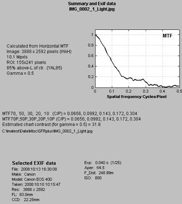 Summary & EXIF data |
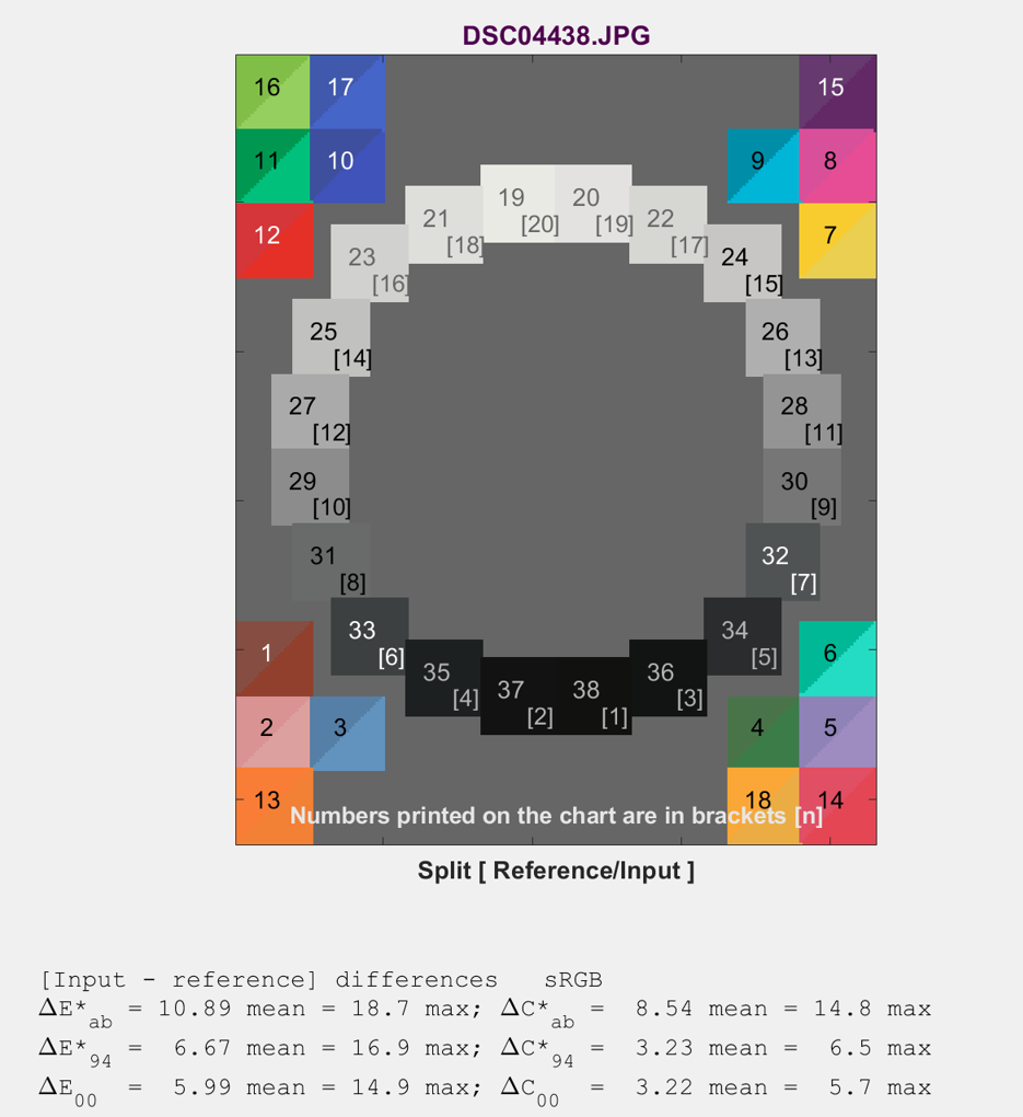
Color analysis
|
A color analysis is available for images that contain the eSFR ISO color pattern (available when the media, i.e., inkjet and LVT on color film, allows), which consists of 16 colors that are close to 16 of the 18 colors of the industry-standard 24-patch color chart. To obtain a color analysis,
Two displays are available in the color analysis. The a*b* color error display, shown on the right, is similar to displays in Colorcheck and Color/Tone Interactive. This display shows the reference (nominal) {a*,b*}values as squares and the camera (measured) values as circles. Normally the mean and maximum values of ΔE*ab, ΔC*ab, ΔE*94, ΔC*94, ΔE*00 and ΔC*00 are displayed.
The Split (Reference/Input) display is shown on the right. The bottom shows statistics for the red patch in Row 3, left, obtained by clicking in the Display area on the lower right (not shown). To turn off the probe, click outside the image (in the current version, you need to click on the text below the image.) When the Probe is off the mean and maximum values of ΔE*ab, ΔC*ab, ΔE*94, ΔC*94, ΔE*00 and ΔC*00 are displayed. Patch order: |
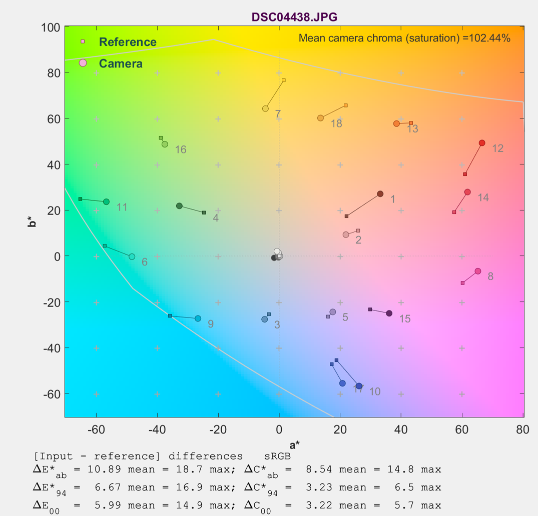 a*b* color error
|
3D Plots
|
Displays results as three-dimensional pseudocolor images. The parameter to be displayed is selected by Plot options, shown on the right. (Only MTF50, automatically scaled, can be displayed in Imatest Studio) The display can be rotated for enhanced visualization. Region selection should include at least 13 regions. A 5x5 ROI grid (23 regions) was chosen for the analysis on the right. The largest selection that avoids the low contrast edges, which tend to have lower MTFs in typical consumer/DSLR cameras with nonlinear signal processing, is 13. All sqs, inner & bdry except low contrast. Single-contrast charts (without the low contrast regions) work well for 3D plots (for example, in equipment reviews). The rather strangely shaped surface (center has lower MTF than part way region) may be the result of autofocus issues and/or curvature of field. Several Display options are available. The Pseudocolor shaded plot with image and text shown on the right is the most generally useful. Other options include no shading, colored contour lines-only, and 3D plots only (displayed larger, but without the summary image and text shown below the 3D plot).
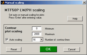
Display area. Details on right The Z-axis of the image (which contains the results) can be inverted to reveal detail obscured in a normal display. The background color can be varied from white to black using the Backgnd slider. The default is light gray (0.9). Manual or automatic scaling may be selected in Master using the button. Automatic is the default. When is pressed, the Manual scaling window, shown on the right, lets you set the scaling for the parameter selected in the Plot menu (MTF50P in this case). Minimum and Maximum only apply for manual scaling, i.e., when Auto scaling is unchecked. 6, 11, 16, 21, or 26 contour lines may be selected. The button sets a top (pseudo-2D) view. It toggles between and . You can rotate the image starting from either setting. Several 3D plots can be displayed in eSFR ISO Auto by making appropriate selections in the button in the eSFR ISO settings window. |
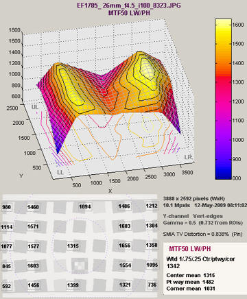
MTF50 3D plot
Scaling window |
Lens-style MTF plot
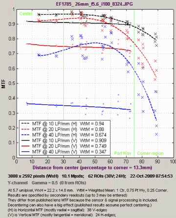
Lens-style MTF plot
Produces results similar to the MTF plots in the Canon (explanation), Nikon (explanation), and Zeiss websites. Up to three plot parameters may be selected with the Secondary readout. Typical choices are MTF at 10, 20, and 40 lp/mm (used by Zeiss) or 10 and 30 lp/mm (used by Canon and Nikon). Pixel spacing (um/pixel, etc.) must entered to obtain lp/mm spatial frequencies.
A minimum of 13 regions is recommended, though more are better. 15. Ctrs, all is the recommended region setting. 13. Ctrs, all outer or 14. Ctrs, all inner also work. This plot is only recommended for enhanced or extended charts. V&H edges (both) should be selected.
Though these plots are similar to the website plots, there are several significant differences.
- Imatest calculates he system MTF, including the sensor and signal-processing. The websites display the optically-measured MTF for the lens-only. Imatest results are comparable, but never identical, to the published lens curves.
- The horizontal (H) MTF curves, derived from vertical edges, are mostly radial (sagittal) near the sides of the image (at large distances from the center). The SFRplus chart was designed for this purpose.
- The Vertical (V) MTF curves, derived from horizontal edges, are mostly tangential (meridional) near the sides.
- The published curves assume perfect centering. Some manufacturers, like Canon, obtain their results from design calculations, not from measured test results (no centering issues— or perhaps they use “cherry-picked” lenses!). Real lenses almost always exhibit some decentering, primarily due to manufacturing variability, which is more visible in other displays, particularly the 3D plots. In the lens-style MTF plot, decentering shows up as a spread in the individual readings (x for Horizontal MTF from vertical edges, • for Vertical MTF from horizontal edges).
The curves are calculated using third-order polynomial regression. With higher-order regression, scatter due to lens decentering often caused the curves to display serious irregularities.
Edge roughness plotAnalyzes edge roughness, which has two components:
The periodic noise has peak spectral response at spatial frequencies corresponding to one or two pixels perpendicular to the edge, where one pixel corresponds to the green channel and two pixels corresponds to the red and blue channels of Bayer color filter arrays. In the Roughness Spectrum (lower) plot these frequencies are 1 and 0.5, respectively. The response peaks at these frequencies are fairly typical. The periodic noise is calculated by transforming the frequency components at f = 0.5 through 2.5 in steps of 0.5 ( i.e., the aliasing fundamentals and the first few harmonics) back into spatial domain. The aperiodic noise is calculated by subtracting the periodic noise from the total noise. Three RMS (σ = standard deviation) roughness values are reported: Total, aliasing (jaggies), and Total-aliasing (aperiodic). The interpretation of edge roughness results is somewhat challenging because it’s a new measurement and there isn’t a lot of data for comparison. While the pattern on the right is fairly typical (and expected), we’ve seen many spectra that don’t resemble it at all. In general noise, peaks are weak (or nonexistent) for blurred edges. Although we hope this calculation will enable us to distinguish excellent and mediocre demosaicing algorithms, we’re not there yet. |
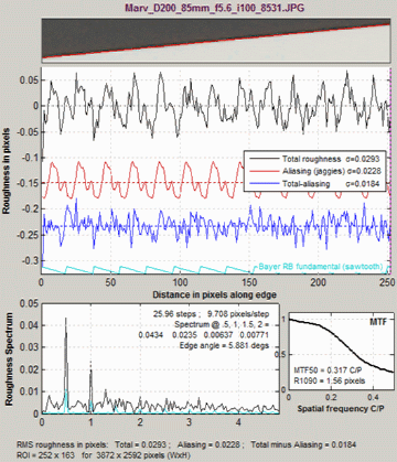 Edge roughness plot Edge roughness plot |
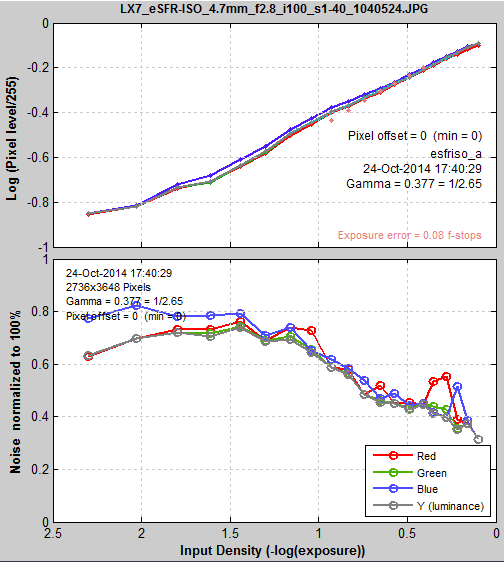
Noise ploteSFR ISO can display several types of noise, measured from the grayscale patches surrounding the center of the chart, including all types of noise calculated by Color/Tone Interactive and Color/Tone Auto (standard pixel noise, chroma noise, scene-referenced noise, sensor (raw) noise, and ISO-15739 visual noise). SNR (Signal-to-Noise Ratio) can also be displayed as a ratio or in dB. Instructions for selecting the noise display and x-axis and descriptions of the noise displays are on Color/Tone Interactive/Color/Tone Auto and eSFR ISO Noise.
The figure on the right— simple pixel noise, expressed as a percentage of the maximum pixel value— is one of the simpler noise displays.
Noise plot (for simple pixel noise) |
 |
Wedge plotIf the Enhanced or Extended chart has been photographed and the Wedge checkbox in the eSFR ISO Setup window has been checked, the four wedge pairs are automatically detected, and one of two results for each pair (MTF and Aliasing onset, shown on the right, and Moiré) can be displayed. These plots are described in detail in the Wedge module page.
Wedge MTF and Aliasing onset plot |
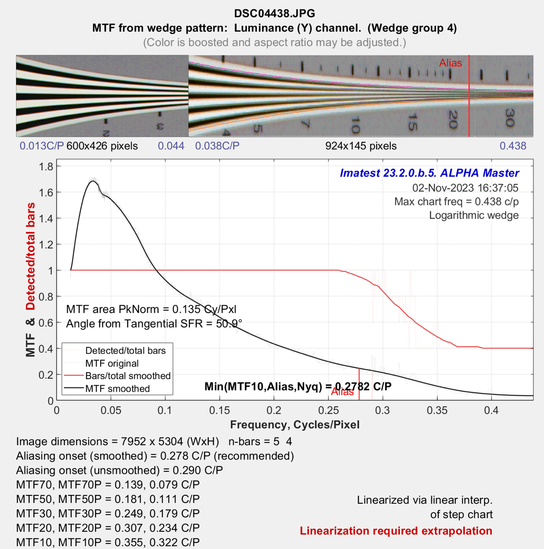 |
Multi-Wedge plot
The Multi-Wedge plot shows a summary of results for all wedges. It is the exact counterpart of the Multi-ROI (edge) summary plot, illustrated above.
|
The multi-ROI (multiple Region of Interest) summary, shown in the Rescharts window (above), contains a summary of eSFR ISO wedge results. The upper left contains the image in muted gray tones, with the selected high frequency wedge regions surrounded by red rectangles and displayed with full contrast. The low frequency wedge regions, which are primarily for low frequency normalization, are inside blue rectangles. Up to four results boxes are displayed next to each region. The results can be selected in the the Display options area on the right, below the Display selection. There is a legend below the image. |
Alias onset, MTF50, MTF20 Results selection |
View selection |
Notes:
- The onset of aliasing is the frequency where the number of detected bars (smoothed to reduce sensitivity to noise) drops to 95% of the low frequency value. It is only indicative of aliasing on relatively sharp systems (good lenses in good focus, so there is some energy around the Nyquist frequency).
-
min(MTF10, alias, Nyq) (the minimum of MTF10, the onset of aliasing, and the Nyquist frequency (0.5C/P)) is the proposed ISO 16505 resolution metric (selected because MTF10 is not robust). See “Measuring MTF with wedges: Pitfalls and best practices” (presented at the Electronic Imaging 2017 conference).
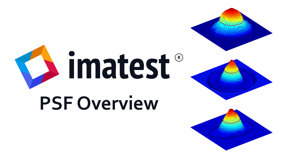
PSF Plot
Imatest can estimate an imaging system’s loss of resolution (PSF) using a pair of collocated, near-sagittal and tangential slanted edges on SFRplus, eSFR ISO and SFRreg targets. Easily analyze and improve sharpness, chromatic aberration, and distortion measurements.
eSFR ISO summary
- eSFR ISO analyzes images of the ISO 12233:2014 Edge MTF chart. There should be few or no interfering patterns (bars, etc.) outside the image of the chart itself.
- Lighting should be even and glare-free. Lighting and alignment recommendations are given in Building a test lab.
- The first time eSFR ISO is run, it should be run through Rescharts. This allows
- parameters to be adjusted and saved for later use in the automatic version of eSFR ISO, which is opened with the button in the Imatest main window.
- results (listed above) to be examined interactively in the Rescharts window.
- Subsequent runs can be done with eSFR ISO Auto, which is not interactive, but allows batches of image files to be analyzed.
Result file names— The roots of the file names are the same as the image file name. The channel (Y, R, G, or B) is included in the file name. If a Region of Interest has been selected from a complete digital camera image, information about the location of the ROI is included in the file name following the channel. For example, if the center of the ROI is above-right of the image, 20% of the distance from the center to the corner, the characters AR20 are included in the file name.
(default location: subfolder Results)
| Excel .CSV (ASCII text files that can be opened in Excel) | |
| SFR_cypx.csv | (Database file for appending results: name does not change). Displays 10-90% rise in pixels and MTF in cycles/pixel (C/P). |
| SFR_lwph.csv | (Database file for appending results: name does not change). Displays 10-90% rise in number/Picture Height (/PH) and MTF in Line Widths per Picture Height (LW/PH). |
| filename_YA17_MTF.csv or | Excel .CSV file of MTF results for this region (designated by location (YA17) or sequence (nn = 01,...). All channels (R, G, B, and Y (luminance) ) are displayed. |
| filename_Y_multi.csv | Excel .CSV file of summary results for a multiple ROI run. |
| filename_Y_sfrbatch.csv | Excel .CSF file combining the results of batch runs (one or more files) with multiple ROIs. Only for automatic eSFR ISO (not Rescharts). Used as input to Batchview. |
Excel .CSV (Comma-Separated Variables) and XML output
Imatest SFR creates or updates output files for use with Microsoft Excel. The files are in CSV (Comma-Separated Variable) format, and are written to the Results subfolder by default. .CSV files are ASCII text files that look pretty ugly when viewed in a text editor:
|
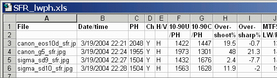
File ,Date/time ,PH,Ch,H/V,10-90U,10-90C,Over-,Over-,MTF50U,MTF50C,MTF,Camera,Lens,FL,f-stop,Loc,Misc.,,,,,/PH,/PH,shoot%,sharp%,LW/PH,LW/PH,Nyq,,,(mm),,,settings canon_eos10d_sfr.jpg,2004-03-19 22:21:34, 2048,Y,H, 1422, 1447, 19.5, -0.7, 1334, 1340,0.154,,,,, canon_g5_sfr.jpg,2004-03-19 22:24:30, 1955,Y,H, 1973, 1301, 48.0, 21.3, 1488, 1359,0.268,Canon G5,—,14,5.6,ctr, sigma_sd9_sfr.jpg,2004-03-19 22:27:55, 1504,Y,H, 1432, 1676, 2.4, -7.7, 1479, 1479,0.494,,,,, sigma_sd10_sfr.jpg,2004-03-19 22:28:32, 1504,Y,H, 1563, 1628, 11.9, -2.0, 1586, 1587,0.554,,,,, |
But they look fine when opened in Excel.
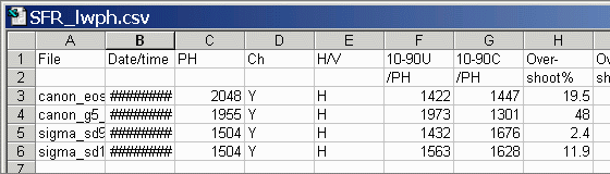
.CSV files can be edited with standard text editors, but it makes more sense to edit them in Excel, where columns as well as rows can be selected, moved, and/or deleted. Some fields are truncated in the above display, and Date/time is displayed as a sequence of pound signs (#####...).
The format can be changed by dragging the boundaries between cells on the header row (A, B, C, ...) and by selecting the first two rows and setting the text to Bold. This makes the output look better. The modified file can be saved with formatting as an Excel Worksheet (XLS) file. This, of course, is just the beginning.
It's easy to customize the Excel spreadsheet to your liking. For example, suppose you want to make a concise chart. You can delete Date/time (Row B; useful when you're testing but not so interesting later) and Channel (all Y = luminance). You can add a blank line under the title, then you can select the data (rows A4 through J7 in the image below) and sort on any value you choose. Corrected MTF50 (column I) has been sorted in descending order. Modified worksheets should be saved in XLS format, which maintains formatting.
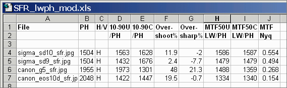
There are no limits. With moderate skill you can plot columns of results. I've said enough. ( I'm not an Excel expert! )
Summary .CSV and XML
files for MTF and other data
An optional .CSV (comma-separated variable) output file contains results for MTF and other data. Its name is [root name]_[channel location]_MTF.csv, where channel is (R, G, B, or Y) and the location BL75 means below-left, 75% of the distance to the corner (from the center). An example is Canon_17-40_24_f4_C1_1408_YBL75_MTF.csv. Excerpts are shown below, opened in Excel.
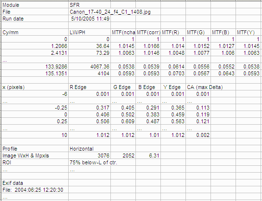
A portion of the summary CSV file, opened in Excel
The format is as follows:
| Line 1 | Imatest, release (1.n.x), version (Light, Pro, Eval), module (SFR, SFR multi-ROI, Colorcheck, Stepchart, etc.). |
| File | File name (title). |
| Run date | mm/dd/yyyy hh:mm of run. |
| (blank line) | |
| Tables | Separated by blank lines if more than one. Two tables are produced. |
| The first table contains MTF. The columns are Spatial frequency in Cy/mm, LW/PH, MTF (selected channel), MTF (Red), MTF (Green), MTF (Blue), MTF (Luminance = Y). (...) represent rows omitted for brevity. | |
| The second table contains the edge. Columns are x (location in pixels), Red edge, Green edge, Blue edge, Luminance (Y) edge, and Chromatic Aberration (the difference between the maximum and minimum). | |
| (blank line) | |
| Additional data | The first entry is the name of the data; the second (and additional) entries contain the value. Names are generally self-explanatory (similar to the figures). |
| (blank line) | |
| EXIF data | Displayed if available. EXIF data is image file metadata that contains important camera, lens, and exposure settings. By default, Imatest uses a small program, jhead.exe, which works only with JPEG files, to read EXIF data. To read detailed EXIF data from all image file formats, we recommend downloading, installing, and selecting Phil Harvey's ExifTool, as described here. |
This format is similar for all modules. Data is largely self-explanatory. Enhancements to .CSV files will be listed in the Change Log.
The optional XML output file contains results similar to the .CSV file. Its contents are largely self-explanatory. It is stored in [root name].xml. XML output will be used for extensions to Imatest, such as databases, to be written by Imatest and third parties. Contact us if you have questions or suggestions.
An optional .CSV file is also produced for multiple ROI runs. Its name is [root name]_multi.csv.
Links
How to Read MTF Curves by H. H. Nasse of Carl Zeiss. Excellent, thorough introduction. 33 pages long; requires patience. Has a lot of detail on the MTF curves similar to the Lens-style MTF curve in SFRplus and eSFR ISO. Even more detail in Part II. Their (optical) MTF Tester K8 is of some interest.
Understanding MTF from Luminous Landscape.com has a much shorter introduction.
Understanding image sharpness and MTF A multi-part series by the author of Imatest, mostly written prior to Imatest's founding. Moderately technical.
Bob Atkins has an excellent introduction to MTF and SQF. SQF (subjective quality factor) is a measure of perceived print sharpness that incorporates the contrast sensitivity function (CSF) of the human eye. It will be added to Imatest Master in late October 2006.
Optikos makes instruments for measuring lens MTF. Their site has some interesting articles, for example, Lens Testing: The Measurement of MTF (Modulation Transfer Function).