A key result of the SFR, SFRplus, and eSFR ISO modules
If you entered Imatest on this page, you may want to explore the background information in these links.
Sharpness introduces sharpness measurements and MTF.
How to test Lenses with Imatest contains concise instructions on testing lenses
using SFRplus and eSFR ISO.
Image quality factors lists the factors measured by Imatest.
Table of contents (documentation)
Imatest SFR, SFRplus and eSFR ISO display Edge profiles and SFR (Spatial frequency response, i.e., MTF) plots with spatial frequency labeled in one of the following units:
- Cycles per Pixel (C/P)
- Cycles per distance (mm or inches )
- Line Widths or Pairs per Picture Height (LW/PH or LP/PH)
- Cycles per angle (milliradians or degrees)
- Cycles per object distance (mm or inches)
depending on settings of the Plot section of the SFR settings box , shown below. Note that one cycle (or line pair) is equivalent to two line widths.
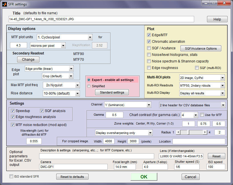 SFR settings window
| Key results are shown below in Bold. The most important is MTF50, the spatial frequency where contrast drops to half (50%) of its low frequency value. MTF curves and Image appearance contains several examples illustrating the correlation between MTF curves and perceived sharpness.
MTF50P (the spatial frequency where contrast drops to half (50%) of its peak value) is also extremely important because it is less inflated by extreme sharpening, which causes “halos” near edges in the image. It is identical to MTF50 for low to moderate sharpening (where the MTF peak is less than 1).
Standardized sharpening results are no longer displayed on this page because they are generally not recommended for lens and system testing (Standardized sharpening was designed for comparing cameras with differing degrees of software sharpening, where RAW files were unavailable.) See Sharpening and Standardized Sharpness for details.
|
|
Edge response (Spatial domain plot– upper-left)
| Black line |
Edge profile for the luminance (Y) channel, where Y = 0.21*R, 0.72*G, 0.07*B. The normalized edge profile is proportional to the light intensity. You may also select to display |
 Edge profile Edge profile |
| |
- Line Spread Function (LSF; the derivative of the edge profile), shown below,
- Pixel levels (which includes gamma-encoding), or
- Edge linear unnormalized to view the unnormalized edges, which often gives a better idea of the degree of saturation that can affect results.
|
R, G, and B
dashed lines
|
Edge profile for the R, G, and B channels (Imatest Master-only). Shown more prominently in the Chromatic Aberration plot. |
|
Pale brown
dashed line
|
Edge profile for a diffraction-limited lens at this aperture (obtained from EXIF data). Pixel spacing and Wavelength (um) for diffraction-ltd MTF must be entered. |
|
Left column
text
(input settings)
|
| Plot description, including measurement orientation. (A vertical edge is used for a horizontal profile.) |
| Image height (H) or Width x Height (WxH) in pixels |
| Total megapixels |
Channel. Defaults to Y (luminance). R, G, or B are also available. YR60 is a designation for Y-channel, Right of center, 60% of the distance from the center to the corner.
|
| Gamma is an estimate of camera gamma used to linearize the image. Defaults to 0.5. |
Edge angle in degrees
|
|
Right column
text
(results) |
| 10-90% rise distance (original; uncorrected) in pixels and rises per picture height (PH). |
| [Imatest Master only] 10-90% rise distances of the R, G, and B channels, individually. Imatest Master only. |
| Overshoot and undershoot. Percentage of step amplitude. Shown if appropriate. |
| Average pixel levels in dark and light areas, and light/dark ratio. Clipping can occur if they are too close to 0 or 255. Also gives the ratio between the light and dark areas: an indication of the contrast of the image. |
|
Line Spread Function (Spatial domain plot– upper left)
|
The line spread function (LSF; the derivative of the edge spread function) can selected for display instead of the Edge profile if it’s selected in the Edge plot box in the SFR/SFRplus settings window.
The following results appear on the right of the plot when LSF is selected.
- Peak LSF (maximum d(Edge)/dx) in pixels
- PW50 (50% pulse width; also called Full Width at Half-Maximum FWHM) in pixels and pulse widths per picture height (PH).
- RMS edge roughness in pixels. A promising measurement related to image quality. Shown on the right.
|
 Line Spread Function (LSF) Line Spread Function (LSF) |
Spatial Frequency Response (MTF) (lower-left)
| Black line (bold) |
Spatial Frequency Response (MTF) for the luminance (Y) channel. MTF curves and Image appearance contains several examples illustrating the correlation between MTF curves and perceived sharpness. |
 MTF plot MTF plot |
R, G, and B
dashed lines |
Spatial Frequency Response for the Red, Green, and Blue channels (Imatest Master-only). |
Pale brown
dashed line |
MTF for a diffraction-limited lens at this aperture (obtained from EXIF data). Pixel spacing must be entered. |
Right column
text (results) |
| MTF50 (50% contrast spatial frequency) for the image in cycles/pixel and line widths per picture height (LW/PH). Its relationship to print quality is discussed in Interpretation of MTF50. |
| MTF50P (spatial frequency where contrast is 50% of its peak value) for the original uncorrected image in cycles/pixel and line widths per picture height (LW/PH). This is the same as MTF50 for slightly to moderately sharpened edges, but smaller for oversharpened edges. It may be a better indicator than MTF50 of the perceived sharpness of oversharpened images. |
| Oversharpening or undersharpening. The amount the camera is over- or undersharpened with respect to standardized sharpening. 100% ( MTF( feql ) – 1) where feql is the frequency where MTF is set to 1 by standardized sharpening. |
| Secondary Readout Up to two secondary readouts can be selected in the SFR settings window. You can select MTFxx, the spatial frequency for xx% contrast, MTFxxP, the spatial frequency where MTF is xx% of its peak value, the MTF at a specified spatial frequency, or MTF normalized to its peak value (a very interesting result that closely tracks MTF50 for low to moderately sharpened images, but does not increase as extreme sharpening is applied).
MTF20P (spatial frequency where contrast is 20% of peak value) and MTF area normalized to 1 at the peak value.
MTF Area PkNorm (MTF normalized to its peak value). Valuable because it does not reward extreme sharpening; it is nearly identical to MTF50 up to the onset of oversharpening, then it remains relatively constant as the sharpening peak increases above 1.
|
| MTF at the Nyquist frequency. May indicate of the effectiveness of the anti-aliasing filter and likelihood of aliasing effects such as Moire patterns. But it not an unambiguous indicator because aliasing is related to sensor response, and MTF at Nyquist is the product of sensor response, the demosaicing algorithm, and sharpening, which can boost response at Nyquist. Aliasing effects may become serious over 0.3. There is a tradeoff: the more effective the sensor anti-aliasing, the poorer the sharpness. (See the Imaging-Resource.com review of the Nikon D800E for an interesting discussion.) Foveon sensors (three colors per pixel) are more tolerant of aliasing than Bayer sensors, which are used in most digital cameras. |
| Nyquist frequency: Half the sampling rate = 1/(2*pixel spacing). Always 0.5 cycles/pixel. Indicated by the vertical blue line. |
|
Image and EXIF data (on right)
| Right: Input data |
 |
| |
Top right image
Thumbnail of the entire image, showing the location of the selected Region of Interest (ROI) in red. |
| |
Middle right image
The selected Region of Interest (ROI), shown with the correct aspect ratio, but not necessarily the exact size. The following parameters are displayed below the image.
- ROI size in pixels
- ROI boundary locations (Left, Right, Top, and Bottom) in pixels from the upper-left corner,
- Edge angle in degrees, and
- Estimated chart contrast, derived from the average pixel levels of the light and dark areas (away from the transition) and gamma. The equation: Estimated chart contrast = (avg. pixel level of light area/avg. pixel level of dark area)^(1/gamma)
|
| |
Lower right text
Selected EXIF data: metadata recorded by the digital camera. Only for JPEG files unless Phil Harvey’s ExifTool (recommended) is installed. May include ISO speed, aperture, and other details. Thanks to Matthias Wandel for jhead.exe.
|

