Note: This page is not quite complete, but we felt that the results are
important enough to be presented in its present (nearly complete) state.
Method – Results – MTF50 failure – MTF Area
Related page: Correcting Misleading Image Quality Measurements:
links to an Electronic Imaging paper that compares MTF summary metrics
In this page we analyze the consistency of slanted-edge MTF measurements, focusing on the effects of noise and region size on measurement consistency. We describe the test procedure in sufficient detail to enable Imatest users to perform similar studies for themselves.
We also discuss some important and recognizable situations where consistency may be compromised. these include
- systems with strong response above the Nyquist frequency (0.5 cycles/pixel), which can result in low frequency artifacts that affect consistency, and
- systems with inappropriate sharpening that shape the MTF response curve so that summary metrics like MTF30 and MTF50 become unstable
We propose a new summary metric: the area under the MTF curve (up to the Nyquist frequency), normalized to the peak MTF value. This metric is relatively unfamiliar, but seems to be generally more stable than MTF50 and MTF50P.
Method
The tests were performed on the Panasonic Lumix LX100 camera: a high quality compact camera that has a relatively large sensor, excellent controls, and can produce both JPEG and raw files. We took 10 images of a large eSFR ISO test chart at each of three ISO speeds, saving them in both JPEG and raw formats, for a total of 60 images. (SFRplus could have been used with equally good results.) The lens was set to 50mm-equivalent focal length. Manual focus was used to eliminate variations due to autofocus. Standard signal processing was selected. A 2-second time delay minimized camera shake.
| ISO Speed | Comments |
| 200 | Base ISO speed of the LX100. Lowest noise. |
| 1600 | High ISO speed for good image quality in fairly dim light. Moderate noise. |
| 12800 | Extreme ISO speed for very dim light. High noise. |
The sequence of operations is
- Run eSFR ISO in Rescharts (eSFR ISO setup) mode to make and save settings and to verify the calculations. This is required to prepare for the batch eSFR ISO runs used for the actual consistency calculations.
- Run each batch of ten files using eSFR ISO Auto. Check to be sure that files named [root file name]_sfrbatch.csv, where key results are stored, have been created.
- If extremely small regions need to be analyzed (smaller than what you get with the 0.4 ROI size setting), the same batch of files can be run in SFR (with manual region selection). Use different framing for JPEG and raw image because they are framed differently: the JPEG is slightly cropped to correct for optical distortion.
- Run Batchview (shown below) using the [root file name]_sfrbatch.csv output files from the batch eSFR ISO runs to get a statistical analysis (means and standard deviations) of key results from the batch of runs (MTF50, MTF50P, etc.). This analysis is meaningful for sequences of identical images.
|
An Edge ID file with one ROI in each of the center, part-way, and corner zones of the image was used in eSFR ISO so that Batchview, which analyzes the mean of results for each zone, analyzes just one image per zone. (Otherwise you would get the mean of several measurements, which would have a lower variability). The edge ID shown on the right (format: x_y_LRTB) was chosen because the sharpest edge in the manually-focused image was the left edge of the slanted-square two squares to the right of the center. This square (region 3 in the figure below) was used for the analyses on this page. |
Edge ID 0_0_R |
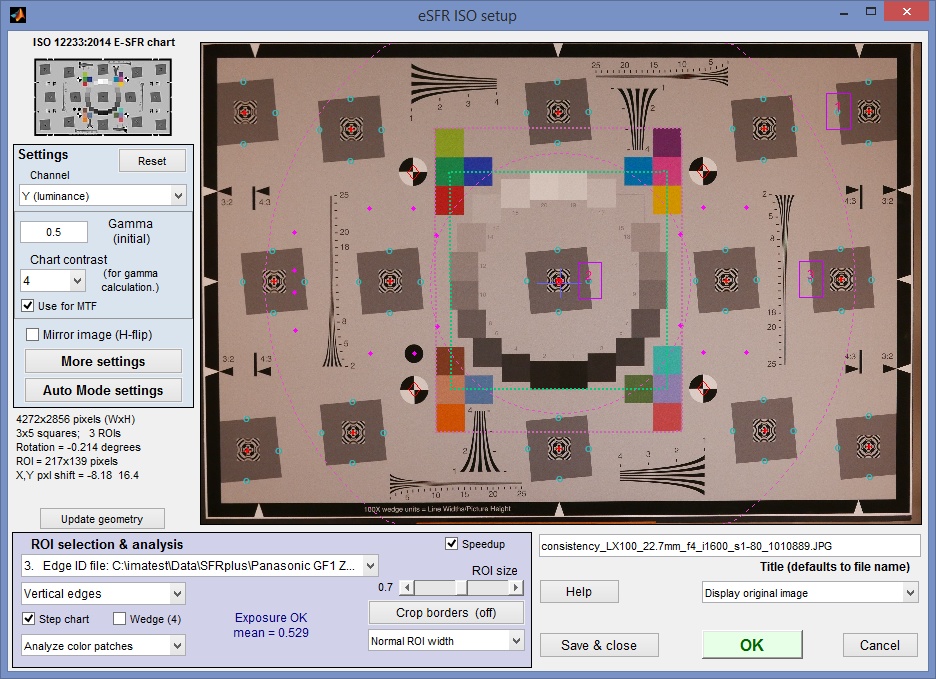 eSFR ISO setup window
Other settings:
In the eSFR ISO More settings window, MTF plot units were set to LW/PH, Speedup was checked, and MTF noise reduction (mod apod) was checked (except where indicated).
In the eSFR ISO Auto mode settings window, all Single-region plots and most Multi-ROI plots were unchecked. (When we needed to examine details we ran eSFR ISO Setup). Close figures after save and Allow CSV file output were checked.
In running eSFR Auto, select batches of files to be analyzed together, i.e., don’t mix different ISO speeds or JPEG and raw, unless there is a specific need to do so (for example, for directly comparing different ISO speeds). No additional settings need to be entered, since they were saved during eSFR Setup (Rescharts).
In Batchview, enter the […]_sfrbatch.csv output files (from the eSFR ISO batch runs) into boxes A–D at the bottom. Up to four output files can be entered for comparison (though statistical results can only be viewed when a single batch is displayed: Display (lower-right) should be set to A, B, C, or D. The measurement (MTF50, MTF50P, etc.) should be selected from the dropdown menu at the top-left. For this particular analysis, Part way mean was selected in the Region dropdown menu, top-center. (Center mean will be selected in cases where the image is sharpest in the center.) Statistics (mean, sigma) should be selected in the dropdown menu on the top-right (only visible with a single batch is displayed).
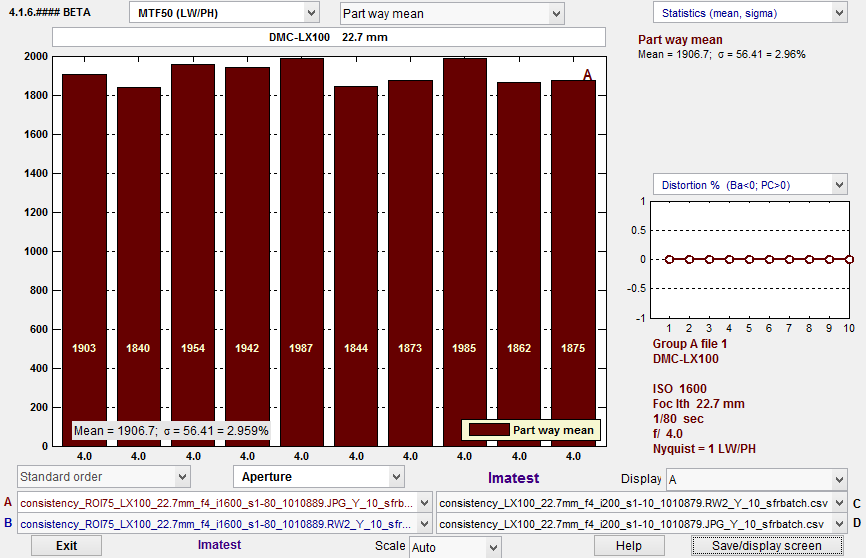 Batchview results for 10 eSFR ISO images: JPEG @ ISO 1600 (Display A)
Results
| Abbreviation | Full name | Description |
| S/N (linearized) |
Signal-to-Noise ratio (SNR), from the linearized image | Signal-to-Noise ratio (SNR), for the Dark and light areas of the Region of Interest (ROI) of the linearized image (after gamma has been removed) used to calculate MTF. Taken at a sufficient distance from the transition so illumination should be relative flat. This is a simple ratio. To get decibels (dB), take 20 log10 of this number. |
| MTF50* | MTF50 | Spatial frequency where contrast is 50% of the low frequency level. The most widely-used sharpness summary metric. Corresponds to lowpass filter bandwidth in Electrical Engineering. Continues to increase as sharpening is increased, even if the sharpening “halo” badly damages image quality. |
| MTF50P* | MTF50P | Spatial frequency where contrast is 50% of the peak level. Corresponds to bandpass filter bandwidth. Identical to MTF50 for low to moderate sharpening, but increases more slowly for strong oversharpening. |
| MTF20* | MTF20 | Spatial frequency where contrast is 20% of low frequency level. Close to the vanishing resolution (which may be closer to MTF10, but MTF10 is often strongly affected by noise). |
| R1090 /PH | 10-90% Rise Distance per PH | The 10-90% rise distance expressed in rises per Picture Height. Strongly correlated with 1/MTF50. May fail if there is a ramp in the edge response caused by flare light. |
|
MTF Area* MTFAPN |
MTF Area (Peak Normalized) | The integral of the MTF from 0 to the Nyquist frequency ( fNyq = 0.5 Cycles/Pixel), where MTF is normalized to a peak value of 1. Can be displayed as a Secondary readout in any Imatest MTF module. Closely approximates MTF50 for low to moderate sharpening, but flattens out for high sharpening (where the sharpening peak > 1). May be the most stable sharpness summary metric because it is the integral over a range of frequencies instead of the property of a single frequency, and because it is relatively insensitive to oversharpening, i.e., it does not reward extreme oversharpening. See Appendix (below) for more details. |
| *These measurements are summary metrics derived from the MTF curve. | ||
| ISO Speed and image format |
Signal/Noise (linearized) Dark / Light |
Mean / Standard deviation (%) (MTF in LW/PH = Line Widths/Picture Height) | ||||
| MTF50 | MTF50P | MTF20 | R1090 /PH | MTF Area |
||
| RAW ISO 200 | 34 / 50.6 | 1262 / 3.82% | 1262 / 3.82% | 2470 / 4.66% | 1084 / 2.77% | 1425 / 1.46% |
| JPEG ISO 200 | 37.3 / 84 | 1961 / 1.77% | 1961 / 1.77% | 2528 / 2.11% | 1872 / 2.01% | 1931 / 1.78% |
| RAW ISO 1600 | 13.3 / 18.6 | 1259 / 7.41% | 1258 / 7.41% | 2392 / 11.3% | 1072 / 4.62% | 1404 / 2.71% |
| JPEG ISO 1600 | 16.1 / 31.5 | 1907 / 2.96% | 1907 . 2.96% | 2460 / 3.41% | 1816 / 3.65% | 1857 / 2.53% |
| RAW ISO 12800 | 6.56 / 9.28 | 1129 / 18.8% | 1126 / 18.5% | 2173 / 19.2% | 1033 / 7.39% | 1440 / 5.53% |
| JPEG ISO 12800 | 15.6 / 35.1 | 1624 / 6.4% | 1624 / 6.4% | 2270 / 3.44% | 1494 / 6.09% | 1558 / 3.6% |
| ISO Speed and image format |
Mean / Standard deviation (%) (MTF in LW/PH = Line Widths/Picture Height) | ||||
| MTF50 | MTF50P | MTF20 | R1090 /PH | MTF Area |
|
| RAW ISO 200 | 1270 / 4.48% | 1270 / 4.48% | 2502 / 4.92% | 1123 / 2.11% | 1438 / 1.4% |
| JPEG ISO 200 | 1981 / 2.1% | 1981 / 2.1% | 2559 / 2.64% | 1906 / 2.38% | 1952 / 2.15% |
| RAW ISO 1600 | 1259 / 9.26% | 1259 / 9.26% | 2281.8 / 11.9% | 1118 / 4.42% | 1412 / 4.19% |
| JPEG ISO 1600 | 1910 / 3.38% | 1910 / 3.38% | 2477 / 4.14% | 1811 / 2.71% | 1897 / 2.95% |
| RAW ISO 12800 | 1160 / 16.4% | 1157 / 16.7% | 2180 / 22.5% | 1095 / 11.7% | 1470 / 7.0% |
| JPEG ISO 12800 | 1666 / 8.1% | 1666 / 8.1% | 2282 / 4.97% | 1512 / 7.91% | 1584 / 5.3% |
| ISO Speed and image format |
Mean / Standard deviation (%) (MTF in LW/PH = Line Widths/Picture Height) | ||||
| MTF50 | MTF50P | MTF20 | R1090 /PH | MTF Area |
|
| RAW ISO 200 | 1296 / 3.81% | 1296 / 3.81% | 2496 / 4.5% | 1150 / 3.59% | 1433 / 1.19% |
| JPEG ISO 200 | 2014 / 2.09% | 2014 / 2.09% | 2584 / 2.68% | 1934 / 2.17% | 1972 / 1.75% |
| RAW ISO 1600 | 1371 / 11.1% | 1371 / 11% | 2435 / 14% | 1124 / 7.71% | 1430 / 3.93% |
| JPEG ISO 1600 | 1966 / 4.2% | 1962 / 4.32% | 2751 / 22.7%* | 1867 / 2.36% | 1910 / 3.16% |
| RAW ISO 12800 | 1347 / 21% | 1340 / 20.9% | 2611 / 32.9% | 1230 / 14.9% | 1489 / 10.1% |
| JPEG ISO 12800 | 1662 / 8.6% | 1662 / 8.6% | 2294 / 6.77% | 1528 / 11.6% | 1609 / 6.2% |
*MTF20 had a serious outlier. The mean would have been around 2550 without it.
| ISO Speed and image format |
Mean / Standard deviation (%) (MTF in LW/PH = Line Widths/Picture Height) | ||||
| MTF50 | MTF50P | MTF20 | R1090 /PH | MTF Area |
|
| RAW ISO 200 | 1314 / 3.14% | 1314 / 3.14% | 2477 / 3.94% | 1178 / 3.55% | 1483 / 1.57% |
| JPEG ISO 200 | 2027 / 2.43% | 2027 / 2.43% | 2680 / 3.51% | 1933 / 2.34% | 2030 / 2.04% |
| RAW ISO 1600 | 1339 / 12.1% | 1339 / 12.1% | 2698 / 23.8% | 1195 / 14.1% | 1509 / 6.56% |
| JPEG ISO 1600 | 2001 / 6.62% | 1993 / 6.61% | 2893 / 34.5%* | 1901 / 4.02% | 1978 / 6.03% |
| RAW ISO 12800 | 1311 / 25.6%* | 1298 / 25.7%* | 1818 / 45.5%* | 1229 / 22.3%* | 1562 / 12.5% |
| JPEG ISO 12800 | 1639 / 9.9% | 1639 / 9.9% | 2269 / 8.39% | 1593 / 12.2% | 1620 / 7.86% |
Notes:
- MTF50P is generally identical to MTF50 because the images tested were not oversharpened (the maximum MTF level was 1.0.).
- Standard deviations (σ) greater than 10% indicate the the measurement has serious variability. Recall that the measurement spread (maximum – minimum) is generally considerably larger than σ. Measurements with σ > 20% (for example, several of the measurements of the RAW image, 50×80 pixel ROI, ISO 12800) are completely unreliable, i.e., useless.
- Signal/Noise (SNR) is roughly proportional to 1/(ISO Speed)1/2 in raw images, i.e., SNR drops by half when ISO speed is quadrupled. The relationship is less clear with JPEG images because of signal processing changes with ISO speed (there is typically more noise reduction at higher ISO speeds).
Conclusions
MTF Area is a superior summary metric for sharpness: it is much more stable than MTF50. It is relatively unfamiliar.
A 25×40 pixel region size is sufficient for good results with low noise images. This may be the best that can be done with low resolution cameras, though larger is recommended if the geometry allows or if the image is very noisy.
An image where MTF50 fails
|
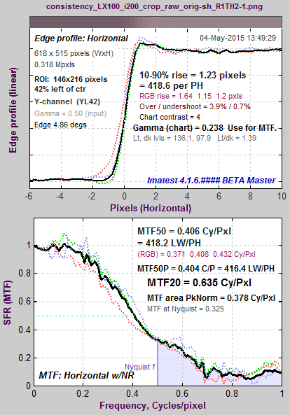
A customer sent us an image whose MTF50 measurements varied unpredictably as ROI size changed. A crop is shown on the right. You can click on it to view a full-sized image that you can download and run. Running the image (using SFRplus with the original uncropped image; SFR with the crop) quickly showed the reason for the problem. A curious combination of excellent lens performance and large sharpening radius (appropriate for a mediocre lens) resulted in a long ramp in the MTF response around the 50% level. Slight changes in response could have major changes in MTF50. This problem will not occur if MTF Area (a relatively unfamiliar summary metric, described below) is used instead of MTF50. |
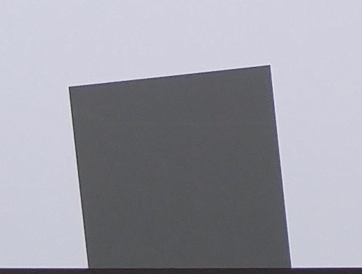 Click on the image to view a full-sized image that can be downloaded. |
|
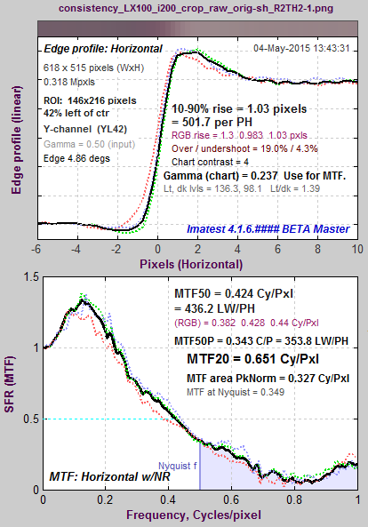
As explained in the Sharpening page, the sharpening transfer function is periodic with a period of 1/Radius in Cycles/Pixel. The system MTF (shown on the right for the above image) is the the raw MTF response times the sharpening transfer function. 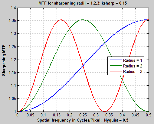 Sharpening transfer function as a function The pattern of peaks and dips (near 0.42 and 0.84 C/P) suggests a sharpening radius of around 2.4, which would have its first peak around 0.24 C/P. The first system MTF peak is typically lower because of the MTF rolloff of the unsharpened image. |
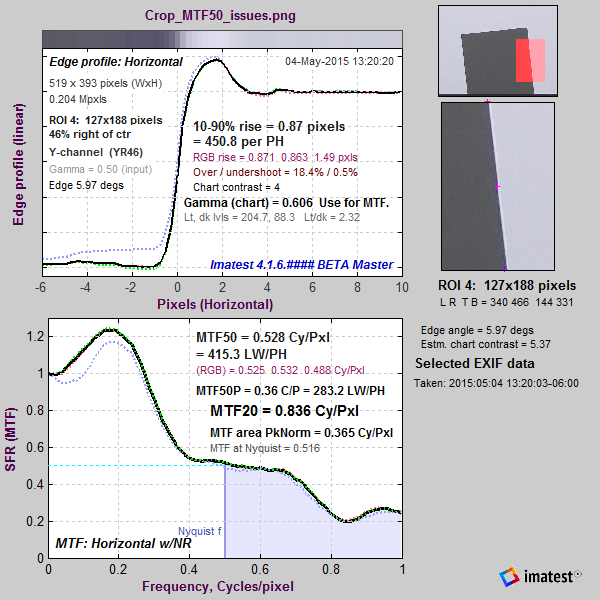 Average edge and MTF Average edge and MTF |
 The strong response above the Nyquist frequency (0.5 cycles/Pixel) indicates that the lens is extremely sharp. Images from such lenses tends to look best with sharpening radii well below 2.4, which provides very little response boost in the important 0.35-0.5 C/P range, where the input MTF has sufficient energy to benefit from the boost.
This image may look good on the small display of a camera phone, but it is far from optimum when exported and viewed on a large display or printed. When sharpened in this way, image quality won’t approach the potential of the lens and sensor. A better strategy would have been to sharpen with a radius between 1 and 1.5 (perhaps with a moderate oversharpening peak— see sharpening examples, below), then to add additional sharpening for images sent to the display.
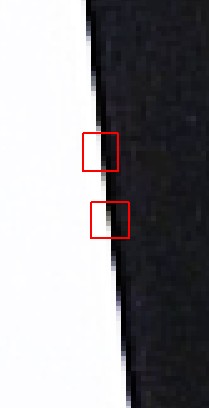
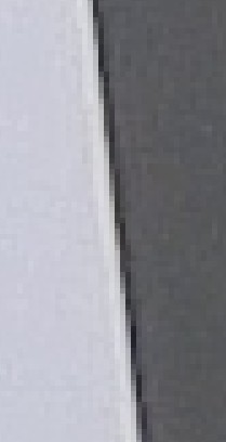
When the system has strong response above the Nyquist frequency, low frequency artifacts such as Moiré fringing or stair-stepping may appear. Stair-stepping is clearly visible when the above image is magnified 5X, as shown on the right. These artifacts have an adverse effect on measurement consistency because an important step in the slanted-edge measurement is the estimate of the edge angle, which is quite consistent for smoothed (anti-aliased) edges, but which depends on the ROI position when there is extreme aliasing. A highly exaggerated example is shown on the far right, where the edge angle estimate derived from the two small red rectangles will be completely different.
Appendix: MTF50 vs. MTF Area Peak-Normalized
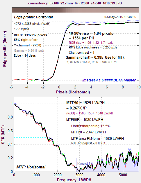
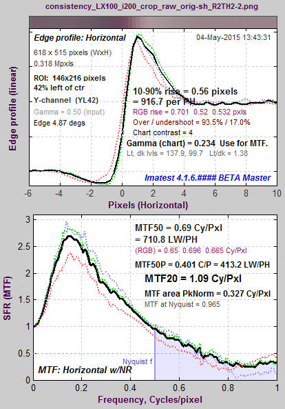
The plot below shows the edge and MTF from a raw image captured at ISO 12800. It is extremely noisy because of the very high ISO speed (dim illumination of the sensor, followed by very high gain) and because no noise reduction is applied to raw images.
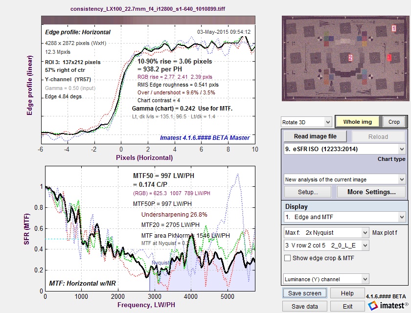 MTF curve for raw file taken at ISO 12800
|
A key observation (not obvious with normal images, which have much less noise) is that MTF50 is based on the first spatial frequency where MTF drops below 50% of the low frequency level— 997 LW/PH in this plot, where noise causes a sudden and misleading dip just under 1000 LW/PH in the (unsmoothed) MTF curve. Smoothing the MTF plot would improve MTF measurement consistency, but smoothing has never been addressed in the ISO 12233 standard. The optimum amount of smoothing, which depends on the width of the region (i.e., frequency increment or the number of points in the plot) would have to be determined. A second observation is that MTF Area (short for MTF Area Peak-Normalized), which is equal to the integral of the MTF curve from 0 the Nyquist frequency fNyq, would be closely approximate MTF50 derived from a properly-smoothed monotonically-decreasing MTF curve. Another advantage of MTF Area is that it tracks MTF50, i.e., it increases as sharpening increases, up to the point where an overshoot appears in the sharpened MTF curve (peak MTF > 1), then it remains relatively constant. So it does not reward excessive sharpening with better numbers. |
 MTF for JPEG @ ISO 12800. Same image capture, same region as above. Lower noise; some sharpening visible. |
|
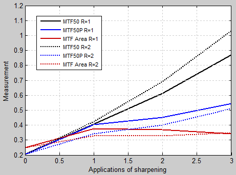
This is illustrated in the plot on the right, which shows MTF50, MTF50P and MTF Area for an edge (from one of the ISO 200 raw images in the above analysis). The edge was analyzed without sharpening, and with one and two applications of sharpening (Unsharp Mask in Picture Window Pro with Sharpening Radii = 1 and 2). MTF50 continues to increase as sharpening increases, even though the visible effect of sharpening— “halos” near edges— can degrade image appearance. MTF50P increases much more slowly: it’s a generally more reliable metric than MTF50. But it still depends on a single frequency. MTF area does not increase once a sharpening peak > 1 appears. Now that these statistical results are available, Imatest will be doing more to promote the use of MTFAPN as a sharpness summary metric. |
 |
 A. No sharpening A. No sharpening |
 B. 1 sharpen, R = 1 B. 1 sharpen, R = 1 |
 C. 2 sharpens, R = 1 C. 2 sharpens, R = 1 |
 D. 1 sharpen, R = 2 D. 1 sharpen, R = 2 |
 E. 2 sharpens, R = 2 E. 2 sharpens, R = 2 |
There may be cases where moderate MTF overshoot (~25-50%) may be desirable. In such cases a modified version of MTF Area may be a better metric. For example (for sharpening between B. and C, above), an image with a spatial domain overshoot of 25% may appear sharper than it would without overshoot— and the halo won’t be very visible. This corresponds to a peak MTF of approximately 1.4. For a desired peak MTF = MTFpk > 1, we define
\( MTF_{Area} (MTF_{pk}) = \text{min}(\text{measured MTF peak, }MTF_{pk}) \times MTF_{Area}\)
This number will be equal to MTF Area for measured MTF peak = 1 (which is the minimum possible value, since MTF is defined as 1 at the lowest spatial frequencies). It will continue to increase up to measured MTF peak = MTFpk, then it will flatten out. For example, for a desired peak MTF = MTFpk = 1.4 (corresponding to spatial overshoot ≅ 25%), MTF Area(1.4) = min(measured MTF peak, 1.4) * MTF Area will reach its maximum when measured MTF peak = 1.4.
