|
News: Imatest 2020.1 (to be released March 2020) Shannon information capacity is now calculated from images of the Siemens star, with much better accuracy than the old slanted-edge measurements, which have been deprecated. Star measurements are the recommended method for calculating information capacity. Prior to the 2020.1 release, you can obtain the Beta version with the calculation by joining the Imatest Pilot Program. |
The information on this page is for Imatest 2020.1.
We recommend that you go to the latest page for up-to-date documentation.
The older slanted-edge based information capacity calculation has been deprecated.
Meaning – Star method – Slanted-edge – Information capacity plot – Difference plot – 3D Surface plot
Equations
Claude Shannon
Nothing like a challenge! There is such a metric for electronic communication channels— one that specifies the maximum amount of information that can be transmitted through a channel without error. The metric includes sharpness and noise (grain in film). And a camera— or any digital imaging system— is such a channel.
The metric, first published in 1948 by Claude Shannon* of Bell Labs, has become the basis of the electronic communication industry. It is called the Shannon channel capacity or Shannon information transmission capacity C , and has a deceptively simple equation. (See the Wikipedia page on the Shannon-Hartley theorem for more detail.)
\(\displaystyle C = W \log_2 \left(1+\frac{S}{N}\right) = W \log_2 \left(\frac{S+N}{N}\right)\)
W is the channel bandwidth, which corresponds to image sharpness, S is the signal energy (the square of signal voltage), and N is the noise energy (the square of the RMS noise voltage), which corresponds to grain in film. It looks simple enough (only a little more complex than E = mc2 ), but it’s not easy to apply.
*Claude Shannon was a genuine genius. The article, 10,000 Hours With Claude Shannon: How A Genius Thinks, Works, and Lives, is a great read. There are also a nice articles in The New Yorker and Scientific American. The 29-minute video “Claude Shannon – Father of the Information Age” is of particular interest to me because it contains interviews with two people (Jack Wolf and Paul Siegel) that I know. It was produced by the UCSD Center for Memory and Recording Research.
| We will describe how to calculate information capacity from images of the Siemens star, which allows signal and noise to be calculated from the same location. A secondary calculation, based on the slanted-edge (less accurate because signal and noise are calculated at different locations, and hence subject to different image processing), is at the bottom of this document. Technical details are in the green (“for geeks”) boxes. |
Meaning of Shannon information capacity
In electronic communication channels the information capacity is the maximum amount of information that can pass through a channel without error, i.e., it is a measure of channel “goodness.” The actual amount of information depends on the code— how information is represented. But although coding is integral to data compression (how an image is stored in a file), it is not relevant to digital cameras. What is important is the following hypothesis:
I stress that this statement is a hypothesis— a fancy mathematical term for a conjecture. It agrees with my experience, but it needs more testing (with a variety of images) before it can be accepted by the industry. Now that information capacity can be conveniently calculated with Imatest, we have an opportunity to learn more about it.
The information capacity, as we mentioned, is a function of both bandwidth W and signal-to-noise ratio, S/N. It’s important to use good measurements for both of these parameters.
In texts that introduce the Shannon capacity, bandwidth W is often assumed to be the half-power frequency, which is closely related to MTF50. Strictly speaking, this is only correct for white noise (which has a flat spectrum) and a simple low pass filter (LPF). But digital cameras have varying amounts of sharpening, and strong sharpening can result in response curves with large peaks that deviate substantially from simple LPF response. For this reason we prefer the integral form of the Shannon equation:
\(\displaystyle C = \int_0^W \log_2 \left( 1 + \frac{S(f)}{N(f)} \right) df = \int_0^W \log_2 \left(\frac{S(f)+N(f)}{N(f)} \right) df \)
As explained in the paper, “Measuring camera Shannon Information Capacity with a Siemens Star Image”, as well as the green box below, we alter this equation to account for the two-dimensional nature of pixels by converting it to a double integral, then to polar form, than back to one dimension, noting that C is relatively independent of θ.
\(\displaystyle C = \int\int_0^W \log_2 \left(\frac{S(f_x,f_y)+N(f_x,f_y)}{N(f_x,f_y)} \right) df_x\: df_y \)
\(\displaystyle C = \int_0^{2\pi}\int_0^W \log_2 \left(\frac{S(f_r,f_{\theta})+N(f_r,f_{\theta})}{N(f_r,f_{\theta})} \right) f_r\: df_r\: df_{\theta} \)
\(\displaystyle C = 2 \pi\int_0^W \log_2 \left( 1 + \frac{S(f)}{N(f)} \right) f\: df = 2 \pi\int_0^W \log_2 \left(\frac{S(f)+N(f)}{N(f)} \right) f\: df \)
When we used slanted-edges, the choice of signal power S presented serious issues when calculating the signal-to-noise ratio S/N because S can vary widely between images and even within an image. It is much larger in highly textured, detailed areas than it is in smooth areas like skies. A single value of S cannot represent all situations. This issue is handled well in the Siemens star, where the signal and noise power is calculated in each segment of the image (where a segment is a range of radii and angles).
Siemens star method
A key challenge in measuring information capacity is how to define mean signal power S. Ideally, the definition should be based on a widely-used test chart. For convenience, the chart should be scale-invariant (so precise chart magnification does not need to be measured). And, as we indicated, signal and noise should be measured at the same location.
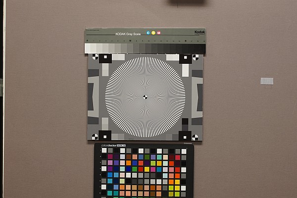
For different observers to obtain the same result the chart design and contrast should be standardized.To that end we recommend a sinusoidal Siemens star chart similar to the chart specified in ISO 12233:2014/2017, Annex E. Contrast should be as close as possible to 50:1 (the minimum specified in the standard; close to the maximum achievable with matte media). Higher contrast can make the star image difficult to linearize. Lower contrast is acceptable, but should be reported with the results. The chart should have 144 cycles for high resolution systems, but 72 cycles is sufficient for low resolution systems. The center marker (quadrant pattern), used to center the image for analysis, should be 1/20 of the star diameter.
 Acquire a well-exposed image of the Siemens star in even, glare-free light. Exposures should be reasonably consistent when multiple cameras are tested. The mean pixel level of the linearized image inside the star should be in the range of 0.16 to 0.36. (The optimum has yet to be determined.)
The center of the star should be located as close as possible to the center of the image to minimize measurement errors caused by optical distortion (if present).
The size of the star in the image should be set so the maximum spatial frequency, corresponding to the minimum radius rmin, is larger than the Nyquist frequency fNyq, and, if possible, no larger than 1.3 fNyq, so sufficient lower frequencies are available for the channel capacity calculation. This means that a 144-cycle star with a 1/20 inner marker should have a diameter of 1400-1750 pixels and a 72-cycle star should have a diameter of 700-875 pixels. For high-quality inkjet printers, the physical diameter of the star should be at least 9 (preferably 12) inches (23 to 30 cm).
Other features may surround the chart, but the average background should be close to neutral gray (18% reflectance) to ensure a good exposure (it is OK to apply exposure compensation if needed). The figure on the right shows a typical star image in a 24-megapixel (4000×6000 pixel) camera.
Run the Star module, either in Rescharts (interactive; recommended for getting started) or as a fixed, batch-capable module (Star button on the left of the Imatest main window).
In the Star chart settings window, make sure the Calculate information capacity checkbox (near the bottom of the Settings section) is checked. The SNRI settings will be described later. If other settings are correct, press OK.
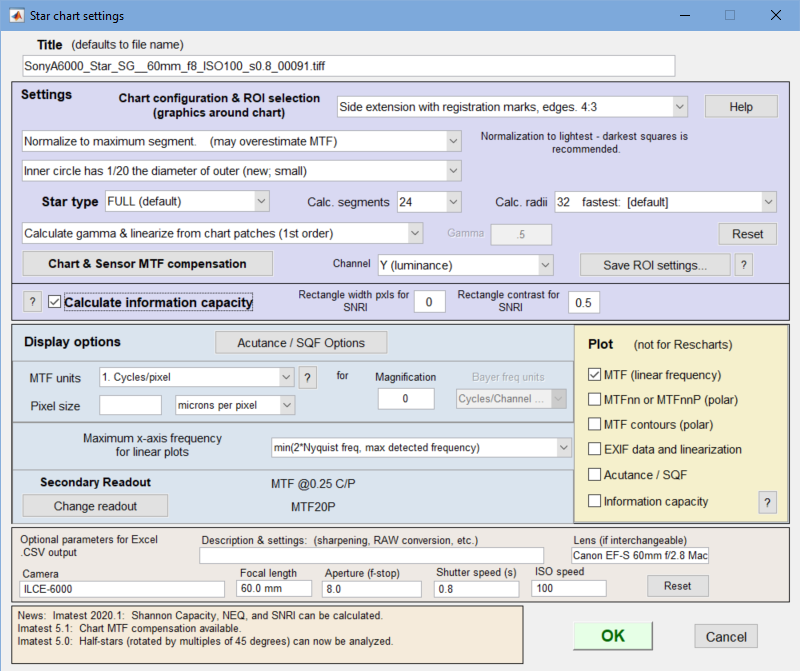
Star settings window
When OK is pressed the image will be analyzed. Any of several displays can be selected in Rescharts. The table below shows displays that are only available for information capacity measurements.
| Main display | Secondary display | Description |
| 9. Information capacity, SNRI | SNR (ratio) | Signal-to-Noise Ratio (S/N) as a function of spatial frequency for the mean segment and up to 8 individual segments |
| SNR (dB) | SNR (dB) as a function of frequency for the mean segment, etc. | |
| Signal, Noise | Signal, noise, and (S+N)/N (dB) as a function of frequency for the mean segment. | |
| Signal, 10X Noise | Signal, 10X noise, and (S+N)/N (dB) as a function of frequency for the mean segment. Useful for visualizing low levels of noise | |
| NEQ | Noise Equivalent Quanta as a function of frequency | |
| 10. Difference image (noise-only, etc.) | Noise-only (input-noiseless) | Display noise-only (with signal removed). This is a remarkable result — possibly the first time that noise has been measured and visualized in the presence of a signal. |
| Loss (input-ideal) | Input − Lossless (test chart image). Shows data that has been attenuated. Difficult to interpret. | |
| Input image | Input image (unmodified) | |
| Noiseless image | Ideal (noiseless) input image (with MTF loss), derived from Sideal. | |
| Ideal image (no MTF loss) | “Ideal” image with no MTF loss (represents the original test chart). | |
| Noise-only (linear) | Noise-only linearized. Typically darker than the gamma-encoded version. | |
| Input image (linear) | Input image linearized. Typically darker than the gamma-encoded version. | |
| 11. 3D Surface plot | Displays a 3D surface plot of signal as a function of angle (on the chart) and spatial frequency in Cycles/Pixel. Up to 8 chart cycles are shown (more would be cluttered and difficult to interpret. The image can be rotated. Note that the rectangular (angle × frequency) display area is actually pie-shaped in the chart. A small plot of signal and noise versus frequency and a summary of results is also shown. |
|
Two Rescharts displays are specifically designed for information capacity results: 9. Information capacity, SNRI, and 10. Input-noiseless Diff, etc. Here is a result from Star run in Rescharts for a raw image (converted to TIFF with dcraw using the 24-bit sRGB preset; gamma ≅ 2.2) for a high quality 24-megapixel Micro Four-Thirds camera.
Information capacity plot
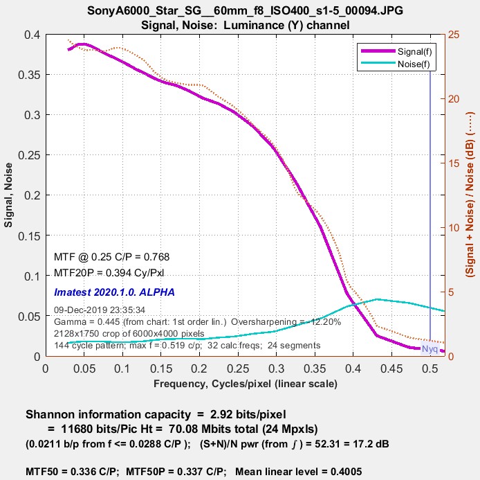
The plot below shows signal, noise, and (Signal+Noise)/Noise (db) for the 24-megapixel Micro Four-Thirds Sony A6000, set at ISO 400.
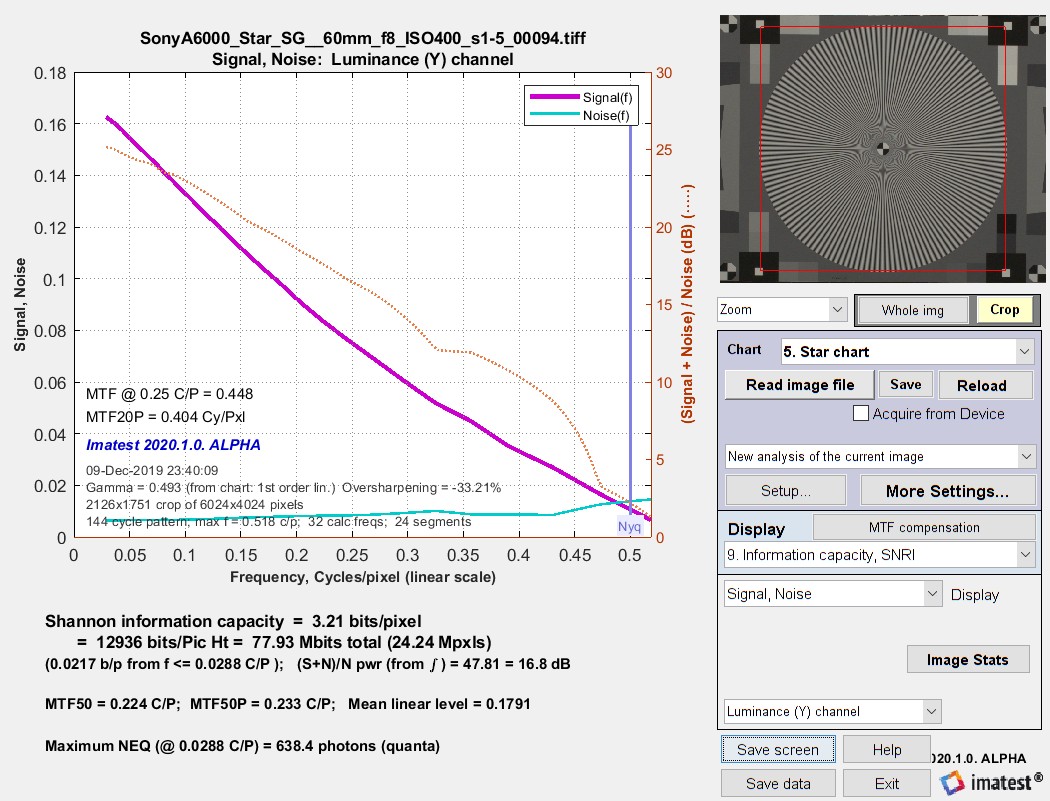
Signal, Noise, and Shannon information capacity (3.21 bits/pixel) from a
raw image (converted to TIFF) from a high-quality 24-megapixel Micro Four-Thirds camera @ ISO 400.
|
This shows results for an in-camera JPEG the same image capture. The curve has a “bump” that is characteristic of sharpening. Note that the Shannon information capacity is lower than the raw image, even though the JPEG is sharpened. This is happening because the high frequency noise is boosted, along with the signal.
Signal, Noise, and Shannon information capacity |
 |
Difference image plot (Input-noiseless, etc.)
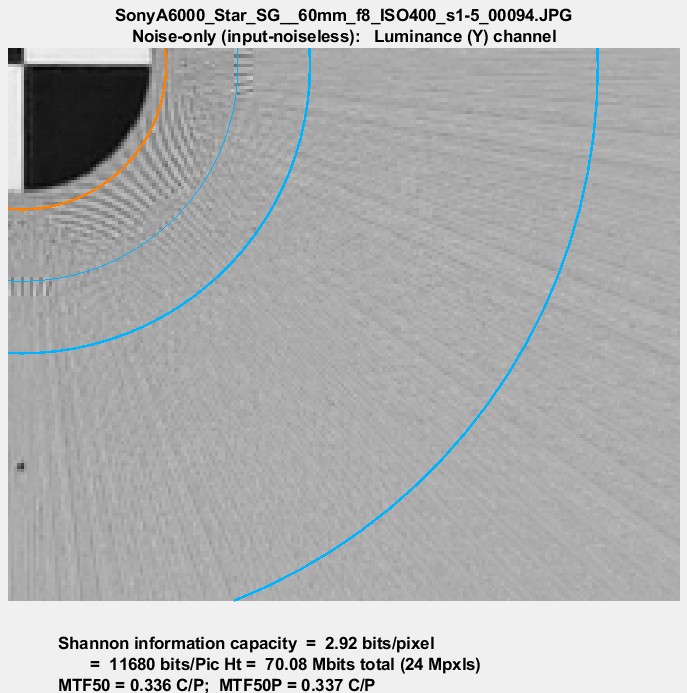
The noise-only (input-noiseless difference) plot is of particular interest because images that allow measurement and visualization of noise measured in the presence of a signal (with the sinusoldal star pattern removed) have not been previously available. Because noise is very low, and hence hard to see, at ISO 400, we illustrate noise at ISO 25600 (the maximum for the Micro Four-Thirds camera) for both TIFF from raw and JPEG images. The Copy image button on the right copies the image to the clipboard, where it can be pasted into an image editor/viewer or the Image Statistics module for further analysis.
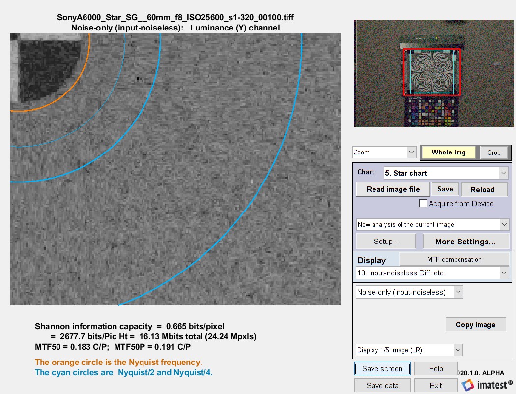 Noiseless image for Micro Four-Thirds camera, raw/TIFF image, ISO 25600.
|
The image on the right is an in-camera JPEG from the same capture at the above image (ISO 25600). It looks very different from the raw/TIFF image because noise reduction is present. The images below are for raw/TIFF and in-camera JPEG images from the same camera acquired at ISO 400. |
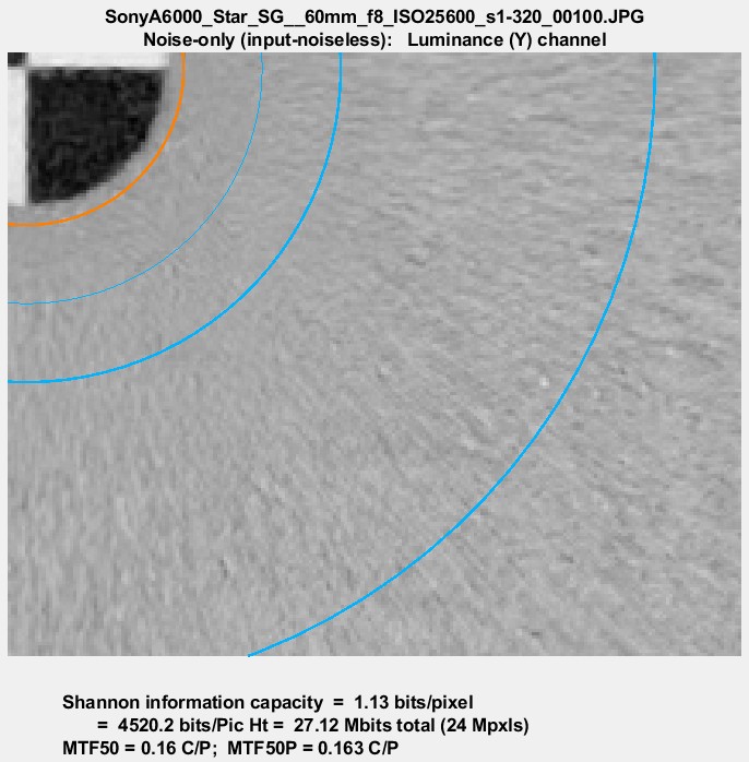 in-camera JPEG, ISO 25600 |
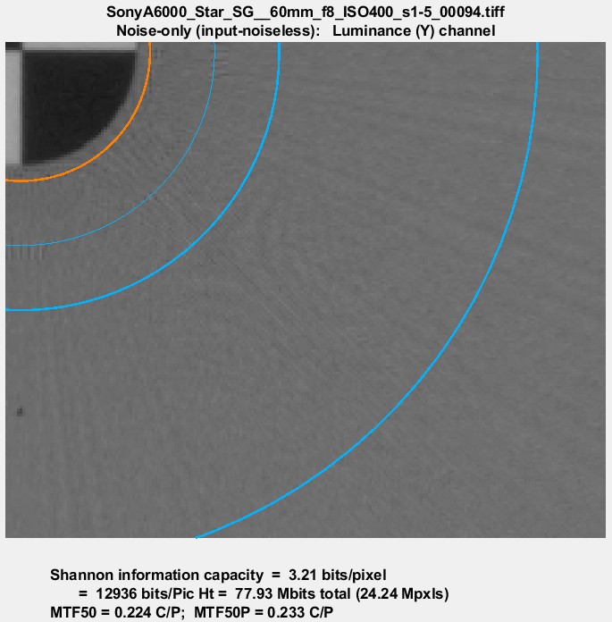 raw/TIFF ISO 400 |
 in-camera JPEG, ISO 400 |
3D Surface plot
The 3D surface plot allows you to examine small portions of the image in detail.
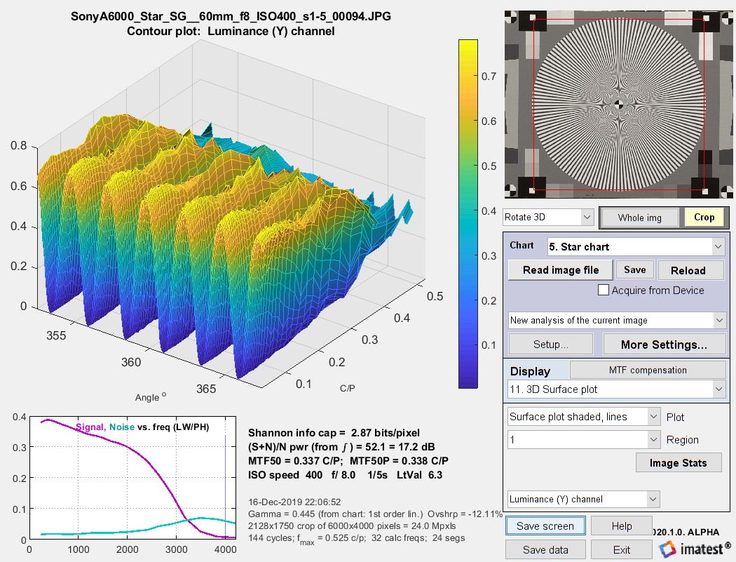 3D Surface plot for the high-quality 24 Megapixel Micro Four-Thirds camera analyzed above.
To obtain this display, 3D Surface plot calculation (as well as Calculate information capacity) must be set in the settings window. It shows the signal (for the selected channel) as a function of angle and spatial frequency (in Cycles/Pixel), which is inversely proportional to radius. This plot represents a narrow pie-slice of the original image, with angular detail at high spatial frequencies greatly enlarged.
|
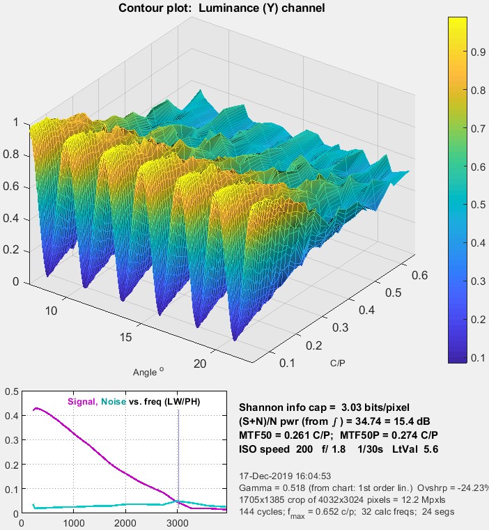
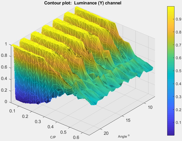
A small plot of MTF and noise as a function of spatial frequency is displayed as well as a summary of key results (information capacity, etc.). This plot was motivated by tests on an iPhone 10, where the image appeared to be saturating at low to middle spatial frequencies, but the degree of saturation was difficult to assess by viewing the image. As we can see on the right, saturation is very strong, apparently as a result of some kind of local tone mapping. It is not evident in MTF curves from the star pattern or from the adjacent slanted edges. The iPhone had some Adobe software installed that allowed both raw (DNG) and JPEG software to be captured. We don’t know if this affected the JPEG processing. The image below shows the response of a TIFF file (converted from a DNG raw image from the same iPhone 10). The response is sinusoidal— well-behaved with no amplitude visible distortion. The information capacity is nearly identical to the distorted JPEG image, where several things are happening: random noise is zero where the image is saturated, but noise as defined by \(N(\phi) = S(\phi)-S_{ideal}(\phi)\) (below), is increased by the amplitude distortion (deviation from the sine function). The insensitivity of information capacity to image processing, observed in other cases, is a remarkable result. By comparison, MTF50 and MTF50P is very much higher in the highly-processed JPEG image.
|
|

Green is for geeks. Do you get excited by a good equation? Were you passionate about your college math classes? Then you’re probably a math geek— a member of a misunderstood but highly elite fellowship. The text in green is for you. If you’re normal or mathematically challenged, you may skip these sections. You’ll never know what you missed.
Calculating Shannon capacity with Siemens star images
The pixel levels of most interchangeable images (typically encoded in color spaces such as sRGB or Adobe RGB) are gamma-encoded. For these files, pixel level ≅ (sensor illumination)1/gamma, where gamma (typically around 2.2) is the the intended viewing gamma for the color space (display brightness = (pixel level)gamma). To analyze these files they must be linearized by raising the pixel level to the gamma power. RAW files usually don’t need to be linearized (if they were demosaiced without gamma-encoding, i.e., gamma = 1).
The image of the ntotal cycle Siemens star is divided into nr = 32 or 64 radial segments and ns =8 (recommended), 16, or 24 angular segments. Each segment has a period (angular length in radians) P = 2πntotal/ns and contains nk =ntotal / nscycles and kn signal points, each at a known angular location φ, in the range {0, P}.
We assume that the ideal signal in the segment has the form
\(\displaystyle S_{ideal}(\phi) = \sum_{j=1}^{2} a_j \cos \bigl(\frac{2 \pi j n_k \phi}{P} \bigr) + b_j \sin \bigl(\frac{2 \pi j n_k \phi}{P} \bigr) \)
a and b are calculated using the Fourier series coefficient equations, derived from the Wikipedia Fourier Series page, Equation 1.
\(\displaystyle a_j = \frac{2}{P}\int_P S(\phi) \cos \bigl(\frac{2 \pi j n_k \phi}{P} \bigr) d\phi;\quad b_j = \frac{2}{P}\int_P S(\phi) \sin \bigl(\frac{2 \pi j n_k \phi}{P} \bigr) d\phi\)
where S(φ) is the measured signal (actually, signal + noise) in the segment. [Note that although this equation is not in the ISO 12233:2017 standard, it fully satisfies the intent of Appendix F, Step 5 (“A sine curve with the expected frequency is fitted into the measured values by minimizing the square error.”)]
Noise is \(\displaystyle N(\phi) = S(\phi)-S_{ideal}(\phi)\)
The frequency f in Cycles/Pixel of a segment centered at radius r (in pixels) is \(\displaystyle f = \frac{n_{total}}{2 \pi r}\). An interesting consequence of this equation is that it’s easy to locate the Nyquist frequency (0.5 C/P): \(\displaystyle r = \frac{n_{total}}{\pi}\) = 45.8 pixels for ntotal = 144 cycles.
A small adjustment (not described here) is made in case f is slightly different from the expected value due to centering errors, optical distortion, or other factors.
Signal power is \(\displaystyle P(f) = \sigma^2(S_{ideal}(f))\). Noise power is \(\displaystyle N(f) = \sigma^2(N)\), where σ2 is variance (the square of standard deviation). Note that signal + noise power is \(\displaystyle P(f)+N(f) = \sigma^2(S)\). [Note: From the context of Shannon: “Communication in the presence of noise”, we assume that N(f) is the noise measured in the presence of signal Sideal(f); not narrow-band noise of frequency f.]
The full one-dimensional equation for Shannon capacity was presented in Shannon’s second paper in information theory, “Communication in the Presence of Noise,” Proc. IRE, vol. 37, pp. 10-21, Jan. 1949, Eq. (32). This equation cannot be used directly because the pixels under consideration are two-dimensional.
\(\displaystyle C = \int_0^W \log_2 \left( 1 + \frac{S(f)}{N(f)} \right) df = \int_0^W \log_2 \left(\frac{S(f)+N(f)}{N(f)} \right) df \) [One-dimensional; not used]
This equation has to be converted into two dimensions since pixels (here) have units of area. (They have units of distance for linear measurements like MTF.)
\(\displaystyle C = \int \int_0^W \log_2 \left(\frac{S(f_x,f_y)+N(f_x,f_y)}{N(f_x,f_y)} \right) df_x\: df_y \)
where fx and fy are frequencies in the x and y-directions, respectively. In order to evaluate this integral, we translate x and y into polar coordinates, r and θ.
\(\displaystyle C = \int_0^{2 \pi} \int_0^W \log_2 \left(\frac{S(f_r,f_θ)+N(f_r,f_θ)}{N(f_r,f_θ)} \right) f_r \: df_r\: df_θ \)
Since S and N are only weakly dependent on θ, we can rewrite this equation in one-dimension.
\(\displaystyle C = 2 \pi \int_0^W \log_2 \left(\frac{S(f)+N(f)}{N(f)} \right) f \: df \)
Very geeky: The limiting case for Shannon capacity. Suppose you have an 8-bit pixel. This corresponds to 256 levels (0-255). If you consider the distance of 1 between levels to be the “noise”, then the S/N part of the Shannon equation is log2(1+2562) ≅ 16. The maximum bandwidth where information can be transmitted correctly W— the Nyquist frequency— is 0.5 cycles per pixel. (All signal energy above Nyquist is garbage— disinformation, so to speak.) So C = W log2(1+(S/N)2) = 8 bits per pixel, which is where we started. Sometimes it’s comforting to travel in circles.
Summary
- Shannon information capacity C has long been used as a measure of the goodness of electronic communication channels. It specifies the maximum rate at which data can be transmitted without error if an appropriate code is used (it took years to find codes that approached the Shannon capacity). Coding is not an issue with imaging.
- C is ordinarily measured in bits per pixel. The total capacity is \( C_{total} = C \times \text{number of pixels}\).
- The channel must be linearized before C is calculated, i.e., an appropriate gamma correction (signal = pixel levelgamma, where gamma ~= 2) must be applied to obtain correct values of S and N. The value of gamma (close to 2) is determined from runs of any of the Imatest modules that analyze grayscale step charts: Stepchart, Colorcheck., Multicharts, Multitest, SFRplus, or eSFR ISO.
- We hypothesize that C can be used as a figure of merit for evaluating camera quality, especially for machine vision and Artificial Intelligence cameras. (It doesn’t directly translate to consumer camera appearance because they have to be carefully tuned to reach their potential, i.e., to make pleasing images). It provides a fair basis for comparing cameras, especially when used with images converted from raw with minimal processing.
- Imatest calculates the Shannon capacity C for the Y (luminance; 0.212*R + 0.716*G + 0.072*B) channel of digital images, which approximates the eye’s sensitivity. It also calculates C for the individual R, G, and B channels as well as the Cb and Cr chroma channels (from YCbCr).
- Shannon capacity has not been used to characterize photographic images because it was difficult to calculate and interpret. But now it can be calculated easily, its relationship to photographic image quality is open for study.
- We stress that C is still an experimental metric for image quality. We will be happy to work with companies or academic institutions who can verify its suitability for Artificial Intelligence systems.
Information capacity from slanted-edges
|
Note: Because the slanted-edge information capacity measurement used prior to Imatest 2020.1 is inaccurate (correlating poorly with the superior Siemens star measurements) is has been deprecated completely. It has been replaced with a better measurement that is, however, only recommended for use with a Siemens star in the center of the image for calculating the total image information capacity (in units of bits/image). |
While slanted-edges are not recommended as a primary measurement of information capacity, they are potentially useful for measuring the total information capacity of the image in images where a Siemens star is located at the center surrounded by a number of stars.
History
R. Shaw, “The Application of Fourier Techniques and Information Theory to the Assessment of Photographic Image Quality,” Photographic Science and Engineering, Vol. 6, No. 5, Sept.-Oct. 1962, pp.281-286. Reprinted in “Selected Readings in Image Evaluation,” edited by Rodney Shaw, SPSE (now SPIE), 1976.
Links
The University of Texas Laboratory for Image & Video Engineering is doing some interesting work on image and video quality assessment. They approach the problem using information theory, natural scene statistics, wavelets, etc. Challenging material!
Wikipedia – Shannon Hartley theorem has a frequency dependent form of Shannon’s equation that is applied to the Imatest sine pattern Shannon information capacity calculation. It is modified to a 2D equation, transformed into polar coordinates, then expressed in one dimension to account for the area (not linear) nature of pixels.
\(\displaystyle C=\int_0^B \log_2 \left( 1 + \frac{S(f)}{N(f)} \right) df\)