Postprocessor for SFRplus, Checkerboard, and eSFR ISO for analyzing
image quality factors that require multiple images:
Curvature of field, Longitudinal (Axial) Chromatic Aberration, & more
Introduction to FocusField
FocusField is a postprocessor for displaying camera test results from batches of images acquired at different distances and/or with different focus settings (also with different apertures), then analyzed by SFRplus, Checkerboard, or eSFR ISO batch runs. (These modules are preferred because magnification, and hence distance, can be derived from the image.) It can display
- Depth of Field (DoF),
- Curvature of field,
- Longitudinal (axial) chromatic aberration, and
- Lens focal length (when used with the motorized modular test stand, which can be set for precisely-controlled distance steps).
- A comparison of results to determine the compatibility of two images intended for use in a stereo (3D) pair.
| Postprocessor comparison Each lets you compare sharpness of different regions and/or images |
|
| Postprocessor to SFR and other slanted-edge modules. Input is two CSV results files for individual regions. Lets you compare individual edges from any region of any two images (or the same image). Displays MTF for both images and transfer function (A/B) or (B/A). | |
Image Stabilization/ Sharpness Compare |
Postprocessor to SFRplus-only. Input is two or three JSON results files. Image Stabilization must be checked in the SFRplus settings window. The region selection must be the same for all the files, but files may have different sizes. Lets you compare sharpness of regions (in approximately the same location) or of the image as a while. Can compare sharpness of two image files or calculate the effectiveness of (Optical) Image Stabilization using three image files. |
| Postprocessor to SFR, Checkerboard, SFRplus, and eSFR ISO (primarily the latter three) that lets you compare summary results for several files run as a batch and stored in a file whose name has the form root file_sfrbatch.csv. Most useful for measuring sharpness at the center, part-way, corners, and weighted mean for a range of apertures, but very versatile: it can analyze any image sequence. | |
| Postprocessor for eSFR ISO, Checkerboard, and SFRplus (auto-detect slanted-edge modules that calculate magnification) that lets you calculate measurement results from batches images acquired at different distances or with different focus settings. For measuring depth of field (DoF), curvature of field, and longitudinal (axial) chromatic aberration (which varies with distance, rather than radius, for the familiar lateral chromatic aberration). Lens Focal Length (FL) can be calculated precisely when the distance increment (from the motorized modular test stand) is known. Results for batches of several files are stored in a file whose name has the form root file_sfrbatch.json. | |
Introduction – Examples – Prepare the test – Range and Increment – Acquire the images – Analyze – Run FocusField
FocusField Settings – Results – Curvature of Field – Depth of Field – Longitudinal (Axial) CA – Lens focal length
Stereo (3D) images
Examples
FocusField has two common use cases.
Vary the distance (fixed focus)
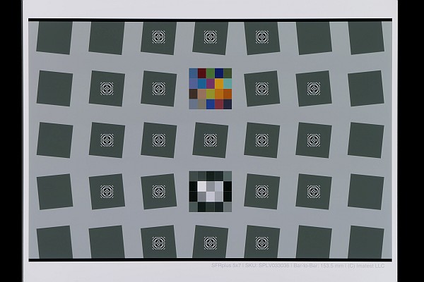
Test a camera over a range of distances with constant focus (autofocus turned off). Best focus should be close to the center of the distance range. The SFRplus, Checkerboard, or eSFR ISO charts are recommended because they contain geometric information used to calculate Magnification (and lens focal length). FocusField can test for
- Depth of Field
- exact lens focal length (magnification-based)
- Curvature of Field
- Longitudinal (axial) Chromatic Aberration
Here is an example of animated results for MTF50P (the spatial frequency where MTF falls to half its peak value) measured over a range of distances (173.5 to 162.8cm shown in the animation), obtained by pressing the Cycle button, which displays Stop below). MTF50P is a generally more stable measurement than MTF50, which can vary unpredictably in the presence of strong sharpening, as illustrated in in Sharpening. Note that the shape of the MTF50 curve on the image plane is very different in front of and behind the position of best focus. This is caused by curvature of field.
 FocusField results, cycling through distances
Vary the aperture (fixed distance)
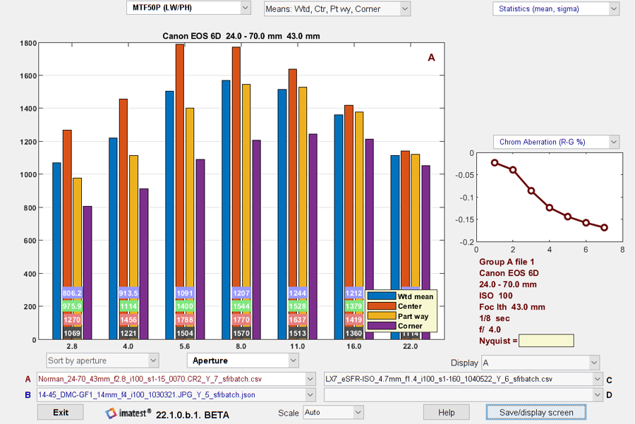
This is a common test for evaluating lens performance — especially for interchangeable lenses in DSLR and mirrorless cameras. Here is an example showing MTF50P of a DSLR camera tested at multiple apertures (f-numbers). The same lens (the first generation Canon 24-70mm L) is analyzed on www.opticallimits.com/canon_eos_ff/528-canon2470f28ff. The absolute numbers in this analysis are different because of different image processing.
 FocusField results, cycling through apertures (f-numbers)
|
A Batchview analysis of this lens is shown on the right (click to enlarge). The Weighted mean MTF for all regions as well as the mean MTF in the center, part-way, and corner regions are shown for each aperture. This result is familiar and informative, but it doesn’t catch a defect in the individual lens a first generation Canon 24-70mm f/2.8L, purchased around 2000)— a soft region on the far right, which is clearly apparent at the larger apertures (smaller f-numbers: f/2.8-f/8) in the animated Focus Field results (above). This defect is visible in landscape images. The lens traveled quite a lot in its first decade, and may have been bumped. Hard to say. It’s a monster— very heavy. These days I use much lighter equipment. |
 |
Prepare the test
Select the test chart
We recommend the SFRplus, Checkerboard, or eSFR ISO charts because they contain geometric information used to calculate Magnification, from which distance or focal length can be derived. SFRplus and Checkerboard are preferred because they have more ROIs than eSFR ISO, and hence are likely to provide more consistent results if the Field of View (FoV) changes enough to push some ROIs off the frame. These charts come in a wide variety of media: inkjet (up to 44 inches high), photographic paper (finer but smaller), B&W photographic file (12×20 inches), color film (8×10 inches), and ultra-fine Chrome on Glass (up to 4×4 inches).
 Choose the size (i.e., linear Field of View) that best matches your needs. Our charts department can help with the choice. There is an abundance (perhaps overabundance) of material on charts in the sharpness section of the Imatest documentation. Both reflective and transmissive charts work well for this application.
Framing — The chart should be framed well at the middle distance, according to the instructions for the module. For SFRplus, there should be sufficient white space above the top bar and below the bottom bar so some white space remains at the closest distance. Framing is much less critical with Checkerboard. It’s also not critical for eSFR ISO because the registration marks used for feature detection are well inside the image, but we don’t recommend eSFR ISO because it has fewer than optimum ROIs. (As we’ll see below, we recommend selecting more ROIs than are ordinarily used for standard MTF tests).
Determine the distance range and increment
Getting the distance increment right is important because if it’s too small you’ll be slowed down by having to process more data than you need, and if it’s too large you might miss important observations. Finding the right increment requires a bit of math.
When a lens is perfectly focused, a point in the object is mapped to a point in the image (neglecting diffraction and aberrations, which are always present). When the lens is not in focus, the point on the object is mapped to a circle on the image plane, called the circle of confusion or blur circle, which we prefer. The equation for the diameter of the circle is given in Wikipedia.
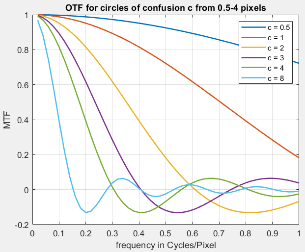
OTF in C/P for several circle of confusion diameters (c). Note that MTF = |OTF|.
For the lens is focused at S1, where the lens-to-object distance is S2,
\(\displaystyle c = \frac{S_2-S_1}{S_2} \frac{f^2}{N(S_1-f)}\)
where N is the f-number = f/A for focal length f and aperture diameter A.
The effects of the blur circle are described in Diffraction, Optimum Aperture, and Defocus, and shown in the OTF curve on the right (note that MTF = |OTF|), where the blur circle has units of pixels (i.e., the sensor pixel pitch, Dsensor). In interpreting this curve, note that the Nyquist frequency fNyq (the maximum frequency where digital data can be correctly reconstructed) is 0.5 Cycles/Pixel. For most good quality lenses, the key frequencies that characterize their performance are in the range of 0.2 – 0.5 C/P. When the normalized blur circle (c/Dsensor in the figure) is 1, MTF drops to around 0.8-0.9 in this frequency range— a reasonable change. For this reason, we recommend starting with a spatial increment ΔS = S2–S1 based on the “good enough” approximations that S2 ≅ S1 when S1 >> f, and c = Dsensor.
\(\displaystyle \Delta S = \frac{D_{sensor} \ S_1 N (S_1-f)}{f^2}\)
We can always change ΔS based on experience.
Based on the figure on the right, we guess that a sufficient range of distances can be defined by a blur circle c = 10×Dsensor.
Example — In Vary the distance (above), focal length f is approximately 80mm (based on the EXIF data), aperture N = f/4.4, S1 (the lens to chart distance in the middle of the range) is approximately 168cm = 1680mm, and the sensor pixel pitch (for the Panasonic Lumix FZ2500 camera, found on a Google search) is Dsensor = 2.41μm = 0.00241mm.
\(\displaystyle \Delta S = \frac{0.00241 \times 1680 \times 4.4 \times (1680-80)}{80^2} = 4.45\text{mm}\)
This is about half the 10mm spacing we used for the example. As we shall see from the results, this spacing was coarser than optimum. 5mm would have been optimum, and a distance range of 1680±50mm would have been sufficient (though some extra margin doesn’t hurt). The surprise was that the increment is so small: only 4.45 out of 1680mm (0.00265 = 0.265% of the distance); much lower than I would have guessed. This is a great example of math outperforming gut feeling.
Capture the images
- The test chart should be mounted and illuminated — ready to photograph.
- The camera should be mounted on a rail system and should be at one of the ends of the range of travel.
- For best results we recommend the Imatest Motorized Modular Test Stand. It lets you conveniently increment or decrement the spacing in precisely-controlled steps.
- There are other smaller, inexpensive rail systems. Most are designed for the camera to be pointed perpendicular to the rail. If you point the camera in the direction of the rail, you need to be sure the image isn’t blocked.
- You should now be ready to capture the images. Capture images by (A) pressing the shutter release gently (to minimize shake), or (B) exposing the shutter remotely. Increment the position and repeat.
- Transfer the batch of images to a computer that can run Imatest.
Analyze the batch of images
The batch of images is processed in one or two steps to prepare the combined results for FocusField. We recommend optional step 1 before running your first batch. It may be omitted if you are confident you have the correct settings and if no important settings (chart geometry, pixel pitch) have been changed.
For batches where aperture (rather than distance) is varied, we recommend running the files through Rename files to include aperture in the file name.
Step 1 (for checking and making settings) — Run an image (typically the image at the central distance or at one of the extremes) with the appropriate Rescharts (interactive/setup) module: eSFR ISO SFRplus, or Checkerboard. SFRplus will be used in this example. Use comparable settings if a different chart/module is used.
When the image is run in SFRplus Setup, the SFRplus Setup window is opened.
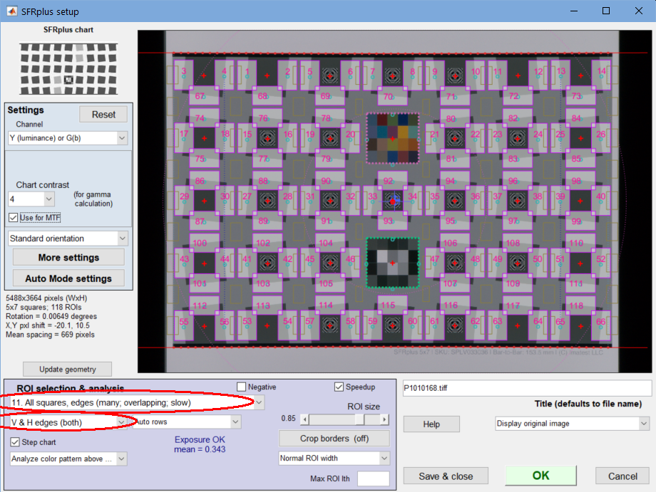 SFRplus setup window for preparing a batch run for FocusField
The key takeaway from this window is that (if possible) ALL ROIs should be selected. This is more than for normal runs. The reason is that FocusField compares sharpness at different locations in the image, and in order to accomplish this, it has to interpolate the image (to a fixed grid, currently 12 points high). Simply put, the more ROIs, the more reliable and consistent the interpolated image.
Next, press . (This can be done after pressing OK to run the image.)
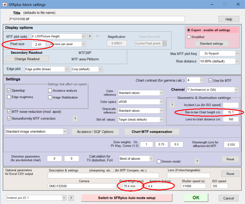
Pixel size is required for the magnification calculation.
The geometric parameter for the chart (which defines its size) must be entered for the magnification calculation.
- For SFRplus, enter Bar-to-bar chart height cm. It is distance from the top of the top bar to the bottom of the bottom bar (the distance between the outside of the bars). It should be measured carefully from the chart.
- For eSFR ISO, enter the Registration mark vertical spacing cm.
- For Checkerboard, enter the square height in cm.
Focal length (cm) and Aperture (f-number) are normally obtained from EXIF data in commercial camera files. Aperture is not critical— it’s only used for labeling. Focal length is used to calculate the distance to the chart. If the EXIF data (or Focal length) is missing, it should be entered manually in the Focal length (mm) box, as shown above.
Press to open the Auto mode window (not shown). Single region plots, which can severely slow down runs (especially when a large number of ROIs are selected, as we recommend), should be unchecked. Multi-ROI and Summary plots should checked very sparingly, if at all. In most cases they won’t be needed. Allow CSV output and Save JSON output should be checked.
Secondary readouts are important to many customers. They can be set by pressing on the upper left.
| Takeaways from Step 1: Run the Rescharts (interactive/setup) module to check/select settings: Select a large number or ROIs (preferably all). Make sure pixel size and chart geometry (bar-to-bar) are set correctly. Focal length and Aperture are also significant. Be sure Auto mode settings don’t slow down the batch run. |
Step 2 (the batch run) — Once the settings are ready, the batch run itself is straightforward.
- Run the appropriate Auto (fixed, batch-capable) module. For the recommended charts, they are , , and .
- Select the files to analyze, using the usual techniques for selecting batches.
- Click .
The output file is [root file name]_sfrbatch.json. where [root file name] is one of the files in the batch. You can view the output folder by pressing the File dropdown menu in the Imatest main window, then Open recent save folder.
Run FocusField
Press in the Imatest Classic main window to open the Focus Field window. (In the New Main window, choose “Focus Field” under the Utilities tab, in Postprocessors.)
The initial window contains brief instructions, which will be updated as the program is enhanced.
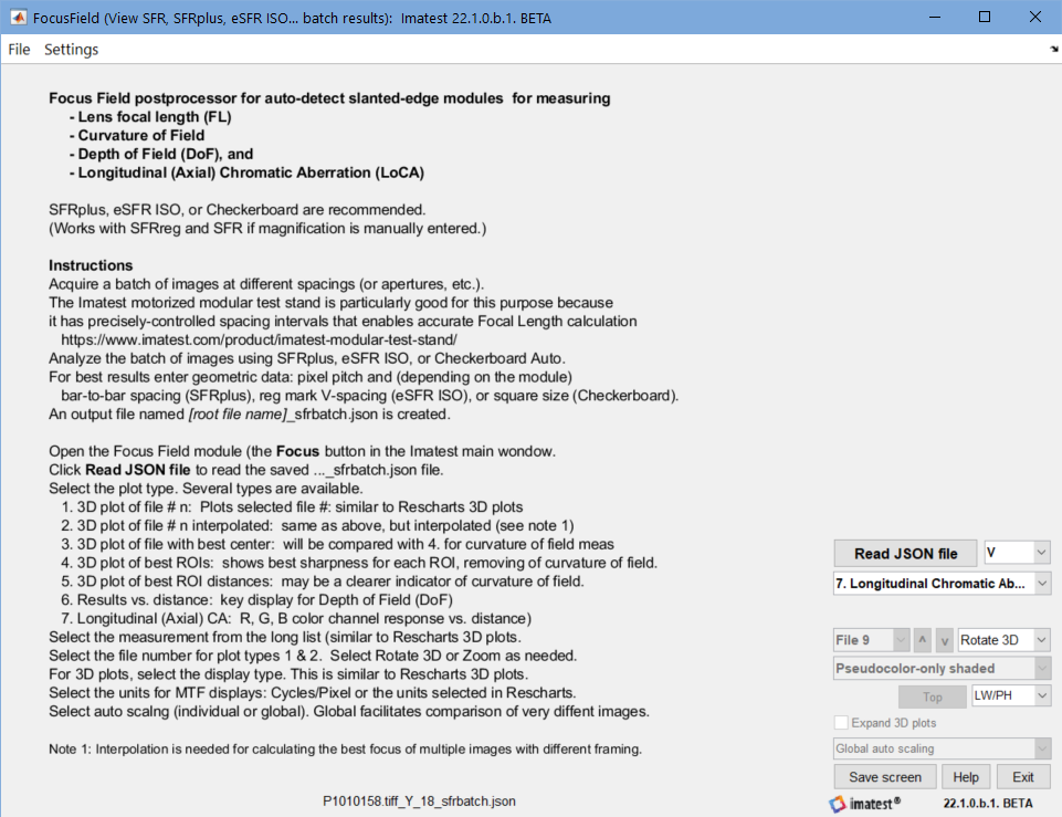 FocusField opening window, showing brief instructions
Next, press , and select the […]_sfrbatch.json file from a batch run. The contents of the screen depends on the saved settings. We begin with a plot
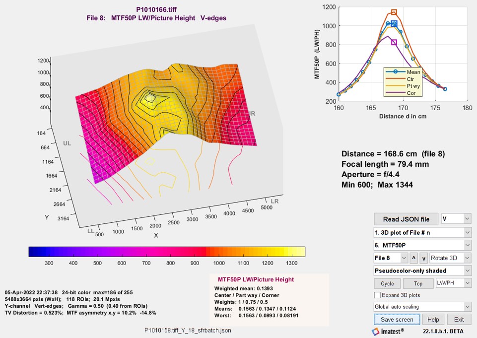 FocusField 3D plot of MTF50P (uninterpolated) + mean MTF50P vs. distance
for center, part way, and corner regions (small image on upper right)
FocusField Settings
|
|
|
| 1. | Read JSON file | Read the [name]_sfrbatch.JSON file (the output of a batch run). Required at the beginning of FocusField. |
| 2. | Edges for the 3D plot | Edges to include in calculating the 3D plot: V, H, V&H (all), Tangential (MTF), Sagittal (MTF). If
2D: Select ROIs… is selected in the Settings dropdown menu, the selected edges will be used for 2D Results plots (Plot type 6 and small plots on the upper right of Plot types 1-5). |
| 3. | Plot type |
The fundamental plot selection. Results of this setting will be illustrated below.
|
| 4. | Results to plot |
Results to plot: selected from a dropdown menu with a long list of results, derived from the Rescharts 3D plot. Note that entries 2 and 3 are Secondary readouts, which are important for many users. Although some entries may be used infrequently, we included the entire list from Rescharts. MTF50P and MTF Area Peak Normalized are our recommended sharpness metrics. Here is the complete list: {‘MTF50’; [Secondary readout 1]; [Secondary readout 2]; ‘MTF30’; ‘MTF20’; ‘MTF50P’; [‘R1090_px’]; [‘R1090_PH’]; ‘Peak MTF’; ‘LSF_PW50_pxls’; ‘CA_Area_pct’; ‘CA_Area_pxls’; ‘CA_crosssing_pct’; ‘CA_R-G_pxls’; ‘CA_B-G_pxls’; ‘Edge_roughness_pxls’; ‘Shannon_cap’; ‘Overshoot_pct’; ‘Oversharpening_pct’; ‘MTF_Area_Peak_Norml’; ‘Gamma_from_edge’; ‘Mean_ROI_level’} |
| 5. | File number | Select the file to display. Enabled for Plot types 1 and 2. and let you move up and down the list. The contents of the list can be changed in the Settings dropdown menu, which allows you to choose Select file by number (the default) or Select file by distance cm. |
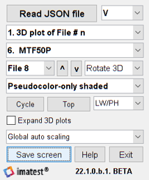
| 6. | Rotate 3D/Zoom | Lets you select 3D rotation (for 3D plots-only) or Zoom when cursor is clicked on the image. |
| 7. | 3D plot type | Lets you select the 3D plot type (one of the selections is actually 2D). A subset of the settings available in Rescharts. Settings are Pseudocolor-only, Pseudocolor-only (Shaded), and 2D image contour map. |
| 8. | Cycle | Cycle through files. Enabled for Plot types 1 and 2. This function produced the animated GIFs, above. |
| 9. | Top/Default/Recent | Viewing angle — toggles through the three settings. The default is shown above. Top view is essentially a 2D “heat map”. The Color map menu n Options II lets you select a different color scheme. |
| 10. | Units (for MTF) | Lets you choose either Cycle/Pixel (the basic calculation units of Imatest) or the selected units (LW/PH, cycles/mm, etc.) |
| 11. | Expand 3D plots | Enlarge 3D plots — helpful when regions are near the center of the image (not close to the edge). |
| 12. | Auto scaling | Auto scaling — Global is recommended when comparing different images or cycling through images. Individual provides more detail for individual images, but can be confusing when comparing different images. |
A few settings are accessible from the dropdown menu in the top bar of the FocusField window. We will add more settings from time to time.
 File dropdown
View/edit JSON file — View the JSON input file (the output of the batch run).
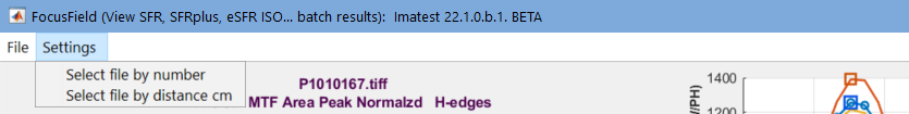
Settings dropdown
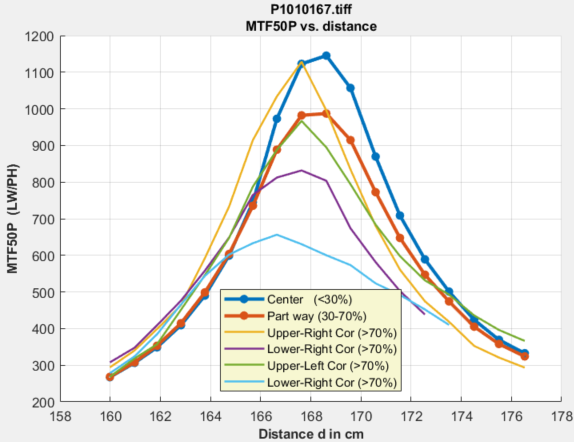
2D Results vs. distance: 2 zones, 4 corners
Select file by number — The file number appears in the Select file dropdown menu.
Select file by distance cm — The distance appears in the Select file dropdown menu.
2D Results: mean 3 zones — For Plot 6: Results vs. distance (2D) (also the thumbnail on the upper-right of plots 1-5), plot results as a function of distance for the weighted mean of all regions, and for the center (0-30%), part-way (30-~70%), and corner region (>70%). Shown in several of the figures on this page (but not the one on the right).
2D Results: 2 zones, 4 corners — For Plot 6 and the upper-right thumbnails of plots 1-5, plot results as a function of distance for the center and part-way regions and for the four corner regions (in the four quadrants: UR = Upper Right, etc.) This plot is shown on the right.
2D: All ROIs — Include ALL ROIs in the Results vs. distance plot (plot type 6 and the thumbnail on the upper right of plot types 1-5).
2D: Select ROIs (V,H,Tan,Sag…) — Include ONLY the selected ROIs (Vertical, Horizontal, both V&H, Tangential MTF, and Sagittal MTF) in the Results vs. distance plots.
Results
Curvature of Field
|
Curvature of field is one of the well-known Seidel Aberrations that causes a lens to focus on a spherical surface instead of on a plane. (Most test charts are planar.) In practice, this means that a lens that is well-focused at the center of tie image may be somewhat out of focus off-axis (at a distance from the center). Since autofocus may cause lenses to focus on off-center objects, off-axis measurements made with planar test charts may not represent the potential sharpness of the lens. Thanks to Rishi Sanyal for making a suggestion for measuring curvature of field that led to the development of the module. The key concept is that if a lens is measured multiple distances (or focus positions, which is difficult to accompligh), the best sharpness at each position for the set of distances represents the potential lens performance. To find the best sharpness at each position, we had to perform a 2-dimensional interpolation on the sharpness measurements (using MATLAB griddata). (This was required because the ROI positions were different for each image.) The lens we tested (in the Panasonic Lumix FZ2500) did not have severe curvature of field, but it had enough to measure. The 3D MTF plot of image with the best MTF at the center was not very different from the plot of the best MTF at each position. But we were able to get a meaningful plot of the best position. For vertical edges, |
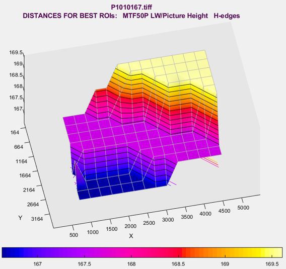 Best focus position for Horizontal edges |
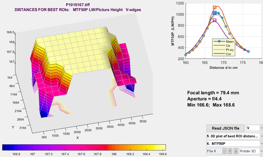
Best focus position for Vertical edges
Although it appears that curvature of field is not severe for this lens, it’s clear that the distance steps (10mm) are too coarse to resolve distance well. Half the spacing (5mm) should be sufficient for this lens — which is almost exactly what we calculated (4.45mm) in Determine the distance range and increment, above.
Depth of field (DoF)
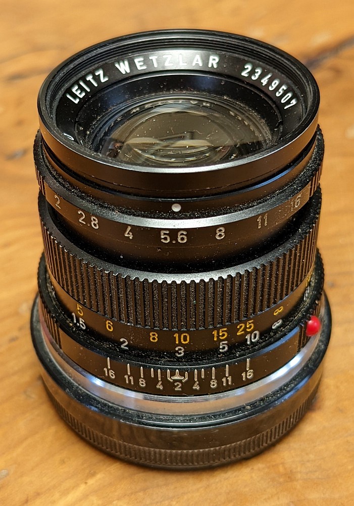
50mm Leitz (Leica) lens with DoF scale
Depth of field is the range of distances over which an image is “acceptably sharp”. The definition of “acceptably sharp” is steeped in history, and is described in Wikipedia’s Depth of Field and Circle of Confusion pages. We’ll describe the assumptions behind the common DoF definition found on most traditional cameras and lenses — with the caveat that the traditional assumptions may not be appropriate for modern machine or human vision cameras.
DoF is geometrically determined, and as such, it is not a true image quality parameter. It can be calculated for a well-characterized imaging system, but because not all systems are well-characterized, there is interest in measuring it.
An approximate equation is given in Wikipedia:
\(\displaystyle\text{DoF} \approx \frac{2 u^2 N c}{f^2}\)
for a given circle of confusion (c), focal length (f), f-number (N), and distance to subject (u).
From the Wikipedia’s confusing Circle of Confusion page, it appears that the value of c at the DoF limit on a standard-sized print (7×10 or 8×10″), designed to be viewed at 25cm, would be 0.2mm. For full-frame (24x36mm) 35mm film enlarged 7×, this translates to 0.029mm on the film plane. A commonly used rule-of-thumb is that c = d/1500, where d is the diagonal dimension of the frame.
The 50mm Summicron lens shown on the right was designed for the full-frame 35mm format. For focus set at 3 meters (≈10 feet) at f/5.6 (the marking between 4 and 8), the DoF scale indicates 8 and 12 feet (about 2.6 and 4 meters), equivalent to DoF of 1.4 meters = 1400mm. The equation gives DoF = 2 × 30002 × 5.6 × 0.029 / 502 = 1169mm.
For the 1 inch sensor in the Lumix FZ2500, the Circle of Confusion page gives the Circle of confusion diameter limit based on d/1500 = 0.011mm. Noting that the pixel size of the FZ2500 is 0.00241mm, this is 4.5 circles of confusion, which has a significant MTF loss.
For a number of reasons we do not indicate the DoF limit in FocusField output.
Longitudinal (Axial) Chromatic Aberration
Longitudinal (Axial) Chromatic Aberration (LoCA) causes different colors to focus at different points. Multiple images are required to measure it, in distinction to the more familiar Lateral Chromatic Aberration (LCA), which is caused by differences in magnification for different colors, and can be measured from a single image. LoCA is quite significant in our example, which reveals a lot about lens performance.
The thick solid Red, Green, and Blue lines with markers are the weighted means of the corresponding color channels. The lighter thin lines with markers are the centers, and the dotted lines without markers are the corners. The two strongest observations for this lens are (1) the red channel focuses closer (around 166cm) than the green and glue channels (around 168mm), and (b) the blue channel has poorer maximum MTF than the other channels.
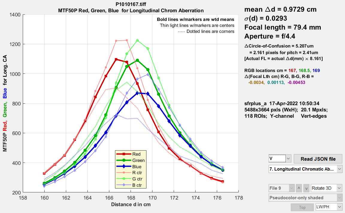 Longitudinal (Axial) Chromatic Aberration plot (color channel MTF vs. distance)
Equations — We assume that lens focal length f is different for the R, G, and B color bands (roughly centered at 610, 530, and 450 nm). Starting with the simple lens equation, \(1/f = 1/s_1+1/s_2\ \ ;\ \ \ \ f = (s_1 s_2) / (s_1 + s_2)\), where s1 is the lens to object (chart) distance and s2 is the lens-to-image (sensor) distance.
Assuming lens-to-sensor distance s2 is constant and the lens-to-object distances for two bands are d1 and d2, the change in focal lengths between different bands
\(\displaystyle \Delta f = \frac{d_1 s_2}{d_1 + s_2} – \frac{d_2 s_2}{d_2 + s_2} = s_2 \left( \frac{d_1}{d_1 + s_2} – \frac{d_2}{d_2 + s_2} \right)\)
The RGB peak MTF locations and Δf (cm) values are shown on the right of the LoCA plot. The Δf values are smaller than expected — a case where the math differs from intuitive expectations. Math generally wins.
Lens focal length
Lens focal length is normally included in the EXIF data in commercial cameras. It is usually moderately accurate (some error is expected for zoom lenses), but we have seen a case where it was incorrect (the manufacturer copied the EXIF data from an earlier model).
If the distance increment Δd between the image captures is known, as it is when the Imatest Motorized Modular Test Stand is used, focal length f can be calculated with good accuracy, based on magnification from the simple lens model. The simple lens equation for lens magnification M is
\(\displaystyle M = \frac{f}{f-d_0} \ ; \ \ \ \ \ d_0 = f(1-1/M)\)
where d0 is the lens-to-object distance, which can be measured approximately, but is difficult to measure exactly. Magnification M is derived from the geometrical measurement of the test chart (bar-to-bar height, registration mark vertical spacing, or square size for SFRplus, eSFR ISO, or Checkerboard, respectively). d0 is the distance displayed in FocusField.
Δdest, the estimated distance increment, is displayed for Plot types 6 and 7 (Results vs. distance and LoCA). It is useful when the camera is tested with the Motorized Modular Test Stand, which has a positional accuracy or around 200 microns (0.0002mm), i.e., Δd can be measured much more precisely than distance d0, and it can be used to make a very accurate estimate of lens focal length f (based on magnification M, which may be difficult to measure reliably in the presence of strong optical distortion).
If the estimated distance increment Δdest is significantly different from the known increment Δd, the estimate of focal length f can be improved over the input value (often derived form EXIF data). We start with two measurements, typically taken at the extremes of the distance range. Magnification M is different for each distance.
\(\displaystyle d_1 = f(1-1/M_1) \ ; \ \ \ \ \ d_2 = f(1-1/M_2)\)
d1 is d0 are not known exactly, but Δd = d1 – d0 is accurately known.
\(\displaystyle \Delta d = d_1 – d_2 = f(1-1/M_2) \ – f(1-1/M_1) = f(1/M_1 – 1/M_2)\)
\(\displaystyle f = \frac{\Delta d}{1/M_1 – 1/M_2} = \frac{\Delta d}{\Delta (1/M)}\)
This equation is shown in small print on the right of Plot types 6 and 7 (Results vs. distance and LoCA) as [Actual FL = actual Δd(mm) × 8.161] . For the system we analyzed, the known spacing (actual Δd) was 10mm. Therefore the actual focal length (FL) is 81.61mm— close to the 79.4mm value obtained from the EXIF data (which we never expected to be precise).
Stereo (3D) image compatibility (compare files)
This capability is different from FocusField’s other capabilities — What this feature does is display a table that allows key results for two two images to be compared conveniently.
It performs no new calculations, and we currently say nothing about the quality of the results.
It was added to Focus Field because the software infrastructure (for reading and interpreting the JSON file) was present, making it easy to code. It may be moved elsewhere in the future.
| At this time, Stereo Compare File should be regarded as preliminary — we expect to enhance it based on customer feedback. It displays a table that allows key results for two two images to be compared conveniently. |
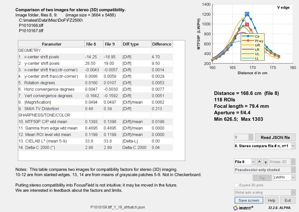 Results of comparing two images for 3D (stereo imaging) compatibility
To use this feature, run a batch of at least two images (in SFRplus or eSFR ISO auto; Checkerboard works but omits color information).
When you select File n, results of files n and n+1 are compared. In most cases, the difference (Diff type) is |Diff| = |result2 – result1| or |Diff|/mean = |result2-result1|/mean(result1,result2), where the latter is appropriate when the mean is never expected to be zero.
